Fourier-resolved energy spectra of the Narrow Line Seyfert 1 Mkn 766

Abstract

We compute Fourier-resolved X-ray spectra of the Seyfert 1 Markarian 766 to study the shape of the variable components contributing to the 0.3–10 keV energy spectrum and their time-scale dependence. The fractional variability spectra peak at 1–3 keV, as in other Seyfert 1 galaxies, consistent with either a constant contribution from a soft excess component below 1 keV and Compton reflection component above 2 keV, or variable warm absorption enhancing the variability in the 1–3 keV range. The rms spectra, which shows the shape of the variable components only, is well described by a single power law with an absorption feature around 0.7 keV, which gives it an apparent soft excess. This spectral shape can be produced by a power law varying in normalisation, affected by an approximately constant (within each orbit) warm absorber, with parameters similar to those found by Turner et al. for the warm-absorber layer covering all spectral components in their scattering scenario ($N_{H}\sim 3\times 10^{21}{\rm cm}^{-2},\log(\xi)\sim 1$). The total soft excess in the average spectrum can therefore be produced by a combination of constant warm absorption on the power law plus an additional less variable component. On shorter time-scales, the rms spectrum hardens and this evolution is well described by a change in power law slope, while the absorption parameters remain the same. The frequency dependence of the rms spectra can be interpreted as variability arising from propagating fluctuations through an extended emitting region, whose emitted spectrum is a power law that hardens towards the centre. This scenario reduces the short time-scale variability of lower energy bands making the variable spectrum harder on shorter time-scales and at the same time explains the hard lags found in these data by Markowitz et al.

1 Introduction

The X-ray emission of active galactic nuclei (AGN) is thought to be produced in the innermost regions of these systems, close to the central super massive black hole. The X-ray spectrum of most Narrow Line Seyfert 1 galaxies above 1 keV can be broadly interpreted as a power law component, probably arising from inverse Compton scattering of thermal disc photons through an optically thin corona, plus a Compton reflection component peaking towards $\sim$ 40 keV. In Narrow Line Seyfert 1s (NLS1s), a soft excess appears below $\sim 1$ keV, above an extrapolation of the power law component. This soft excess has been interpreted as either additional emission, e.g. a thermal black body or relativistically blurred ionized reflection (Fabian et al., 2002; Crummy et al., 2006) or as warm absorption on the power law component, that produces an apparent excess at energies below the absorption edges (Gierlinski & Done, 2004). Spectral fitting on its own cannot distinguish between these possibilities and indeed, gives little information on the geometry of the emitting regions. Combining spectral fitting with a study of the variability properties of the different energy bands gives information on the connection between the spectral components and their possible emission mechanisms.

The fractional variability of the X-ray light curves is energy dependent. In the case of Narrow Line Seyfert 1s, such as Mkn 766, the variability appears strongest in the middle of the XMM-Newton band, around 1–2 keV decreasing noticeably towards lower and higher energies. This behaviour suggests that the variability is produced mainly by the power law component while the soft excess and Compton reflection components remain constant (e.g Fabian et al., 2002). In this scenario, the constant components add to the flux of the variable component but not to the variability, thus diluting the fractional variability in the energy bands where they dominate the spectrum. This two-component (constant plus variable) model can broadly reproduce the flux-dependent spectral changes observed in several AGN (Taylor et al., 2003; Vaughan & Fabian, 2004) . In particular, Miller et al. (2007) have used the available $\sim 600$ ks of XMM-Newton data of Mkn 766 to show that the spectral variability of this AGN on time-scales longer than 20 ks, can be largely explained through two distinct spectral components that vary in relative normalisation.

In its simplest form, however, the two-component model cannot reproduce the time-scale dependence of the spectral variability, i.e. if only one of the spectral components varies in normalisation, the spectral changes would depend only on the relative fluxes regardless of the time-scale of their fluctuations. The fact that the energy bands behave differently on different time-scales can be readily seen through the power density spectrum (PDS), which measures the variability power as a function of Fourier frequency. In most cases, the PDS of AGN are well described by a broken power law model, with a slope of $\sim-1$ below the break and $\sim-2$ or steeper, at higher frequencies. Energy dependence of the PDS shape is normally observable around the break frequency and implies that higher energy bands are more rapidly varying. This additional variability power can appear as a flatter high-frequency PDS slope for higher energies, as in NGC 4051 (McHardy et al., 2004), as a shift of the break to higher frequencies, as observed for the first time in Mkn 766 by Markowitz et al. (2007) or as a high-frequency Lorentzian component that appears stronger in the high-energy PDS of Ark 564 (McHardy et al., 2007).

This simple two-component model can explain the energy dependence of the PDS normalisation but not energy-dependent PDS shapes. The fact that many AGN do display more short time-scale variability at higher energies does not rule out two-component models, but it implies that the variability is more complex than simple changes in normalisation of one of the components. One possibility is that the variable component changes its spectral shape when viewed on different time-scales. This can happen, for example, if softer energies are emitted by a more extended region, then their short time-scale variability can be suppressed and, therefore, the high-frequency spectrum appears harder. Alternatively, both spectral components might be variable but with different timing-properties, each one defining the behaviour of the energy bands where they dominate the spectrum.

Markowitz et al. (2007) studied in detail the energy dependence of the PDS of Mkn 766 using XMM-Newton data. They find that the 1.1–12 keV energy band has significantly more variability power than lower energy bands, on time-scales around the break in the PDS. This energy-dependent shape can be either interpreted as a shift of the break frequency to higher values for higher energies or as an additional variability component with a hard energy spectrum and a band-limited PDS. In this paper, we analyze the same XMM-Newton data set to determine the dependence of the amplitude of the variability on energy and time-scale by calculating the Fourier-resolved spectra (Revnivtsev et al., 1999). In short, this technique produces the absolute root-mean-square (rms) amplitude of variability and also the fractional rms variability (rms divided by count rate) as a function of energy and time-scale. If the variability is produced by a spectral component varying in normalisation, the Fourier-resolved spectrum will have the same shape as the variable spectral component. If there are additional constant spectral components, these will dilute the fractional variability in the energy bands where this constant component dominates. The dilution of the fractional variability is evidenced in the normalised variance spectra.

The paper is organized as follows: we describe the data reduction in Sec. 2, and the Fourier-resolved spectrum technique in Sec. 3. The resulting normalised excess variance ($\sigma^{2}_{\rm NXS}$) spectra, discussed in Sec. 4 show the characteristic shape found in other NLS1s where the $\sigma^{2}_{\rm NXS}$ peaks around 1–2 keV, at low frequencies. At high frequencies however, the $\sigma^{2}_{\rm NXS}$ spectra becomes harder. This frequency dependence is studied in more detail in Sec. 5 where we examine the spectral shape of the variable components only, through the unnormalised $\sigma_{\rm rms}$ spectra. We discuss the possible contribution of an additional spectral component to the $\sigma_{\rm rms}$ spectra in Sec. 6. In Sec. 7 we discuss the origin of the variability and frequency dependence of the $\sigma_{\rm rms}$ spectra in different possible scenarios.

2 The data

Mkn 766 was recently observed by XMM-Newton for $\sim 500$ ks from 2005-05-23 to 2005-05-31 during revolutions 999–1004 (observation ID in the range 030403[1-7]01). Here we combine this data set with earlier observations made on 2000-05-20 (obs ID 0096020101) and 2001-05-20–21 (obs ID 0109141301) during orbits 82 and 265, respectively. Spectral fitting and spectral variability analyses of these data have been published by Miller et al. (2006, 2007); Turner et al. (2007, 2006).

2.1 Observations

We used data from the EPIC PN detector (Strüder et al., 2001). In all observations, the PN camera was operated in Small Window mode, using medium filter. The data were processed using XMM-SAS v6.5.0. For each orbit, we extracted photons from a circular region of $5\arcmin$ in radius, centered on the source, and chose a background region of equal area on the same chip. Source and background events were selected by quality flag=0 and patterns=0–4, i.e. we kept only single and double events. The background level was generally low and stable, except at the beginning and end of each orbit and for $\sim 1$ ks in the middle of orbit 82 and $\sim 4$ ks in the middle of orbit 1002.

2.2 Light curves

We made light curves in 19 energy bands: 6 bands of width 0.1 keV, between 0.2 and 0.8 keV, then the following bands: 0.8–1.0, 1.0–1.3, 1.3–1.6, 1.6–2 keV, 4 bands of width 0.5 keV between 2 and 4 keV, 4 bands of width 1 keV between 4 and 8 keV, and a final band 8–10 keV. The width of the energy bands, which will define the energy resolution of the FR spectra, was chosen to keep enough counts per bin to produce reliable power spectra. The light curves were binned in 100 s bins and the background light curve were subtracted. After removing times of high background activity the final light curves had lengths of 36, 105 ,77, 96, 93, 93 and 85 ks, for orbits 82, 265, 999, 1000, 1001, 1002 and 1003 respectively. The 4 ks gap in the light curves of orbit 1002 and a 1 ks gap in orbit 82 were filled in by interpolating and adding Poisson noise deviates at the appropriate levels. We discarded the data from orbit 1004 because of its short duration as it is not long enough to cover the low frequency range used in this analysis.

Response matrices and ancillary response files were created using the XMM-SAS tasks rmfgen and arfgen, separately for orbits 82, 265 and 999-1003. The response matrices were later re-binned in energy using the task rbnrmf to match the energy bands used for the light curves.

3 Fourier-resolved spectrum technique

The Fourier-resolved spectrum (FR spectrum) technique, developed by Revnivtsev et al. (1999), calculates the root-mean-square spread, $\sigma_{\rm rms}$, of different energy bands as a function of variability time-scale. This technique was applied to AGN data for the first time by Papadakis et al. (2005), who studied the spectral variability of the NLS1s MCG–6-30-15 and later by Papadakis et al. (2007), who studied Mkn 766 (among other AGN), using the orbit 265 data only and restricted the analysis to the high energy band (3–10 keV). In all cases, the FR spectra resulted to be noticeably frequency-dependent, with higher Fourier frequencies displaying harder spectra.

The FR spectrum is calculated through the power density spectrum (PDS), which measures the variability power in different Fourier frequencies. For a discrete time series $x(t_{j})$, the normalised PDS is obtained through the discrete Fourier transform (DFT, Press et al. 1996) as:

$$P(f_{i})=\frac{2\Delta T}{N\bar{x}^{2}}|{\rm DFT}(f_{i})|^{2}=\frac{2\Delta T}{N\bar{x}^{2}}\left|\sum^{N}_{j=1}x_{j}e^{2\pi if_{i}t_{j}}\right|^{2}$$ (1)

where N is the number of points in the light curve, $\Delta T$ is the time bin size, $\bar{x}$ is the average count rate, and the Fourier frequencies are $f_{i}=i/T$, where $T$ is the length of the light curve.

The PDS, normalised by count rate, is given in terms of $\frac{\sigma^{2}}{\bar{x}^{2}}\frac{1}{\rm Hz}$, which has units of 1/Hz. When the PDS is integrated over a frequency range $\Delta f$, it produces the contribution of this frequency range to the total normalised variance $\sigma^{2}_{\rm N}$. In our case, the integration is substituted by a sum of the discrete $P(f_{i})$ for the Fourier frequencies (separated by $\delta f=1/T$), within a frequency range $\Delta f=b/T-a/T$ for integers $a$ and $b$:

$$\sigma^{2}_{{\rm N,}\Delta f}=\sum^{b}_{i=a}P(f_{i})\delta f.$$ (2)

This variance will normally be the sum of the intrinsic variability power of the source plus variability power caused by the Poisson noise associated with the counting statistics. For a continuously sampled light curve, this Poisson noise contributes a constant component to the PDS at a level of ${\rm PN_{lev}}=2(\bar{x}+B)/\bar{x}^{2}$, where $B$ is the average count rate of the background. The normalised excess variance, $\sigma^{2}_{{\rm NXS,}\Delta f}$, produced intrinsically by the source, in a given frequency range, $\Delta f$, can be computed by subtracting ${\rm PN_{lev}}$ from the $P(f_{i})$ before summing it over $\Delta f$,

$$\sigma^{2}_{{\rm NXS,}\Delta f}=\sum^{b}_{i=a}(P(f_{i})-{\rm PN_{lev}})\delta f.$$ (3)

The normalised excess variance as a function of energy, $\sigma^{2}_{{\rm NXS,}\Delta f}(E)$, is obtained simply by calculating $\sigma^{2}_{{\rm NXS,}\Delta f}$ for a series of adjacent energy bands.

The Poisson-noise subtracted rms variability, $\sigma_{{\rm rms,}\Delta f}$, is not normalised by count rate and is related to $\sigma^{2}_{{\rm NXS,}\Delta f}$ by

$$\sigma_{{\rm rms,}\Delta f}=\bar{x}\sqrt{\sigma^{2}_{{\rm NXS,}\Delta f}}$$ (4)

Calculating $\sigma_{{\rm rms,}\Delta f}$ for a set of energy bands produces the $\sigma_{{\rm rms,}\Delta f}(E)$ spectrum of the corresponding frequency range. From here on we will drop the explicit dependence on frequency range (i.e. $\Delta f$) and energy $E$, of the Fourier-resolved spectrum $\sigma_{{\rm rms,}\Delta f}(E)$ and of the normalised excess variance spectrum $\sigma^{2}_{{\rm NXS,}\Delta f}(E)$, writing simply $\sigma_{\rm rms}$ and $\sigma^{2}_{\rm NXS}$. For a given frequency range, the Fourier-resolved spectrum, $\sigma_{\rm rms}$, shows the root-mean-square amplitude of variability (in counts/s) as a function of energy, rather than the total count rate as a function of energy which composes the (time-averaged) energy spectrum.

Notice that if the amplitude of variability of each energy band is proportional to its flux (i.e. the energy spectrum, $F(E)$, only varies in normalisation but not in shape), then the $\sigma^{2}_{\rm NXS}$ spectrum will be flat, otherwise, if an energy range contains a constant component, this will appear as a dip in the $\sigma^{2}_{\rm NXS}$ spectrum. On the other hand, the $\sigma_{\rm rms}$ spectrum shows the unnormalised rms variability in each energy band, which is proportional to the count rate and fractional variability of the components of the energy spectrum and so it is unaffected by any constant spectral components. For a detailed discussion on the interpretation of the $\sigma_{\rm rms}$ spectrum, see Papadakis et al. (2007).

3.1 Calculating the Fourier-resolved spectra of Mkn 766

Vaughan & Fabian (2003) found a break in the broad-band PDS of Mkn 766 at $3\times 10^{-4}$ Hz, where the PDS slope changes from $\sim-1$ to $\sim-2$. Markowitz et al. (2007) show that the PDS is energy dependent, with more high frequency variability power at high energies. This extra power represents either an increase in the break frequency with energy or an additional band-limited variability component, peaking at $4.6\times 10^{-4}$ Hz, and with a hard energy spectrum (Markowitz et al., 2007). For the Fourier-resolved spectra, we chose three frequency bands to cover different parts of the PDS: $10^{-4.6}-10^{-4}$ Hz, $10^{-4}-10^{-3.5}$ Hz and $10^{-3.5}-10^{-3.0}$ Hz, which will be referred to as low-, medium- and high-frequency, or LF, MF and HF, ranges. The LF spectrum probes time-scales well below the break frequency, the MF probes time-scales up to this break frequency in the low energy bands and HF covers the frequency range where either the break frequency shifts with energy or where the additional variability component is located. Our aim is to determine which spectral component produces this additional high-frequency power in the high-energy bands.

For each orbit and energy band defined in Sec. 2.2, we calculated $\sigma^{2}_{\rm NXS}$ for theses three frequency ranges. Then, for each frequency range, we collected the different energy-band variances to produce $\sigma^{2}_{{\rm NXS}}(E)$ of each orbit. This dimensionless spectrum shows the variance normalised by the flux of each energy band. It is therefore sensitive to both constant and variable components of the spectrum and it is broadly independent of the energy response of the detector.

The $\sigma_{{\rm rms}}(E)$ spectra were calculated from the $\sigma^{2}_{{\rm NXS}}(E)$ spectra following Eq. 4, where the $\bar{x}$ used were the average count rates of the corresponding orbit and energy band. The raw shape of the $\sigma_{\rm rms}$ spectra depends on the response of the detector and needs to be fitted using the same response matrices as the total energy spectrum.

We averaged the $\sigma^{2}_{\rm NXS}$ spectra of orbits 999–1003 and 1000–1003, and then multiplied by the time-average energy spectra of the corresponding group of observations (i.e. 999–1003 or 1000–1003), to obtain high quality $\sigma_{\rm rms}$ spectra. As will be shown below, the variability behaviour of orbit 999 data is qualitatively different to the rest of the observations, so we will also analyse it separately. We did not combine orbit 999–1003 data with earlier observations to avoid problems with the change in energy response of the detector over the four years between the observations. The data from orbit 265 produces high quality $\sigma_{\rm rms}$ spectra on their own, owing to the high count rate of the source during that observation. We will fit the $\sigma_{\rm rms}$ spectra of orbit 265 independently, to compare with the behaviour of the combined new data. Orbit 82 produced lower quality $\sigma_{\rm rms}$ spectra due to the relatively short exposure, so we will only use this data for the comparison with single-orbit fits.

3.2 Error formulae for the frequency-resolved $\sigma^{2}_{\rm NXS}$ and $\sigma_{\rm rms}$ spectra

X-ray light curves from AGN have the variability properties of a stochastic red-noise process. This type of process produces PDS estimates distributed with a variance equal to the mean of the underlying PDS function. The error on the variance measured in a frequency range is normally estimated from the scatter of PDS estimates in the corresponding frequency bin (e.g. Papadakis & Lawrence 1993). If different energy bands are well correlated, their binned PDS estimates will also be well correlated and so the errors calculated from the spread of PDS estimates will greatly overestimate the relative errors between different energy bands, when they are observed simultaneously. This means that the noise nature of the light curves produces a large uncertainty in the amplitude of the FR spectra, but not in its shape.

For perfectly correlated energy bands, the only source of uncertainty in their relative PDS estimates is the uncorrelated Poisson noise in the light curves. Vaughan et al. (2003) calculated the error expected for $\sigma^{2}_{\rm NXS}$ of a red-noise light curve affected by Poisson noise (eq. 11 in that paper), which is appropriate for the relative scatter in variance between different energy bands. This is only a lower limit for the errors however, as the variability of different energy bands is not completely coherent. We adapted the error formulae of Vaughan et al. (2003) to produce errors for given frequency ranges, rather than for the entire power spectrum, by replacing the (unnormalised) variance due to Poisson noise, $\sigma^{2}_{\rm err}$, by the fraction of this variance contributed by a specific frequency range $\Delta f$, i.e. $\sigma^{2}_{{\rm}err,\Delta f}={\rm PN_{lev}}\times\Delta f\times\bar{x}^{2}$. The error formula for $\sigma_{\rm rms}$ uses the error on the $\sigma^{2}_{\rm NXS}$ and the conversion formula suggested by e.g. Poutanen et al. (2008). The resulting error formulae are:

$${\rm err}(\sigma^{2}_{{\rm NXS},\Delta f})=\sqrt{\left(\frac{{\rm PN_{lev}}\times\Delta f}{\sqrt{N^{\prime}}}\right)^{2}+\frac{2{\rm PN_{lev}}\times\Delta f\sigma^{2}_{{\rm NXS,}\Delta f}}{N^{\prime}}}$$

$${\rm err(\sigma_{\rm rms,}}_{\Delta f})=\sqrt{\sigma^{2}_{{\rm NXS},\Delta f}+{\rm err}(\sigma^{2}_{{\rm NXS},\Delta f})}-\sigma_{\rm{rms,}\Delta f}$$ (5)

Where $N^{\prime}$ is the number of periodogram points in $\Delta f$ and $\sigma^{2}_{{\rm NXS},\Delta f}$ is the normalised PDS integrated over $\Delta f$.

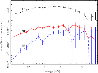
Figure 1: $\sigma^{2}_{\rm NXS}$ spectra of Mkn 766 calculated using the combined data of orbits 999–1003. The low frequency variability ($10^{-5}-10^{-4}$ Hz), in shown in dotted lines, medium frequency ($10^{-4}-10^{-3.5}$ Hz) in solid lines and high frequency ($10^{-3.5}-10^{-3}$ Hz) in dashed lines. The error bars account only for Poisson noise in the light curves and were calculated with Eq. 3.2.

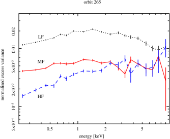
Figure 2: Same as Fig. 1 but using data from orbit 265 only.

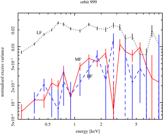
Figure 3: Same as Fig. 1 but using data from orbit 999 only. This data has the lowest count rate of all orbits and displays a much harder $\sigma^{2}_{\rm NXS}$ medium frequency spectrum.

4 Normalised excess variance spectra

The $\sigma^{2}_{\rm NXS}$ spectra of the combined 999–1003 orbit data are shown in Fig. 1 and the corresponding spectra of orbit 265 are shown in Fig. 2. In both observations, separated by 4 years, the source shows similar energy and time-scale dependencies. The low frequency component has the largest amplitude as expected, given the $1/f$ shape of the low-frequency PDS and the logarithmically broader frequency band used for LF. This low-frequency component, plotted as a dotted line, shows a smooth dip below $\sim 1$ keV and above $\sim 5$ keV, similar to the total fractional variability spectra of this and other NLS1s (Vaughan & Fabian, 2003). At high frequencies, however, the shape of the $\sigma^{2}_{\rm NXS}$ is different, as shown by the dashed line in Figs. 1 and 2. The HF normalised excess variance shows a stronger dip at low energies while the high energy dip is reduced or disappears completely, within the observational uncertainties. Note that, for each case, the LF and HF $\sigma^{2}_{\rm NXS}$ spectra have been normalised by the same time-averaged energy spectrum (i.e. total count rate per energy bin), so the difference in shape of the LF and HF spectra reveal a time-scale dependence of the variable spectral component only.

In the two-component interpretation of the main spectral variability, the energy spectra contains two fixed-shape components which vary in amplitude. If the two components vary independently, the variance spectrum can be decomposed as

$$\sigma^{2}_{{\rm NXS,\Delta}f}(E)=\frac{\sigma^{2}_{{\rm rms,\Delta}f,1}(E)+\sigma_{{\rm rms,\Delta}f,2}^{2}(E)}{(\bar{x}_{1}(E)+\bar{x}_{2}(E))^{2}}$$ (6)

where $\sigma_{\rm rms,\Delta f}(E)$ terms represent the rms spectra in a given frequency range $\Delta f$, and $\bar{x}(E)$ terms are the time-averaged energy spectra of components 1 and 2. To produce the curved shape of the variance spectra (in Figs. 1, 2 and 3), a constant, or less variable, component (1) must dominate the energy spectrum at low and high energies, therefore reducing $\sigma^{2}_{\rm NXS,\Delta f}(E)$ at those energies, while the more variable component (2) usually assumed to be a power law, might have a constant $\sigma_{\rm rms,\Delta f}(E)/\bar{x}_{1}(E)$ throughout the energy range. The observed hardening of the $\sigma^{2}_{\rm NXS,\Delta f}(E)$ spectra towards higher frequencies implies that one or both of the spectral components, $\sigma^{2}_{\rm rms,\Delta f}(E)$ get flatter at higher frequencies. This can mean that either the variable power law gets harder at higher frequencies, or that the hard part of ‘constant’ component appears constant on long time-scales but contributes significantly to the variance on shorter time-scales. To establish the energy-spectral shape of the variable components, we will fit the un-normalised $\sigma_{\rm rms}$ spectra in the following section.

The $\sigma^{2}_{\rm NXS}$ spectra of all individual orbits are qualitatively similar except for the lowest flux observation, during orbit 999, shown in Fig. 3. In this case, the MF $\sigma^{2}_{\rm NXS}$ spectrum is notably different to the LF spectrum. We will examine the variable components of this observation in detail in Sec. 6. As the data from orbit 999 appear to behave differently to all other observations, we will do the spectral fitting analysis to the combined 999–1003 and 1000–1003 data sets separately.

5 Fourier-resolved $\sigma_{\rm rms}$ spectra

Given the low resolution of the $\sigma_{\rm rms}$ spectra we will restrict the analysis to fitting simple phenomenological spectral components to obtain the broad shape of the variability components. We start by fitting the three Fourier frequency $\sigma_{\rm rms}$spectra of the combined orbits 999–1003 with a power law, affected only by Galactic absorption ($n_{\rm H}=1.7\times 10^{20}$ 1/cm²), in the 0.8–10 keV band, giving values for the power law slope of 1.93$\pm$ 0.01 for LF, 1.85 $\pm$ 0.03 for MF and 1.66 $\pm$0.04 for HF. The extrapolation of these fits to lower energies shows a ‘soft excess’ over the power law in the three Fourier-frequency spectra. A similar effect is seen in the $\sigma_{\rm rms}$ spectrum of the combined orbit 1000–1003, where the high energy power law slopes are 1.96 $\pm$ 0.01 for LF, 1.94 $\pm$ 0.02 for MF and 1.75 $\pm$ 0.04 for HF,($\chi^{2}/$dof = 3.8 for 33 degrees of freedom), as shown in Fig. 4. A similar shape was found in the FR spectrum analysis of MCG–6-30-15, presented by Papadakis et al. (2005).

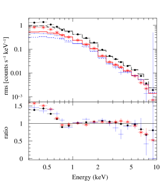
Figure 4: FR spectra of the combined 1000–1003 orbit data, LF in dashed line (black), MF in solid line (red), HF in dotted line (blue). The spectra have been fitted with a power law model at energies above 0.8 keV, and are shown extrapolated down to 0.3 keV. The power law slopes obtained are 1.96 +/- 0.01 for LF, 1.95 +/- 0.02 for MF and 1.76 +/- 0.03 for HF, ($\chi^{2}/$dof = 4.1 for 33 degrees of freedom). The three temporal-frequency spectra show an apparent ‘soft excess’.

The soft excess in the $\sigma_{\rm rms}$ spectra can be modelled as a broken power law or as a single power law with an absorption feature around 0.7 keV. We fitted the three frequency ranges with a broken power law affected by galactic absorption. The resulting fit parameters are listed in Table 1. The low and high energy slopes get flatter with increasing frequency. The low energy slope changes by approximately 0.15–0.3 and the high energy slope changes by $\sim 0.2$, unlike the case of MCG–6-30-15, where the soft power law showed no significant frequency dependence (Papadakis et al., 2005). The broken power law model generally does not produce a good fit to the $\sigma_{\rm rms}$ spectra of Mkn 766 and the residuals show systematic structure as shown in the top panel of Fig. 5.

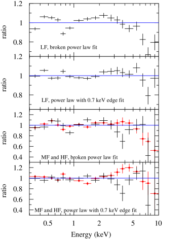
Figure 5: Ratio of the LF $\sigma_{\rm rms}$ spectrum of orbits 1000–1003, to a broken power law fit (top panel) and to a power law affected by galactic absorption and an absorption edge at $\sim$ 0.7 keV (second panel from top). The third panel shows the residuals of the broken power law fit to the MF (filled dots) and HF (crosses) $\sigma_{\rm rms}$ spectra of the same data and the bottom panel shows the MF and HF $\sigma_{\rm rms}$ spectra residuals to the warm-absorbed power law model. The power law slopes flatten with increasing frequency: for the warm-absorbed power la model the slopes are $2.14\pm 0.01$ for the LF, $2.19\pm 0.01$ for the MF and $1.95\pm 0.02$ for the HF. All fit parameters are given in Tables 1 and 2.

	$\Gamma_{L}$	$\Gamma_{H}$	break E	$\chi^{2}/$dof
999–1003
LF	2.74 $\pm$0.03	1.93$\pm$ 0.01	0.81 $\pm$ 0.02	13.5
MF	2.69 $\pm$ 0.07	1.86 $\pm$ 0.03	0.82 $\pm$ 0.04	2.90
HF	2.39 $\pm$ 0.13	1.69 $\pm$ 0.04	0.84 $\pm$ 0.1	2.64
1000–1003
LF	2.62 $\pm$0.04	1.95$\pm$ 0.01	0.77 $\pm$ 0.03	12.9
MF	2.74 $\pm$ 0.06	1.95 $\pm$ 0.02	0.79 $\pm$ 0.04	3.19
HF	2.31 $\pm$ 0.10	1.78 $\pm$ 0.04	0.86 $\pm$ 0.1	3.01
265
LF	2.79 $\pm$0.05	2.1$\pm$ 0.02	0.73 $\pm$ 0.03	6.30
MF	2.83 $\pm$ 0.08	2.07 $\pm$ 0.03	0.78 $\pm$ 0.05	2.28
HF	2.67 $\pm$0.13	1.88$\pm$ 0.03	0.76 $\pm$ 0.07	1.37

Table 1: Fit parameters, with 1$\sigma$ errors, for a broken power law with galactic absorption fit to the 0.3–10 keV FR spectra.

A better fit to the $\sigma_{\rm rms}$ spectra is obtained with a single power law affected by cold Galactic absorption and a warm absorber. Given the low resolution of the spectra presented here, we initially simply modeled the warm absorber as two edges, for O VII and O VIII, using the Xspec model zedge. The inclusion of the second absorption edge, however, does not improve the fits significantly, so we dropped one of the edge components and used a free energy for the remaining edge instead, to simulate the entire absorption feature. The best fit parameters to the combined orbits 999–1003, 1000–1003 and orbit 265 are shown in Table 2. This model produces systematically lower $\chi^{2}$ values than the broken power law model, for the same number of free parameters. The data to model ratio plots of the 1000-1003 $\sigma_{\rm rms}$ spectra fitted with this model are shown in the second (LF) and fourth (MF and HF) panels of Fig. 5. An absorption edge at 7 keV, improved the fit in both the broken power law and warm-absorbed power law cases, however, given the low resolution of the spectra and the large error bars in the high energy region, these improvements are not statistically significant.

	edge E	max $\tau$	Photon Index	$\chi^{2}/$dof
999–1003
LF	0.80 $\pm$0.01	0.71$\pm$ 0.03	2.17 $\pm$ 0.01	7.87
MF	0.80 $\pm$ 0.01	0.68 $\pm$ 0.06	2.11 $\pm$ 0.02	3.86
HF	0.85 $\pm$ 0.02	0.74 $\pm$ 0.1	1.89 $\pm$ 0.03	1.17
1000–1003
LF	0.77 $\pm$0.01	0.59$\pm$ 0.03	2.14 $\pm$ 0.01	3.40
MF	0.76 $\pm$0.01	0.62$\pm$ 0.05	2.19 $\pm$ 0.01	3.44
HF	0.85 $\pm$0.02	0.56$\pm$ 0.07	1.95 $\pm$ 0.02	0.97
265
LF	0.75 $\pm$0.01	0.55$\pm$ 0.03	2.28 $\pm$ 0.01	2.36
MF	0.76 $\pm$0.01	0.64$\pm$ 0.06	2.30 $\pm$ 0.02	1.36
HF	0.78 $\pm$0.02	0.57$\pm$ 0.08	2.09 $\pm$ 0.02	1.67

Table 2: Fit parameters, with 1 $\sigma$ errors, for a power law with galactic absorption and one edge with free energy, fit to the 0.3–10 keV FR spectra.

A third model, composed of a power law plus black body component, both affected by galactic absorption, was fitted to the $\sigma_{\rm rms}$ spectra, where the black body component was used to represent the “soft excess” feature. This model does not reproduce well the shape of the soft excess, producing residuals with structure similar to those of the broken power law model. The resulting $\chi^{2}$ values are systematically worse than for the other two models, for all orbits and frequency ranges, having values of $\chi^{2}/$dof = 28.4, 14.0 and 7.3 for the LF spectra of orbit 999–1003, 1000–1003 and 265 data sets, respectively.

The 0.3–10 keV $\sigma_{\rm rms}$ spectra are better fitted by a power law affected by cold and warm absorption, rather than two power law components joining at $\sim 0.7$ keV or a power law plus a black body component. In the power law with 0.7 keV absorption edge model fit, the spectrum hardens toward higher frequencies with a change in power law slope of $\sim 0.2$ between LF and HF, while the edge energy and optical depth remain consistent. The fact that the frequency dependence of both the low and high energy power law slopes can be explained by the flattening of a single power law provides further support to the absorbed power law interpretation.

Table 3 contains the power law with 0.7 keV absorption edge fit to the LF, MF and HF spectra of each individual orbit. The LF and MF power law slopes of each orbit are equal, while the HF slope is flatter by $\sim 0.2-0.3$ . The low flux observation, orbit 999, is an exception to this rule, in this case the power law slope changes by 0.6 between LF and MF while the HF is similar to the MF spectrum. This observation also produces the largest optical depths for the 0.7 keV absorption edge.

Orbit	Photon index	edge E	$\tau_{\rm max}$	$\chi^{2}$/dof
Low Frequency
82	2.33 $\pm$ 0.04	0.83 $\pm$ 0.02	0.90 $\pm$ 0.13	1.84
265	2.28 $\pm$0.01	0.75 $\pm$0.01	0.55 $\pm$0.03	2.36
999	2.21 $\pm$ 0.03	0.85 $\pm$0.01	1.37 $\pm$0.11	7.66
1000	2.14$\pm$0.01	0.77 $\pm$0.01	0.68 $\pm$0.03	4.03
1001	2.24$\pm$0.02	0.77 $\pm$0.02	0.41 $\pm$0.06	1.28
1002	2.15$\pm$0.01	0.78 $\pm$0.01	0.59 $\pm$0.05	3.04
1003	2.17$\pm$0.02	0.75 $\pm$0.01	0.52 $\pm$0.06	1.59
Medium Frequency
82	2.28 $\pm$0.05	0.78 $\pm$0.03	0.65 $\pm$0.16	0.67
265	2.30 $\pm$0.02	0.76 $\pm$0.01	0.64 $\pm$0.06	1.36
999	1.66 $\pm$0.07	0.87 $\pm$0.03	1.84 $\pm$0.46	1.90
1000	2.22 $\pm$0.03	0.75 $\pm$0.02	0.58 $\pm$0.09	0.48
1001	2.11 $\pm$0.03	0.79 $\pm$0.02	0.58 $\pm$0.10	1.61
1002	2.16 $\pm$0.03	0.82 $\pm$0.01	0.82 $\pm$0.10	1.77
1003	2.20 $\pm$0.02	0.72 $\pm$0.02	0.57 $\pm$0.07	1.79
High Frequency
82	1.80 $\pm$0.11	0.83 $\pm$0.06	0.89 $\pm$0.49	0.99
265	2.09 $\pm$0.02	0.78 $\pm$0.02	0.57 $\pm$.08	1.67
999	1.75 $\pm$0.1	0.84 $\pm$0.03	2.67 $\pm$0.89	1.46
1000	1.83 $\pm$0.04	0.86 $\pm$0.05	0.30 $\pm$0.14	0.84
1001	1.81 $\pm$0.05	0.84 $\pm$0.04	0.57 $\pm$0.18	1.05
1002	1.97 $\pm$0.04	0.86 $\pm$0.02	0.77 $\pm$0.13	0.74
1003	2.07 $\pm$0.04	0.82 $\pm$0.03	0.62 $\pm$0.13	0.92

Table 3: Fit parameters to the LF, MF and HF $\sigma_{\rm rms}$ spectra of the individual orbit-long observations. the model used was a power law with galactic absorption and an additional absorption edge.

6 $\sigma_{\rm rms}$ spectra of the lowest flux observation

The lowest flux observation, orbit 999, LF $\sigma_{\rm rms}$ spectrum produces the worst fit to the warm-absorbed power law model. Closer inspection of the 999 LF spectrum reveals excess rms variability around the soft excess and at the high energy end, compared to the LF spectrum of all the other orbits. Figure 6 compares the orbit 999 LF spectrum to the (rescaled) best-fitting model to orbits 1000–1003, the bottom panel shows the data to model ratio. The orbit 999 LF spectrum can be fitted by adding a black body component to the warm-absorbed power law, where the black body acts as a simple parametrisation of the soft excess. This approach produces a good fit ($\chi^{2}$/dof=17.92/14=1.28), with parameters kT=0.113$\pm$0.004 keV , Photon Index =1.55$\pm$0.03 and 0.7 keV edge parameters fixed to the best-fitting values for orbits 1000–1003. The power law slope is very flat compared to the LF rms spectra of the other observations, which have a value of Photon Index $\sim 2.2$ (see Table 3). Alternatively, it is possible that the variable component in this observation is affected by stronger warm absorption than the other orbits. To explore this possibility we used the spectral components identified in these data by Miller et al. (2007); Turner et al. (2007) using higher spectral resolution. In one of their interpretations of the spectral variability, the most variable components are a power law of slope $\Gamma=2.38$ plus an ionised reflection component whose normalisation varies tied to that of the power law, both under a warm absorber of column density $N_{H}=2.4\times 10^{21}{\rm cm}^{-2}$ and ionisation parameter $\xi=18.2$. The reflection component is modelled by the ‘reflion’ model of Ross & Fabian (2005), with solar Fe abundance and $\xi=1600$ erg cm/s. Fitting this model, allowing the normalisations and power law slope to vary, does not produce a good fit to the LF $\sigma_{\rm rms}$ spectrum of this orbit ($\chi^{2}/$dof = 7.5, for 15 dof) and requires a very flat power law of slope 1.36$\pm 0.08$. Allowing the absorbing column to vary produces a significantly better fit with $\chi^{2}/$dof = 4.2, for 14 dof with $N_{H}=6.5\pm 0.07\times 10^{21}{\rm cm}^{-2}$ and power law slope 1.77$\pm 0.09$. Fitting this model to the LF and MF $\sigma_{\rm rms}$ spectra simultaneously, with free normalisations for the power law and reflion components, produces a reasonably good fit, with $\chi^{2}/$dof = 2.89, for 30 dof. In this interpretation, the difference between the LF and MF $\sigma_{\rm rms}$ spectra in this orbit is mainly produced by a decrease in relative normalisation of the reflected component on short time-scales. The ratio of power law to reflion normalisation rises from 1.86$\times 10^{4}$ in the LF to 8.37$\times 10^{4}$ in the MF.

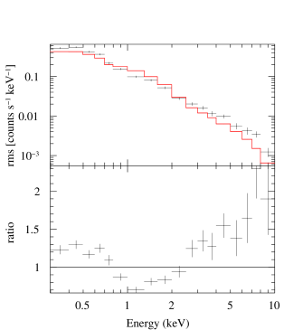
Figure 6: Top: LF $\sigma_{\rm rms}$ spectrum of the lowest flux observation, orbit 999, in black markers with error bars, the solid line represents the warm-absorbed power law model fit to the combined orbits 1000–1003 LF data and variable normalisation. The bottom panel shows the data to model ratio, showing excess rms variability in the ‘soft excess’ and high energy parts of the spectrum.

The 1–10 keV range of the energy spectrum of orbit 999 is probably not a single component, as Fig. 3 shows that the fractional variability of the LF spectrum in this range changes from being uniform to dropping sharply at around 3 keV. A natural explanation for the $\sigma_{\rm rms}$ and fractional variability spectra of orbit 999 is that the very strong soft excess and hard power law in the energy spectrum of this orbit are weakly varying, diluting part of the fractional variability at low and high energies but still contributing significantly to the total rms. In this interpretation of the $\sigma_{\rm rms}$ spectrum, orbit 999 might be essentially equal to all the other observations with the only difference that the power law component flux is weak compared to strong-flux, weakly varying additional components. If this is the case, then the difference between the LF and MF $\sigma_{\rm rms}$ spectra of orbit 999 should be due to the variability properties of these additional components only, as in all other observations the LF and MF spectra have approximately the same shape.

We fitted the LF and MF 999 $\sigma_{\rm rms}$ spectra with the best-fitting warm-absorbed power law model of orbits 1000–1003, with all parameters fixed except for the normalisation, plus a black body component, and an additional hard power law of Photon Index=1 with an absorption edge at $\sim$7 keV. These additional components are a simple parametrisation of the 0-point in the principal component analysis of (Miller et al., 2007), where the $\sim 7$ keV edge is detected significantly. We did not use a single absorbed or reflected component for the additional soft excess and hard power law since these features show different time-scale dependencies. Both absorption edges, at 0.7 and 7 keV were applied to all components. The optical depth of the 7 keV edge and the black body temperature were fitted jointly to the LF and MF spectra and the normalisations of all components were allowed to vary independently. Note however that the $\sigma_{\rm rms}$ variability of independent components should add quadratically and our fitting procedure adds components linearly. This is only a problem in energy bins where the different components have similar amplitudes, so we expect to obtain the approximate normalisation of the different components but not to reproduce the spectral shape exactly.

The top panel of Fig. 7 shows the 999 LF $\sigma_{\rm rms}$ spectrum, fitted with a black body component and hard power law in addition to the warm-absorbed power law model fitted to the other orbits, showing that it can describe the LF spectrum well. The bottom panel in this figure shows the same model components fit to the 999 MF spectrum. The combined fit to the LF and MF spectra produces a $\chi^{2}$/dof=38.8/27=1.44. Fitting the same components to the average spectrum of this orbit, allowing only the normalisations to vary, we can estimate the fractional variability of the black body component as rms/$\bar{x}=7\pm 1$% at low frequencies and $1.9\pm 1.0$% at medium frequencies, the fractional variability of the hard power law however remains constant, $7.8\pm 1.4$% fot LF and $7.9\pm 1.7$% at MF, indicating that the additional soft excess and hard power law components behave differently on different time-scales and cannot be part of a single, rigid component. The fact that this additional soft excess is more variable on long time-scales might be a product of the soft excess responding to the large amplitude continuum variations.

The orbit 999 HF $\sigma_{\rm rms}$ spectrum is similar to the corresponding MF spectrum but with much poorer signal-to-noise, given the low variability power in the high frequency band and the low count rate in this orbit, so we did not attempt a complex fit to these data.

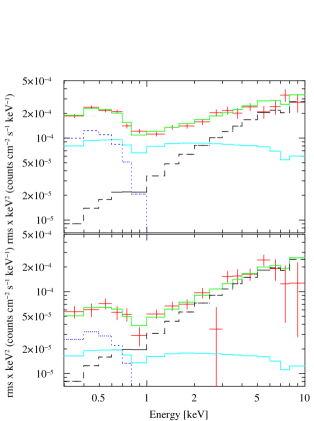
Figure 7: LF (top) and MF (bottom) unfolded $\sigma_{\rm rms}$ spectra of the lowest flux observation, orbit 999, in red markers with error bars, fitted with the best fitting absorbed power law model to orbits 1000–1003 in light blue solid line, plus a simple parametrisation additional soft excess,represented by a black body (blue dotted line) and a hard power law (black dashed line). In this interpretation, the difference in shape of the LF and MF 999 $\sigma_{\rm rms}$ spectra is explained by the relative weakening of the soft power law (as seen in the other orbits) together with a weakening of the soft excess, while the hard power law component remains equally variable in both frequency ranges.

7 discussion

We have calculated the normalised excess variance spectra, $\sigma^{2}_{\rm NXS}$, of Mkn 766, in three different time-scale ranges. The low-frequency normalised variance spectra show the characteristic shape seen in other NLS1s, where the fractional variability peaks at energies of 1–3 keV. The drop in fractional variability below 1 keV and above 3 keV can indicate the presence of less variable components, that dominate the spectrum in those energy ranges, or alternatively, varying amounts of warm absorption, enhancing the variability at energies where the opacity is largest. For the first time in AGN X-ray data analysis, we calculate the normalised excess variance spectrum for different frequency ranges, finding that this characteristic peaked shape is only produced by long time-scale fluctuations. We show that on shorter time-scales (around and above the break frequency in the PDS) the fractional variability drops strongly at low energies, while at high energies the drop becomes less pronounced or disappears completely. We then used the un-normalised $\sigma_{\rm rms}$ spectra, i.e. Fourier-resolved spectra, to study which spectral components produce this time-scale dependence in the $\sigma^{2}_{\rm NXS}$ spectra.

The most variable component in the energy spectrum of Mkn 766 appears in the $\sigma_{\rm rms}$ spectra as a power law affected by cold (Galactic) and warm absorption, which give it the appearance of a power law plus a soft excess. At frequencies around the break frequency in the PDS, the $\sigma_{\rm rms}$ spectrum hardens by 0.2 in power law slope, this behaviour is observed in two independent observations of the source, in orbit 265 and the combined 1000–1003, separated by 4 years. The fact that the hardening of both the ‘apparent soft excess’ and the power law in the $\sigma_{\rm rms}$ spectra are consistent with a change in slope of a single absorbed power law strengthens the interpretation that both features correspond to a single component. Therefore, the soft excess seen in the average energy spectrum can be composed of both, (constant) warm absorption on a power law component and an additional, less variable soft component that produces the drop in the $\sigma^{2}_{\rm NXS}$ spectrum.

This interpretation is in agreement with the scattering scenario in the time-resolved spectral analyses of Miller et al. (2007); Turner et al. (2007), where the spectral variability is mainly explained by a variable power law continuum and approximately constant scattered component. Miller et al. (2007) have used principal component analysis to show that the spectral component producing most of the flux variability (PC1) is not a simple power law but it contains an apparent soft excess, caused by the presence of a low column of absorbing gas ($N_{H}\sim 3\times 10^{21}{\rm cm}^{-2},\log(\xi)\sim 1$, with $\xi$ in units of erg cm/s), and an Fe line and edge. This absorber, which roughly corresponds to the $N_{H}(3)$ component in the scattering scenario in Turner et al. (2007), is consistent with the warm absorber on the power law in our fits to the $\sigma_{\rm rms}$ spectra. Below, we speculate on the origin of the observed flux variability and on the time-scale dependence of the $\sigma_{\rm rms}$ spectra.

7.1 Variable absorption or intrinsic continuum variability

The spectral variability in these data has been studied using principal component analysis (Miller et al., 2007) and time-resolved spectral fitting (Turner et al., 2007). These analyses show that the spectral variability is either produced by a warm absorber covering a variable fraction of the continuum power law emission, affecting mainly the flux in the 1–3 keV range, or by a warm-absorbed power law varying in normalisation in addition to a less variable component containing a soft excess and a hard power law. Both scenarios produce larger fractional variability in the 1–3 keV band which can reproduce the normalised excess variance spectra at low frequencies.

We note that the parameters of the absorbers that produce the variability in the partial covering model, found by Turner et al. (2007), can produce a maximum to minimum flux ratio of $\sim 1.5$ in the 5–10 keV band, from uncovered to totally covered continuum. The maximum to minimum flux ratio in this band in the data (using 25 ks bins) is 2.7 within orbits 999-1003 and 3.5 when all the data are included. This indicates that either the absorption is much stronger than what is currently resolved (as, for example, Compton-thick ‘bricks’ in the line of sight producing additional variability in the entire energy range) or that the main source of variability in the 5–10 keV band is largely intrinsic to the continuum flux. The variations on time-scales of $\sim 25$ ks are well correlated between different energy bands, although they are larger at medium energies. In the case where the 5–10 keV variability is mainly driven by intrinsic continuum variations, this correspondence would imply that either most of the variability in the entire energy range is produced by the same continuum variations, or that the strength of the absorption is well correlated to these variations. The latter case is possible if the changes in the absorption strength are produced by changes in the ionisation parameter, instead of covering fraction. The ionisation state can easily depend on incident flux and, as an increase in flux can lead to higher ionisation and therefore lower opacity and even higher observed luminosity, this effect can easily produce the desired effect of enhanced variability in the 1–3 keV range, where the warm-absorber opacity is highest.

If the flux variability is intrinsic to the continuum, the larger fractional variability at medium energies can be produced by constant or less variable spectral components diluting the fractional variability at the extremes of the observed energy band. In this scenario, all the timing properties can be essentially contained in the flux variability of the continuum, which can be achieved through fluctuations in the accretion rate, as explained in Sec. 7.3. In this case, an approximately constant warm ab sober covering the varying continuum can produce the $\sigma_{\rm rms}$ spectra of the observed shape. This case would correspond to the ‘scattering scenario’ for spectral variability described in e.g. Turner et al. (2007), where the fractional variability spectrum requires the presence of a less variable scattered component.

7.2 Origin of the time-scale dependence of the $\sigma_{\rm rms}$ spectra

The $\sigma_{\rm rms}$ spectra steepen by about 0.2 in power law slope between the MF and HF regimes. This steepening can be intrinsic to the varying power law continuum, if for example softer X-rays are emitted by a larger region which therefore quenches the high-frequency variability, making the HF spectrum look harder. Notice that this scenario does not produce nor imply spectral pivoting. Alternatively, approximately constant absorption can change the slope of the $\sigma_{\rm rms}$ spectra if the region producing high frequency variability is more strongly absorbed and therefore shows a harder spectrum. In either case, the primary emitting region needs to be extended and produce different time-scales of variability in different regions, as for example, variability produced by the accretion flow on radially-dependent time-scales. The first case would also require that the emitted spectrum harden toward the centre of the system, while the second requires larger columns of absorbing material and/or higher covering fractions obscuring the innermost regions, where the HF variability would be produced. The HF spectra covers timescales between 1000 and 3200s, for a black hole mass of $3.5\times 10^{6}M_{\odot}$ (Botte et al., 2005), 3000s corresponds to a light crossing time of 200 gravitational radii ($R_{g}=GM/c^{2}$) and to the orbital period at $\sim 10R_{g}$. If intrinsic to the primary continuum, the HF variability is probably produced within a region of this size, so if constant absorption is producing the change in $\sigma_{\rm rms}$ spectral slope, the additional obscuring material has to cover only a region of a few tens of $R_{g}$.

In the case where the variability is mainly driven by changes in the intrinsic continuum flux, a steepening of the $\sigma_{\rm rms}$ spectra could still be produced by some amount of variable absorption. Variable absorption increases the rms variability mostly in the energy bands where the absorption is strongest, producing $\sigma_{\rm rms}$ spectra with a shape similar to the reciprocal of the opacity as a function of energy. As mentioned above, the absorbing material parameters found for this source do not affect strongly the high energy band (5–10 keV), therefore, this process cannot enhance the high energy variability without enhancing the variability at lower energies much more. As a consequence, variable absorption can only make the $\sigma_{\rm rms}$ spectra softer. To fit the observed behaviour, this process would have to enhance the low energy variability on long time-scales, covered by the LF and MF spectra and not the short time-scale variability, therefore producing comparatively harder HF $\sigma_{\rm rms}$ spectra. Notice however, that the time-scale where variable absorption should start becoming important needs to coincide with the time-scale at which the power spectrum of the continuum variability breaks, to produce the change in slope of the $\sigma_{\rm rms}$ spectra at the correct time-scale.

Finally, it is also possible that the hardening of the $\sigma_{\rm rms}$ spectra between the LF and HF regimes is produced by a separate variable spectral component, with a hard energy spectrum and strong high-frequency variability. In this interpretation, the power law spectral component can have the same slope at all variability time-scales and the time-scale dependence we observe in the $\sigma_{\rm rms}$ spectra would be produced by the stronger variability of a hard component at frequencies of $3\times 10^{-4}-10^{-3}$ Hz. The spectrum of this additional component would then correspond to the spectrum of the possible QPO detected in the PSD of Mkn 766 at $4.6\times 10^{-4}$ Hz (Markowitz et al., 2007). The present data are insufficient to distinguish between an intrinsic hardening of the power law and the appearance of a separate variability component. We note however, that it is unlikely that this possible hard component corresponds to the reflection component. Light travel times to the reflector will smooth short time-scale variability which is inconsistent with this hard component displaying more high-frequency power than the incident continuum.

7.3 Propagating fluctuations

One interpretation of the change in slope of the $\sigma_{\rm rms}$ spectra with frequency is that fluctuations on different time-scales originate in different regions, each one emitting a power law energy spectrum with its characteristic slope. Given that, for each observation, the absorption parameters of the $\sigma_{\rm rms}$ spectra at different frequencies are similar, it is possible that all these emitting regions are covered by the same (approximately constant) absorber. This configuration is expected if the power law component is emitted by a corona close to the central black hole, with absorbing material, such as a wind, in the line of sight to the centre.

The behaviour of the $\sigma_{\rm rms}$ spectrum can be understood in the context of propagating-fluctuation models, where the emitted spectrum hardens towards the centre. Propagating-fluctuation models relate the variability to accretion rate fluctuations, that are introduced at different radii in the accretion flow with a radially-dependent characteristic time-scale, e.g. proportional to the local viscous time-scale. This scenario was introduced by Lyubarskii (1997) to explain the wide range of variability time-scales present in the X-ray light curves of accretion powered systems, and explains several other variability properties (Arévalo & Uttley, 2006). Kotov et al. (2001) have shown that if the emitted energy spectrum hardens inward, then this model produces more high-frequency power at higher energies and also time lags, where harder bands lag softer ones.

Churazov et al. (2001) note that a standard geometrically thin accretion disc cannot produce and propagate short time-scale accretion rate fluctuations due to its long characteristic time-scales. A geometrically thick accretion flow, however, can easily maintain and propagate these rapid fluctuations. In their proposed configuration, the thermally-emitting geometrically thin disc is sandwiched by a thick accretion flow, which acts as an accreting corona, responsible for the Comptonised X-ray emission seen as the power law spectral component in galactic black hole candidates and AGN. Therefore, a stable disc emission and highly variable power law emission can coexist, where the variability arises from accretion rate fluctuations in the corona. Note that in a standard accretion flow the drift velocity scales with the scale height squared, $(H/R)^{2}$, if the corona is 10 times thicker than the geometrically thin disc and its surface density is only 1 % that of the thin disc, the accretion rate of both flows are comparable. This simple argument shows that even a tenuous corona can have a significant impact on the total accretion rate and so it is not unreasonable to think that it can produce most of the observed X-ray flux variability in AGN.

This interpretation, where fluctuations propagate inwards in the accretion flow and the spectrum hardens in the same direction, produces hard lags (Kotov et al., 2001; Arévalo & Uttley, 2006), as observed in these data (Markowitz et al., 2007). In this scenario, increasingly shorter variability time-scales are produced closer to the centre, and therefore, the corresponding high-frequency $\sigma_{\rm rms}$ spectrum shows a harder energy spectrum, characteristic of its region of origin.

References

- Arévalo & Uttley (2006) Arévalo, P., Uttley, P., 2006, MNRAS, 367, 801
- Botte et al. (2005) Botte, V., Ciroi, S., Di Mille, F., Rafanelli, P., Romano, A., 2005, MNRAS, 356, 789
- Churazov et al. (2001) Churazov, E., Gilfanov, M., Revnivtsev, M., 2001, MNRAS, 321,759
- Crummy et al. (2006) Crummy, J. , Fabian, A. C., Gallo, L., Ross, R. R., 2006, MNRAS, 365, 1067
- Fabian et al. (2002) Fabian, A., Ballantyne, D. R., Merloni, A., et al., 2002, MNRAS, 331, L35
- Gierlinski & Done (2004) Gierliński, M. , Done, C., 2004, MNRAS, 349, L7
- Kotov et al. (2001) Kotov O., Churazov E., Gilfanov M., 2001, MNRAS, 327, 799
- Lyubarskii (1997) Lyubarskii Y. E., 1997, MNRAS, 292, 679
- Markowitz et al. (2007) Markowitz A., Papadakis I., Arévalo, P., et al., 2007, ApJ, 656, 116
- McHardy et al. (2004) McHardy I. M., Papadakis I. E., Uttley P., Page M. J., Mason K. O., 2004, MNRAS, 348, 783
- McHardy et al. (2007) McHardy I. M., Arévalo, P., Uttley P., et al., arXiv.0709.0262
- Miller et al. (2007) Miller L., Turner T. J., Reeves J. N., et al., 2007, A&A, 463, 131
- Miller et al. (2006) Miller L., Turner T. J., Reeves J. N., et al., 2006, A&A, 453, L13
- Papadakis et al. (2005) Papadakis I.E., Kazanas D., Akylas A., 2005, ApJ, 631, 727
- Papadakis et al. (2007) Papadakis I.E., Ioannou Z., Kazanas D., 2007, ApJ, 661,38
- Poutanen et al. (2008) Poutanen J., Zdziarski A., Ibragimov A., arXiv0802.1391
- Revnivtsev et al. (1999) Revnivtsev M., Gilfanov M., Churazov E., 1999, A&A, 347, L23
- Ross & Fabian (2005) Ross R.R, Fabian A.C., 2005, MNRAS, 358, 211
- Strüder et al. (2001) Strüder, L., Briel, U., Dennerl, K., et al. 2001 A&A, 365, L18
- Taylor et al. (2003) Taylor R., Uttley P. McHardy I. 2003, MNRAS, 342, L31
- Turner et al. (2006) Turner, T. J., Miller, L., George, I. M., Reeves, J., 2006, A&A, 445, 59
- Turner et al. (2007) Turner, T. J., Miller, L., Reeves, J. N., Kraemer, S. B., arXiv.0708.1338
- Uttley & McHardy (2001) Uttley P., McHardy I. M., 2001, MNRAS, 363, 586
- Vaughan & Fabian (2003) Vaughan S., Fabian A.C., 2003, MNRAS, 341, 496
- Vaughan et al. (2003) Vaughan S., Edelson R., Warwick R. S., Uttley P., 2003, MNRAS, 345, 1271
- Vaughan & Fabian (2004) Vaughan S., Fabian A. 2004, MNRAS, 348, 1415