A Dual Path Integral Representation for Finite Temperature Quantum Field Theory

Abstract

We impose the periodicity conditions corresponding to the Matsubara formalism for Thermal Field Theory as constraints in the imaginary time path integral. These constraints are introduced by means of time-independent auxiliary fields which, by integration of the original variables, become dynamical fields in the resulting ‘dual’ representation for the theory. This alternative representation has the appealing property of involving fields which live in one dimension less than the original ones, with a quantum partition function whose integration measure is identical to the one of its classical counterpart, albeit with a different (spatially nonlocal) action.

1 Introduction

Quantum Field Theory (QFT) models with constrained configuration spaces naturally arise within the context of modern applications, particularly gauge invariant systems [1].

More recently, a formulation involving constraints has been also applied to deal with different kinds of problems, namely, the static and dynamical Casimir effects [2, 3, 4], and to derive the overlap Dirac operator [5, 6] in a simpler way [7]. There, fields used to impose the constraints lead, after integrating out the original variables, to an effective model where the dynamical fields live on the constrained surface. Since the codimension of the boundaries is usually equal to $1$, the effective model is defined in one dimension less than the original one.

Here, we present the extension of that kind of approach to a less natural realm, that of QFT at finite temperature ($T>0$), to deal with the periodicity constraints in the imaginary time. The foundations of QFT at $T>0$ were laid down quite a long time ago [8, 9]. The original approach to this topic, the now called Matsubara (or ‘imaginary-time’) formalism has been very successful indeed in allowing for the evaluation of thermal effects in QFT, both in High Energy [10] and Condensed Matter Physics.

It allowed, for example, to study the new phenomena that emerge when using a Statistical Mechanics description for quantum relativistic systems. It also provided a convenient way to naturally extend the notion of Abelian and non Abelian gauge fields, studying its consequences for particle physics [10, 11, 12], in the $T>0$ context.

A fundamental property introduced by this formalism is the imaginary-time periodicity (antiperiodicity) conditions for the bosonic (fermionic) field configurations in the path integral. That may be clearly seen already at the level of the partition function, ${\mathcal{Z}}(\beta)$, for a system at a temperature $T=1/\beta$, with a Hamiltonian ${\widehat{H}}$:

$${\mathcal{Z}}(\beta)\;=\;{\rm Tr}\big{(}e^{-\beta{\hat{H}}}\big{)}\,.$$ (1)

Assuming first, for the sake of simplicity, that there is only one (bosonic) degree of freedom, described by a coordinate $q$, the expression above may be written more explicitly as follows:

$${\mathcal{Z}}(\beta)\;=\;\int dq\;\langle q|e^{-\beta H}|q\rangle\;=\;\int dq\;\langle q,-i\beta|q,0\rangle\;,$$ (2)

where $|q,t\rangle$ denotes the usual ‘rotating basis’ elements, which here appear evaluated at imaginary values of $t$. Then the standard path integral construction for the transition amplitude between different times may be applied, to obtain the partition function in the Matsubara formalism:

$${\mathcal{Z}}(\beta)\;=\;\int_{\rm q(0)=q(\beta)}\,{\mathcal{D}}p\,{\mathcal{D}}q\;e^{\int_{0}^{\beta}d\tau\big{[}ip\dot{q}\,-\,H(p,q)\big{]}}\;,$$ (3)

where the measure includes phase-space paths $q(\tau),\,p(\tau)$ ($\tau\in[0,\beta]$) such that $q(0)=q(\beta)$, while the $p(\tau)$ paths have free boundary conditions .

When applied to a bosonic field theory in $d+1$ spacetime dimensions, this procedure leads to field paths which are periodic in the imaginary time, while the canonical momentum ones are, again, unrestricted. Moreover, when the Hamiltonian is quadratic in the canonical momentum, integration of this variable yields a model where the dynamical field is defined on $S^{1}\times R^{d}$, where the radius of $S^{1}$ is proportional to the inverse temperature, $\beta$. In Fourier space, the corresponding frequencies become the usual discrete Matsubara frequencies.

A characteristic feature of the Matsubara formalism (shared with the real-time formulation) is that the introduction of a time dependence for the fields seems to be unavoidable, even if one limits oneself to the calculation of time independent objects.

With the aim of constructing a new representation where only static fields are involved, we shall introduce here an alternative way of dealing with $T>0$ QFT calculations. The procedure is inspired by a recent paper in which a constrained functional integral approach is used to implement the effect of fluctuating boundaries in the Casimir effect [2]. In the present context, this allows one to introduce the periodicity conditions by means of Lagrange multipliers ($d$-dimensional when the field lives in $d+1$ dimensions). Then the original fields can be integrated, what leaves a functional depending only on the $d$-dimensional Lagrange multipliers.

This paper is organized as follows: in section 2 we introduce the method, using the harmonic oscillator as a convenient framework. In section 3 we deal with the real scalar field, and in 4 a Dirac field is considered. In section 5 we present our conclusions.

2 The method

2.1 The periodicity constraint

Let us see, again within the context of a system with a single degree of freedom, how the thermal partition function may be obtained by imposing appropriate constraints to the path integral for ${\mathcal{Z}}_{0}$, the (zero temperature) vacuum persistence amplitude. For reasons that will become clear below, we start from its phase-space path integral:

$${\mathcal{Z}}_{0}\;=\;\int\,{\mathcal{D}}p\,{\mathcal{D}}q\;e^{-{\mathcal{S}}[q(\tau),p(\tau)]}\;,$$ (4)

where ${\mathcal{S}}$ is the first-order action, ${\mathcal{S}}=\int_{-\infty}^{+\infty}d\tau\,{\mathcal{L}}$, with ${\mathcal{L}}=-ip\dot{q}+H(p,q)$, and $H$ denotes the Hamiltonian, assumed to be of the form: $H(p,q)=T(p)+V(q)$.

Of course, ${\mathcal{Z}}_{0}$ is the limit of an imaginary-time transition amplitude,

$${\mathcal{Z}}_{0} = \lim_{T\to+\infty}\,\langle q_{0},-iT|q_{0},iT\rangle$$ (5)

$$= \lim_{T\to+\infty}\,\sum_{n}|\langle q_{0}|n\rangle|^{2}e^{-2TE_{n}}\;=\;\lim_{T\to+\infty}\,|\langle q_{0}|0\rangle|^{2}e^{-2TE_{0}}$$

where we have introduced $|n\rangle$, the eigenstates of ${\hat{H}}$, ${\hat{H}}|n\rangle=E_{n}|n\rangle$, and $q_{0}$, the asymptotic value for $q_{0}$ at $T\to\pm\infty$ (usually, $q_{0}\equiv 0$). $E_{0}$ is the energy of $|0\rangle$, the ground state.

Let us now see how one can write an alternative expression for ${\mathcal{Z}}(\beta)$, by starting from the vacuum transition amplitude, ${\mathcal{Z}}_{0}$, and imposing the appropriate constraints on the paths. To that end, we first use the superposition principle, introducing decompositions of the identity at the imaginary times corresponding to $\tau=0$ and $\tau=\beta$, so that we may write ${\mathcal{Z}}_{0}$ in the equivalent way:

$${\mathcal{Z}}_{0}\;=\;\lim_{T\to\infty}\,\int dq_{2}dq_{1}\,\langle q_{0},-iT|q_{2},-i\beta\rangle\,\langle q_{2},-i\beta|q_{1},0\rangle\,\langle q_{1},0|q_{0},iT\rangle\;,$$ (6)

or, in a path integral representation,

$${\mathcal{Z}}_{0} = \lim_{T\to\infty}\;\int dq_{2}dq_{1}\,\int_{q(\beta)=q_{2}}^{q(T)=q_{0}}\,{\mathcal{D}}p\,{\mathcal{D}}q\;e^{-\int_{\beta}^{T}d\tau{\mathcal{L}}}$$ (7)

$$\times \int_{q(0)=q_{1}}^{q(\beta)=q_{2}}\,{\mathcal{D}}p\,{\mathcal{D}}q\;e^{-\int_{0}^{\beta}d\tau{\mathcal{L}}}\;\int_{q(-T)=q_{0}}^{q(0)=q_{1}}\,{\mathcal{D}}p\,{\mathcal{D}}q\;e^{-\int_{-T}^{0}d\tau{\mathcal{L}}}\;.$$

The representation above is quite useful in order to understand which is the correct way to impose the constraints, to obtain ${\mathcal{Z}}(\beta)$. In short, to reproduce ${\mathcal{Z}}(\beta)$ we have to impose periodicity constraints for both phase space variables. Indeed, let us introduce an object ${\mathcal{Z}}_{s}(\beta)$ that results from imposing those constraints on the ${\mathcal{Z}}_{0}$ path integral, and extracting a ${\mathcal{Z}}_{0}$ factor:

$${\mathcal{Z}}_{s}(\beta)\;\equiv\;\frac{\int\,{\mathcal{D}}p\,{\mathcal{D}}q\;\delta\big{(}q(\beta)-q(0)\big{)}\,\delta\big{(}p(\beta)-p(0)\big{)}\,e^{-{\mathcal{S}}}}{\int\,{\mathcal{D}}p\,{\mathcal{D}}q\,e^{-{\mathcal{S}}}}\,.$$ (8)

Then, the use of the superposition principle yields:

$$\int\,{\mathcal{D}}p\,{\mathcal{D}}q\;\delta\big{(}q(\beta)-q(0)\big{)}\delta\big{(}p(\beta)-p(0)\big{)}\;e^{-{\mathcal{S}}}=\lim_{T\to\infty}\,\int dp_{1}dq_{1}\,\Big{[}$$

$$\langle q_{0},-iT|p_{1},-i\beta\rangle\,\langle p_{1},-i\beta|q_{1},-i\beta\rangle\,\langle q_{1},-i\beta|q_{1},0\rangle\,\langle q_{1},0|p_{1},0\rangle\,\langle p_{1},0|q_{0},iT\rangle\Big{]}$$ (9)

or

$$\int\,{\mathcal{D}}p\,{\mathcal{D}}q\;\delta\big{(}q(\beta)-q(0)\big{)}\delta\big{(}p(\beta)-p(0)\big{)}e^{-{\mathcal{S}}}\,=\,\lim_{T\to\infty}\,e^{-E_{0}(2T-\beta)}$$

$$\times\,\int\frac{dp_{1}dq_{1}}{2\pi}\,\langle q_{0}|0\rangle\langle 0|p_{1}\rangle\,\langle q_{1},-i\beta|q_{1},0\rangle\,\langle p_{1}|0\rangle\langle 0|q_{0}\rangle$$

$$=\,\lim_{T\to\infty}\,e^{-E_{0}(2T-\beta)}\,|\langle q_{0}|0\rangle|^{2}\,\int dq_{1}\,\langle q_{1},-i\beta|q_{1},0\rangle.$$

$$={\mathcal{Z}}_{0}\,\times\,e^{\beta E_{0}}\,{\mathcal{Z}}(\beta)\,=\,{\mathcal{Z}}_{0}\,\times\,{\rm Tr}\big{[}e^{-\beta({\hat{H}}-E_{0})}\big{]}\,.$$ (10)

Then we conclude that

$${\mathcal{Z}}_{s}(\beta)\;=\;{\rm Tr}\big{[}e^{-\beta\,:{\hat{H}}:}\big{]}$$ (11)

where $:{\hat{H}}:$ denotes the normal-ordered Hamiltonian operator, i.e.:

$$:{\hat{H}}:\;\equiv\;{\hat{H}}\,-\,E_{0}\,.$$ (12)

The conclusion is that, by imposing periodicity on both phase space variables, and discarding $\beta$-independent factors (since they would be canceled by the normalization constant) we obtain ${\mathcal{Z}}_{s}(\beta)$, the partition function corresponding to the original Hamiltonian, the ground state energy redefined to zero. The subtraction of the vacuum energy is usually irrelevant (except in some exceptional situations), as it is wiped out when taking derivatives of the free energy to calculate physical quantities.

Note that the introduction of periodicity constraints for both variables is not in contradiction with the usual representation, (3), where they only apply to $q$, since they corresponds to different sets of paths. Indeed, in our approach the new constraints are crucial in order to get rid of the unwelcome factors coming from paths which are outside of the $[0,\beta]$ interval (which are absent from the standard path integral).

We conclude this derivation of the boundary conditions by showing explicitly why the usual procedure of introducing a periodicity constraint for just the coordinate $q(\tau)$ would not be sufficient. Indeed, we can see that

$$\int\,{\mathcal{D}}p\,{\mathcal{D}}q\;\delta\big{(}q(\beta)-q(0)\big{)}\exp\big{\{}-{\mathcal{S}}[q(\tau),p(\tau)]\big{\}}$$

$$\;=\;\lim_{T\to\infty}\,e^{-E_{0}(2T-\beta)}\,\int dq_{1}|\langle 0|q_{1}\rangle|^{2}\,\langle q_{1},-i\beta|q_{1},0\rangle\;,$$ (13)

and taking the ratio with the (unconstrained) vacuum functional,

$$\frac{\int\,{\mathcal{D}}p\,{\mathcal{D}}q\;\delta\big{(}q(\beta)-q(0)\big{)}\,e^{-{\mathcal{S}}}}{\int\,{\mathcal{D}}p\,{\mathcal{D}}q\,e^{-{\mathcal{S}}}}\,=\,e^{\beta E_{0}}\,\int dq_{1}|\langle 0|q_{1}\rangle|^{2}\,\langle q_{1},-i\beta|q_{1},0\rangle\;,$$ (14)

where we cannot extract a ${\mathcal{Z}}(\beta)$ factor, due to the presence of the squared vacuum wave function inside the integral. It is not difficult to realize that that factor, whose entanglement makes it impossible to extract the partition function, is due to contributions from paths outside of the $(0,\beta]$ interval.

Summarizing, we have shown that the proper way to extract the partition function from the $T=0$ partition function ${\mathcal{Z}}_{0}$, is to impose periodicity constraints for both the coordinate and its canonical momentum, a procedure that yields a ${\mathcal{Z}}_{0}$ factor times the thermal partition function, ${\mathcal{Z}}_{s}(\beta)$. We present, in Figure 1, a pictorial representation of this ‘compactification’ mechanism.

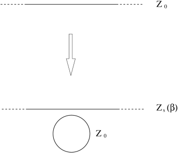
Figure 1: Representation of the compactification mechanism

2.2 Auxiliary fields

Let us now see how the use of auxiliary fields to exponentiate the constraints leads naturally to an alternative representation. The two $\delta$-functions require the introduction of two auxiliary fields, $\xi_{1}$ and $\xi_{2}$. which are just real (time-independent) variables in this case. Using the notation $Q_{1}\equiv q$ and $Q_{2}\equiv p$, we have

$$\prod_{a=1}^{2}\Big{\{}\delta\big{[}Q_{a}(\beta)-Q_{a}(0)\big{]}\Big{\}}\;=\;\int\frac{d^{2}\xi}{(2\pi)^{2}}\,e^{i\sum_{a=1}^{2}\xi_{a}\big{[}Q_{a}(\beta)-Q_{a}(0)\big{]}}\;.$$ (15)

Using this representation for the constraints and interchanging the order of integration for the multipliers and the phase space variables, the resulting expression for ${\mathcal{Z}}_{s}(\beta)$ may be written as follows:

$${\mathcal{Z}}_{s}(\beta) = {\mathcal{N}}^{-1}\,\int_{-\infty}^{\infty}\frac{d\xi_{1}}{2\pi}\int_{-\infty}^{\infty}\frac{d\xi_{2}}{2\pi}\int{\mathcal{D}}Q$$ (16)

$$\times e^{-{\mathcal{S}}(Q)\,+\,i\,\int_{-\infty}^{\infty}d\tau j_{a}(\tau)Q_{a}(\tau)}\;,$$

where $\mathcal{N}\equiv{\mathcal{Z}}_{0}$, and we have introduced the notation:

$$j_{a}(\tau)\equiv\xi_{a}\,\big{[}\delta(\tau-\beta)-\delta(\tau)\big{]}\;.$$ (17)

The phase-space measure has been written in terms of $Q$:

$${\mathcal{D}}Q\equiv\prod_{-\infty<\tau<\infty}\frac{dq(\tau)dp(\tau)}{2\pi}\;.$$ (18)

For the particular case of a harmonic oscillator with unit mass and frequency $\omega$, we have

$${\mathcal{S}}(Q)\;=\;{\mathcal{S}}_{0}(Q)\,=\,\frac{1}{2}\int_{-\infty}^{+\infty}d\tau\,Q_{a}(\tau)\widehat{{\mathcal{K}}}_{ab}Q_{a}(\tau)\;,$$ (19)

where $\widehat{\mathcal{K}}_{ab}$ are the elements of the $2\times 2$ operator matrix $\widehat{\mathcal{K}}$, given by:

$$\widehat{\mathcal{K}}\;=\;\left(\begin{array}[]{cc}\omega^{2}&i\frac{d}{d\tau}\\ -i\frac{d}{d\tau}&1\end{array}\right)\;.$$ (20)

Thus the integral over $Q$ is a Gaussian; it may therefore be written as follows:

$${\mathcal{Z}}_{s}(\beta)\;=\;2\pi\,{\mathcal{N}}^{-1}\,\big{(}\det\widehat{\mathcal{K}}\big{)}^{-\frac{1}{2}}\;\int\frac{d^{2}\xi}{(2\pi)^{2}}\,\,e^{-\frac{1}{2}\xi_{a}M_{ab}\xi_{b}}\;,$$ (21)

with

$$M\;\equiv\;\Omega(0_{+})\,+\Omega(0_{-})\,-\,\Omega(\beta)\,-\,\Omega(-\beta)\;,$$ (22)

where $\Omega(\tau)$ denotes the inverse of the operator ${\mathcal{K}}$ of (20); namely,

$$\widehat{\mathcal{K}}_{ac}\Omega_{cb}(\tau)\;=\;\delta_{ab}\,\delta(\tau)$$ (23)

where the $\Omega_{ab}$’s denote the matrix elements of $\Omega$.

The explicit form of this object may be easily found to be the following:

$$\Omega(\tau)\;\equiv\;\left(\begin{array}[]{cc}\frac{1}{2\omega}&\frac{i}{2}{\rm sgn}(\tau)\\ -\frac{i}{2}{\rm sgn}(\tau)&\frac{\omega}{2}\end{array}\right)\;e^{-\omega|\tau|}$$ (24)

(${\rm sgn}\equiv$ sign function).

Equation (24) can be used in (22), to see that:

$$M = \big{[}\Omega(0_{+})\,+\Omega(0_{-})\big{]}\,(1-e^{-\beta\omega})$$ (27)

$$= \left(\begin{array}[]{cc}\omega^{-1}&0\\ 0&\omega\end{array}\right)\;(n_{B}(\omega)+1)^{-1}\;,$$

where

$$n_{B}(\omega)\equiv(e^{\beta\omega}-1)^{-1}\$$ (28)

is the Bose-Einstein distribution function (with the zero of energy set at the ground state).

Finally, note that ${\mathcal{N}}$ exactly cancels the $\big{(}\det\widehat{\mathcal{K}}\big{)}^{-\frac{1}{2}}$ factor, and thus we arrive to a sort of ‘dual’ description for the partition function, as an integral over the $\xi_{a}$ variables:

$${\mathcal{Z}}_{s}(\beta)\;=\;\int\frac{d^{2}\xi}{2\pi}\,e^{-\frac{\omega^{-1}\,\xi_{1}^{2}\,+\;\omega\;\xi_{2}^{2}}{2[n_{B}(\omega)+1]}}\;.$$ (29)

This integral is over two real variables $\xi_{a}$, which are $0$-dimensional fields, one dimension less than the $0+1$ dimensional original theory. To interpret this integral we may compare it with the one corresponding to the classical statistical mechanics version of this system. To that end, we evaluate the partition function in the classical (high-temperature) limit. In that limit, we approximate the integrand accordingly to see that ${\mathcal{Z}}_{s}(\beta)$ becomes:

$${\mathcal{Z}}_{s}(\beta)\;\simeq\;\int\frac{d^{2}\xi}{2\pi}\,e^{-\beta H(\xi_{1},\xi_{2})}\;\;\;(\beta<<1)\;,$$ (30)

where:

$$H(\xi_{1},\xi_{2})\;\equiv\;\frac{1}{2}\big{(}\xi_{1}^{2}\,+\,\omega^{2}\xi_{2}^{2}\big{)}\;.$$ (31)

We see that (30) corresponds exactly to the classical partition function for a harmonic oscillator, when the identifications: $\xi_{1}=p$ (classical momentum), and $\xi_{2}=q$ (classical coordinate) are made

$${\mathcal{Z}}_{s}(\beta)\;\simeq\;\int\frac{dpdq}{2\pi}\,e^{-\beta\frac{1}{2}\big{(}p^{2}\,+\,\omega^{2}q^{2}\big{)}}\;\;\;(\beta<<1)\;.$$ (32)

On the other hand, had the exact form of the integral been kept (no approximation), we could still have written an expression similar to the classical partition function, albeit with an ‘effective Hamiltonian’ $H_{eff}(\xi_{1},\xi_{2})$:

$${\mathcal{Z}}_{s}(\beta)\;=\;\int\frac{d^{2}\xi}{2\pi}\,e^{-\beta H_{eff}(\xi_{1},\xi_{2})}\;,$$ (33)

where:

$$H_{eff}(\xi_{1},\xi_{2})\;\equiv\;\frac{1}{2\beta}\,\big{(}n_{B}(\omega)+1\big{)}^{-1}\,\big{(}\omega^{-1}\,\xi_{1}^{2}\,+\;\omega\;\xi_{2}^{2}\big{)}\;.$$ (34)

This shows that the quantum partition function may also be written as a classical one, by using a $\beta$-dependent Hamiltonian, which of course tends to its classical counterpart in the high-temperature limit.

By integrating out the auxiliary fields in the (exact) expression for the partition function (29), we obtain:

$${\mathcal{Z}}_{s}(\beta)\;=\;n_{B}(\omega)\,+\,1\;=\;\frac{1}{1\,-\,e^{-\beta\omega}}\;.$$ (35)

which is the correct result. In what follows, to simplify the notation, we shall omit writing the ‘$s$’ subscript in ${\mathcal{Z}}(\beta)$, assuming implicitly that one is dealing with the normal-ordered Hamiltonian.

An important fact that has emerged from an analysis of the classical (high-temperature) limit: the auxiliary fields do have a physical interpretation. The multiplier associated to the periodicity condition for $q$ plays the role of a classical momentum, while the one corresponding to the periodicity for the momentum becomes a generalization of the classical coordinate. The same interpretation might also be retained far from the classical limit, but then the Hamiltonian departs from the classical one, receiving quantum corrections.

This representation is also valid for interacting theories. To that effect, note that, even when the action ${\mathcal{S}}$ is not quadratic, we may still give a formal expression for the alternative representation. Indeed, denoting by ${\mathcal{Z}}(J)$ the zero-temperature generating functional of correlation functions of the canonical variables:

$${\mathcal{Z}}(J)\;=\;\int{\mathcal{D}}Q\,e^{-{\mathcal{S}}(Q)+\int_{-\infty}^{\infty}d\tau J_{a}(\tau)Q_{a}(\tau)}$$ (36)

and by ${\mathcal{W}}(J)$ the corresponding functional for connected ones, we see that

$${\mathcal{Z}}_{s}(\beta)\,=\,[{\mathcal{Z}}(0)]^{-1}\int\frac{d^{2}\xi}{(2\pi)^{2}}\,\exp\{{\mathcal{W}}\big{[}i\,j(\tau)\big{]}\}\;,$$ (37)

where, with our normalization conventions, ${\mathcal{Z}}(0)={\mathcal{Z}}_{0}$ (the vacuum functional for the interacting case).

Thus, a possible way to derive the effective Hamiltonian in the interacting case is to obtain first ${\mathcal{W}}[J]$, and then to replace the (arbitrary) source $J(\tau)$ by $ij(\tau)$, where $j(\tau)$ is the function of the auxiliary field defined in (17). Of course, ${\mathcal{W}}$ cannot be obtained exactly, except in very special cases. Otherwise, a suitable perturbative expansion can be used. In any case, ${\mathcal{W}}$ can be functionally expanded in powers of the source $J(\tau)$:

$${\mathcal{W}}[J]\,=\,{\mathcal{W}}[0]\,+\,\sum_{n=1}^{\infty}\frac{1}{n!}\int_{\tau_{1},\ldots,\tau_{n}}{\mathcal{W}}_{ab}^{(n)}(\tau_{1},\ldots,\tau_{n})J_{a_{1}}(\tau_{1})\ldots J_{a_{n}}(\tau_{n})$$ (38)

where each coefficient ${\mathcal{W}}^{(n)}$ is the $n$-point connected correlation function. The expansion above immediately yields an expansion for $H_{eff}$ in powers of the auxiliary fields. It is important to stress that this expansion is not necessarily a perturbative expansion. Indeed, the strength of each term is controlled by ${\mathcal{W}}^{(n)}$, which could even be exact (non-perturbative) in a coupling constant. To fix ideas, let us see what happens when one keeps only up to the $n=4$ term, assuming also that there is ${\mathcal{Q}}_{a}\to-{\mathcal{Q}}_{a}$ symmetry in ${\mathcal{S}}$. Then, we first see that the ${\mathcal{W}}[0]$ is cancelled by the ${\mathcal{N}}$ factor, and on the other hand we obtain

$${\mathcal{Z}}_{s}(\beta)\;=\;\int\frac{d^{2}\xi}{(2\pi)^{2}}\,e^{-\beta H_{eff}(\xi_{1},\xi_{2})}\;,$$ (39)

where

$$H_{eff} = \frac{1}{2\beta}\int_{\tau_{1},\tau_{2}}{\mathcal{W}}_{a_{1}a_{2}}^{(2)}(\tau_{1},\tau_{2})j_{a_{1}}(\tau_{1})j_{a_{2}}(\tau_{2})$$ (40)

$$- \frac{1}{4!\beta}\int_{\tau_{1},\tau_{2}}{\mathcal{W}}_{a_{1}a_{2}a_{3}a_{4}}^{(2)}(\tau_{1},\tau_{2},\tau_{3},\tau_{4})j_{a_{1}}(\tau_{1})j_{a_{2}}(\tau_{2})j_{a_{3}}(\tau_{3})j_{a_{4}}(\tau_{4})$$

$$+ \ldots$$

Using the explicit form of $j_{a}(\tau)$ in terms of the auxiliary fields, we see that:

$$H_{eff}\,=\,H_{eff}^{(2)}\,+\,H_{eff}^{(4)}\,+\,\ldots$$ (41)

where

$$H_{eff}^{(2)} = \frac{1}{2}{\mathcal{M}}^{(2)}_{ab}\xi_{a}\,\xi_{b}$$

$$H_{eff}^{(4)} = \frac{1}{4!}{\mathcal{M}}^{(4)}_{abcd}\;\xi_{a}\,\xi_{b}\,\xi_{c}\,\xi_{b}$$

$$\ldots = \ldots$$

$$H_{eff}^{(2k)} = \frac{1}{(2k)!}{\mathcal{M}}^{(2k)}_{a_{1}\ldots a_{2k}}\;\xi_{a_{1}}\ldots\xi_{a_{2k}}\;,$$ (42)

where the explicit forms of the coefficients ${\mathcal{M}}^{(2k)}$ in terms of ${\mathcal{W}}^{(2k)}$ may be found, after some algebra. For example ${\mathcal{M}}^{(2)}$ is a diagonal matrix:

$${\mathcal{M}}^{(2)}\,=\,\left(\begin{array}[]{cc}c_{1}&0\\ 0&c_{2}\end{array}\right)$$ (43)

where

$$c_{a}=\frac{1}{\beta}\,\int\frac{d\nu}{\pi}\;\big{(}1-e^{-i\nu\beta}\big{)}\,\tilde{\mathcal{W}}_{aa}(\nu)$$ (44)

(where the tilde denotes Fourier transform). It is immediate to realize that $c_{1}$ plays the role of an effective coefficient for the kinetic term ($\propto p^{2}$) in the effective Hamiltonian, while $c_{2}$ does introduce an effective quadratic potential. Note that they will, in general, depend on $\beta$, $\omega$, and on any additional coupling constant the system may have. For the harmonic oscillator case we have the rather simple form:

$$c_{1} = \frac{1}{\omega(n_{B}(\omega)+1)}$$

$$c_{2} = \frac{\omega}{n_{B}(\omega)+1}\;.$$ (45)

The quartic term involves ${\mathcal{M}}^{(4)}$, which may be written in terms of the connected $4$-point function:

$${\mathcal{M}}^{(4)}_{abcd}\;=\;\frac{1}{\beta}\,\Big{[}-{\mathcal{W}}^{(4)}_{abcd}(0,0,0,0)\,+\,4\,{\mathcal{W}}^{(4)}_{abcd}(\beta,\beta,\beta,0)$$

$$\,-\,6\,{\mathcal{W}}^{(4)}_{abcd}(\beta,\beta,0,0)\,+\,4\,{\mathcal{W}}^{(4)}_{abcd}(\beta,0,0,0)\,-\,{\mathcal{W}}^{(4)}_{abcd}(0,0,0,0)\Big{]}_{sym}$$ (46)

where the $sym$ suffix denotes symmetrization under simultaneous interchange of time arguments and discrete indices. Of course, this expression could also be written in Fourier space; we shall leave the analog of this term for the case of the real scalar field.

2.3 Generating functional

Now we proceed to the calculation of thermal correlation functions within the approach that we developed for the calculation of the partition function. To that end, we shall introduce the generating functional of correlation functions, to be denoted by ${\mathcal{Z}}_{s}(\beta,J)$, and ${\mathcal{W}}_{s}(\beta,J)\equiv\ln{\mathcal{Z}}_{s}(\beta,J)$ the generating functional of connected correlation functions. With these conventions, the connected correlation functions are given by:

$$\langle Q_{a_{1}}(\tau_{1})\ldots Q_{a_{n}}(\tau_{n})\rangle_{conn}\;=\;\Big{[}\frac{\delta^{n}{\mathcal{W}}_{s}(\beta,J)}{\delta J_{a_{1}}(\tau_{1})\,\ldots\,\delta J_{a_{n}}(\tau_{n})}\Big{]}_{J=0}\;.$$ (47)

From the previous subsection, we know that path integral expression for the generating functional shall be:

$${\mathcal{Z}}_{s}(\beta,J)\,=\,{\mathcal{N}}^{-1}\;\int\frac{d^{2}\xi}{2\pi}\;\int{\mathcal{D}}Q\,e^{-{\mathcal{S}}(Q)\,+\,\int_{-\infty}^{\infty}d\tau Q_{a}(\tau)(J_{a}(\tau)+ij_{a}(\tau))}$$ (48)

where ${\mathcal{S}}(Q)$ denotes the first-order form of the action.

Let us evaluate ${\mathcal{Z}}_{s}(\beta,J)$ explicitly for the case of the harmonic oscillator, where ${\mathcal{S}}$ is a quadratic form. The result of performing the Gaussian integral over $Q$, may be written in this case as follows:

$${\mathcal{Z}}_{s}(\beta,J)=\int\frac{d^{2}\xi}{2\pi}e^{\frac{1}{2}\int_{\infty}^{+\infty}d\tau_{1}\int_{\infty}^{+\infty}d\tau_{2}\,(J_{a}(\tau_{1})+ij_{a}(\tau_{1}))\Omega_{ab}(\tau_{1},\tau_{2})(J_{b}(\tau_{2})+ij_{b}(\tau_{2}))}\;.$$ (49)

Using the explicit form for $j_{a}$, we see that the expression above is equivalent to:

$${\mathcal{Z}}_{s}(\beta,J)\;=\;{\mathcal{Z}}_{s}(J)\int\frac{d^{2}\xi}{2\pi}e^{-\frac{1}{2}\xi_{a}M_{ab}\xi_{b}\,+\,i\xi_{a}N_{a}}$$ (50)

where ${\mathcal{Z}}_{s}(J)$ is the zero-temperature generating functional,

$${\mathcal{Z}}_{s}(J)=e^{\frac{1}{2}\int_{\infty}^{+\infty}d\tau_{1}\int_{\infty}^{+\infty}d\tau_{2}\,J_{a}(\tau_{1})\Omega_{ab}(\tau_{1},\tau_{2})J_{b}(\tau_{2})}$$ (51)

and

$$N_{a}\,\equiv\,\int_{-\infty}^{+\infty}d\tau\big{[}(\hat{\mathcal{K}}^{-1})_{ab}(\beta,\tau)-(\hat{\mathcal{K}}^{-1})_{ab}(0,\tau)\big{]}J_{b}(\tau)\;.$$ (52)

Integrating out the auxiliary fields, and recalling the results of the previous subsection,

$$Z_{s}(\beta,J)\,=\,Z(\beta)\;Z_{s}(J)\;e^{-\frac{1}{2}N_{a}\,[M^{-1}]_{ab}N_{b}}$$ (53)

where the $N_{a}$ are the functionals of $J_{a}$ defined in (52).

Neglecting a source-independent term (irrelevant for the calculation of correlation functions), the ${\mathcal{W}}$ generating functional will have the structure,

$${\mathcal{W}}_{s}(\beta,J)\,=\,\frac{1}{2}\int d\tau_{1}\int d\tau_{2}\,J_{a}(\tau_{1})G_{ab}(\tau_{1},\tau_{2})J_{b}(\tau_{2})$$ (54)

where $G_{ab}$ denotes the thermal correlation function:

$$G_{ab}(\tau_{1},\tau_{2})=G_{ab}(\tau_{1}-\tau_{2})=\langle Q_{a}(\tau_{1})Q_{b}(\tau_{2})\rangle\;,$$ (55)

whose structure we shall now write more explicitly. We first note that:

$$G_{ab}(\tau_{1},\tau_{2})\;=\;G^{(0)}_{ab}(\tau_{1},\tau_{2})-U^{(\beta)}_{ab}(\tau_{1},\tau_{2})$$ (56)

where $G^{(0)}$ is the zero-temperature correlation function while $U^{(\beta)}$ denotes a temperature-dependent piece.

We can write a more explicit form for the two terms that enter into the expression above for the correlation function. Indeed, for $G_{0}^{(\beta)}$ we have:

$$G^{(0)}(\tau)\;=\;\frac{e^{-\omega|\tau_{1}-\tau_{2}|}}{2\omega}\,\left(\begin{array}[]{cc}1&i\omega\\ -i\omega&\omega^{2}\end{array}\right)$$ (57)

while for $U^{(\beta)}$ we may use the following matrix representation:

$$U^{(\beta)}\,=\,\big{[}{\mathcal{K}}^{-1}(\tau_{1},\beta)-{\mathcal{K}}^{-1}(\tau_{1},0)\big{]}M^{-1}\big{[}{\mathcal{K}}^{-1}(\beta,\tau_{2})-{\mathcal{K}}^{-1}(0,\tau_{2})\big{]}$$ (58)

where ${\mathcal{K}}^{-1}(\tau,\tau^{\prime})$ denotes the kernel of the inverse of $\hat{\mathcal{K}}$. It is clear that $G^{(0)}$ is invariant under a translation in both time arguments. So is $U^{(\beta)}$, but one has to carry on the calculation in (58) to see that explicitly; indeed, assuming that both time arguments lie between $0$ and $\beta$, we have:

$$U^{(\beta)}(\tau_{1},\tau_{2})\;=\;-\frac{1}{2}\,n_{B}(\omega)\;\left(\begin{array}[]{cc}\frac{1}{\omega}(e^{-\omega\tau}+e^{\omega\tau})&i(e^{-\omega\tau}-e^{\omega\tau})\\ -i(e^{-\omega\tau}-e^{\omega\tau})&\omega(e^{-\omega\tau}+e^{\omega\tau})\end{array}\right)$$ (59)

where $\tau\equiv\tau_{1}-\tau_{2}$.

Thus, the thermal propagator only depends on $\tau$, the difference between the time arguments, and it is naturally defined on $[-\beta,\beta]$.

One is usually interested in the $\langle qq\rangle$ correlation function, which here we can immediately read off the general expressions above, since it corresponds to the $11$ matrix element. For $0<\tau\leq\beta$, we may derive the simpler expression:

$$G_{11}(\tau)=\frac{1}{2w}[(1+n_{B}(w))e^{-w\tau}+n_{B}(w)e^{w\tau}]\;,$$ (60)

which is the correct result . This is the unique solution to the differential equation:

$$(-\partial_{\tau}^{2}+\omega^{2})\,G_{11}(\tau)\;=\;\delta(\tau)$$ (61)

subject to the condition $G_{11}(\tau-\beta)=G_{11}(\tau)$. Moreover, we can understand that, in our construction, the zero-temperature part appears naturally as the propagator for the unconstrained system. On the other hand, $U^{(\beta)}$ is a solution to the homogeneous version of the equation above, and emerges as due to the boundary conditions.

So far, we have seen that the previous form correctly reproduces the free $2$-point function, for all the phase space variables, when both time arguments are inside the $[0,\beta]$ interval. A somewhat lengthy calculation shows that $G$ vanishes when one of its arguments is outside of that interval while the other is inside, and that it coincides with the $T=0$ function, $G^{(0)}$, when both are outside. Besides, in the last case, the $[0,\beta]$ interval is bypassed. More explicitly:

$$G(\tau_{1},\tau_{2})\;=\;\left\{\begin{array}[]{ccccc}0&{\rm if}&\tau_{1}>\beta&{\rm and}&0<\tau_{2}<\beta\\ G^{(0)}(\tau_{1},\tau_{2})&{\rm if}&\tau_{1}>\beta&{\rm and}&\tau_{2}>\beta\\ G^{(0)}(\tau_{1},\tau_{2})&{\rm if}&\tau_{1}<\beta&{\rm and}&\tau_{2}<\beta\\ G^{(0)}(\tau_{1}-\beta,\tau_{2})&{\rm if}&\tau_{1}>\beta&{\rm and}&\tau_{2}<0\end{array}\right.\;,$$ (62)

and the remaining cases follow from Bose symmetry.

This is an important property, since it allows us to perform a consistency check: indeed, coming back to the interacting case we considered in the previous subsection, one could have decided to perform the integrals in the opposite order, namely, first over the auxiliary fields and afterwards over $Q_{a}$. Then, the perturbative expansion would have involved the evaluation of Gaussian averages of the integration term, via Wick’s theorem, with $G$ as the fundamental contraction. Since the interaction term involves an infinite time interval, one produces not only the perturbative corrections to the partition function (when both times are inside $[0,\beta]$), but also a contribution that takes care of the normal order of the Hamiltonian (namely, when both arguments are outside of $[0,\beta]$.

3 Scalar field

The extension of the harmonic oscillator results to the QFT of a real scalar field $\varphi$ in $d+1$ (Euclidean) dimensions is quite straightforward. Let $\varphi(x)=\varphi(\tau,{\mathbf{x}})$ where $x=(\tau,{\mathbf{x}})\in{\mathbb{R}}^{(d+1)}$, $\tau\in{\mathbb{R}}$ and ${\mathbf{x}}\in{\mathbb{R}}^{(d)}$. Proceeding along the same lines as for the case of a single degree of freedom, we consider first the free case.

3.1 Free partition function

The free Euclidean action in terms of the phase-space variables ${\mathcal{S}}_{0}$, is in this case given by:

$${\mathcal{S}}_{0}\,=\,\int d^{d+1}x\,\Big{[}-i\pi\partial_{\tau}\varphi+{\mathcal{H}}_{0}(\pi,\varphi)\Big{]}\;,$$ (63)

with

$${\mathcal{H}}_{0}(\pi,\varphi)\;\equiv\;\frac{1}{2}\Big{[}\pi^{2}\,+\,|{\mathbf{\nabla}}\varphi|^{2}+m^{2}\varphi^{2}\Big{]}\;.$$ (64)

We then have to implement the periodic boundary conditions both for $\varphi(\tau,{\mathbf{x}})$ and its canonical momentum $\pi(\tau,{\mathbf{x}})$

$$\varphi\left(\beta,{\mathbf{x}}\right)\,=\,\varphi\left(0,{\mathbf{x}}\right)\;,\;\;\;\pi\left(\beta,{\mathbf{x}}\right)\,=\,\pi\left(0,{\mathbf{x}}\right)\;,\;\;\forall\,{\mathbf{x}}\,\in{\mathbb{R}}^{(d)}\;,$$ (65)

which requires the introduction of two time-independent Lagrange multiplier fields: $\xi_{a}({\mathbf{x}})$, $a=1,\,2$. Defining a two-component field $\Phi=(\Phi_{a})$, $a=1,\,2$, such that $\Phi_{1}=\varphi$ and $\Phi_{2}=\pi$, an analogous procedure to the one followed for the harmonic oscillator yields, for the free partition function ${\mathcal{Z}}_{0}(\beta)$:

$${\mathcal{Z}}_{0}(\beta)\;=\;{\mathcal{N}}^{-1}\,\int\,{\mathcal{D}}\xi\,\int{\mathcal{D}}\Phi\;e^{-\frac{1}{2}\int d^{d+1}x\,\Phi_{a}{\hat{\mathcal{K}}}_{ab}\Phi_{b}\,+\,i\,\int d^{d+1}xj_{a}\Phi_{a}}\;,$$ (66)

where $j_{a}(x)\equiv\xi_{a}({\mathbf{x}})\big{[}\delta(\tau-\beta)-\delta(\tau)\big{]}$ and:

$${\widehat{\mathcal{K}}}\;=\;\left(\begin{array}[]{cc}{\hat{h}}^{2}&i\frac{\partial}{\partial\tau}\\ -i\frac{\partial}{\partial\tau}&1\end{array}\right)\;,$$ (67)

where we have introduced ${\hat{h}}\equiv\sqrt{-\nabla^{2}+m^{2}}$, the first-quantized energy operator for massive scalar particles. Performing the integral over $\Phi$, yields the partition function in terms of the Lagrange multipliers:

$${\mathcal{Z}}_{0}(\beta)\;=\;\int{\mathcal{D}}\xi\,e^{-\frac{1}{2}\int d^{d}x\int d^{d}y\,\xi_{a}({\mathbf{x}})\;\langle{\mathbf{x}}|{\hat{M}}_{ab}|{\mathbf{y}}\rangle\;\xi_{b}({\mathbf{y}})}\;,$$ (68)

with ${\hat{M}}\equiv{\hat{\Omega}}(0_{+})+{\hat{\Omega}}(0_{-})-{\hat{\Omega}}(\beta)-{\hat{\Omega}}(-\beta)$ and

$${\hat{\Omega}}(\tau)\;\equiv\;\left(\begin{array}[]{cc}\frac{1}{2}{\hat{h}}^{-1}&\frac{i}{2}{\rm sgn}(\tau)\\ -\frac{i}{2}{\rm sgn}(\tau)&\frac{1}{2}{\hat{h}}\end{array}\right)\;e^{-{\hat{h}}|\tau|}\;.$$ (69)

Then,

$${\hat{M}}\;\equiv\;\left(\begin{array}[]{cc}{\hat{h}}^{-1}&0\\ 0&{\hat{h}}\end{array}\right)\;({\hat{n}}_{B}+1)^{-1}\;,$$ (70)

where

$${\hat{n}}_{B}\;\equiv\;\frac{1}{e^{\beta{\hat{h}}}-1}\;.$$ (71)

Coming back to the expression for ${\mathcal{Z}}_{0}(\beta)$, we see that:

$${\mathcal{Z}}_{0}(\beta) = \int{\mathcal{D}}\xi\,\exp\Big{\{}-\frac{1}{2}\int d^{d}x\int d^{d}y\big{[}\xi_{1}({\mathbf{x}})\;\langle{\mathbf{x}}|{\hat{h}}^{-1}\,({\hat{n}}_{B}+1)^{-1}|{\mathbf{y}}\rangle\;\xi_{1}({\mathbf{y}})$$ (72)

$$+ \xi_{2}({\mathbf{x}})\;\langle{\mathbf{x}}|{\hat{h}}\,({\hat{n}}_{B}+1)^{-1}|{\mathbf{y}}\rangle\;\xi_{2}({\mathbf{y}})\big{]}\Big{\}}\;.$$

By a simple field redefinition, we see that:

$${\mathcal{Z}}_{0}(\beta)\;=\;\det\big{(}{\hat{n}}_{B}+1\big{)}$$ (73)

which can be evaluated in the basis of eigenstates of momentum to yield:

$${\mathcal{Z}}_{0}(\beta)\;=\;\prod_{\mathbf{k}}\big{[}n_{B}(E_{\mathbf{k}})+1\big{]}$$ (74)

where $E_{\mathbf{k}}\equiv\sqrt{{\mathbf{k}}^{2}+m^{2}}$. The free-energy density, $F_{0}(\beta)$, is of course:

$$F_{0}(\beta)\;=\;\frac{1}{\beta}\,\int\frac{d^{d}k}{(2\pi)^{d}}\,\ln\big{(}1\,-\,e^{-\beta E_{\mathbf{k}}}\big{)}\;.$$ (75)

In the classical, high-temperature limit, the path integral for the partition function becomes:

$${\mathcal{Z}}_{0}(\beta)\;\simeq\;\int{\mathcal{D}}\xi\,e^{-\beta\;H(\xi)}\;,$$ (76)

where:

$$H(\xi)\;=\;\frac{1}{2}\int d^{d}x\big{[}\xi_{1}^{2}({\mathbf{x}})\,+\,|{\mathbf{\nabla}}\xi_{2}({\mathbf{x}})|^{2}\,+\,m^{2}\,\xi_{2}^{2}({\mathbf{x}})\Big{]}\;.$$ (77)

This is, again, the usual classical expression for the partition function, with the Lagrange multipliers playing the role of phase space variables, and the integration measure being the corresponding Liouville measure. Besides, it is clear that the representation (72) always involves static fields, unlike in the Matsubara formalism. The price to pay for this ‘dimensional reduction’ is that the resulting ‘action’ (the exponent of the functional to be integrated) is spatially non local. It becomes local only in the high-temperature limit.

3.2 Quadratic approximation

Let us study here a simple yet illuminating example where this approach allows one to use non-perturbative $T=0$ information about a system as input for the finite temperature partition function in a quite simple way. So we assume that we know the exact $2$-point function ${\mathcal{W}}^{(2)}_{ab}$ at zero temperature. To be precise, since the Hamiltonian is quadratic in the canonical momentum, we only need to know ${\mathcal{W}}^{(2)}_{11}$, since it is possible to show that when one of the fields is replaced by the canonical momentum, the result is multiplied by the corresponding frequency (in Fourier space). Indeed, this can be shown, for example, by performing the exact integral over the canonical momentum.

Then the effective Hamiltonian corresponding to this term has the form:

$$H_{eff}(\xi)\,=\,\frac{1}{2}\int_{{\mathbf{x}},{\mathbf{y}}}\Big{[}\xi_{1}({\mathbf{x}})C_{1}({\mathbf{x}}-{\mathbf{y}})\xi_{1}({\mathbf{y}})\,+\,\xi_{2}({\mathbf{x}})C_{2}({\mathbf{x}}-{\mathbf{y}})\xi_{2}({\mathbf{y}})\Big{]}$$ (78)

where the Fourier transforms of the coefficients $C_{1}$ and $C_{2}$ are

$${\tilde{C}}_{1}({\mathbf{k}}) = \frac{1}{\beta}\,\int\frac{dk_{0}}{\pi}\;\big{(}1-e^{-i\beta k_{0}}\big{)}\,\tilde{\mathcal{W}}_{11}(k_{0},{\mathbf{k}})$$

$${\tilde{C}}_{2}({\mathbf{k}}) = \frac{1}{\beta}\,\int\frac{dk_{0}}{\pi}\;\big{(}1-e^{-i\beta k_{0}}\big{)}\,k_{0}^{2}\,\tilde{\mathcal{W}}_{11}(k_{0},{\mathbf{k}})\;.$$ (79)

Note that these two coefficients that determine the contribution of the quadratic term to the partition function, could be rather involved functions of the functions of a coupling constant, since we are not perturbing but just assuming that we only consider the information contained in the full propagator.

Assuming now that the exact propagator is such that only one particle, with energy $E({\mathbf{k}})$, exists, one knows that there can only be poles associated to them in $\widetilde{\mathcal{W}}_{11}$. Moreover, we assume that, as usual, renormalization conditions have been imposed such that the residue is $1$. Then we obtain:

$${\tilde{C}}_{1}({\mathbf{k}}) = \frac{1}{\beta E({\mathbf{k}})}\,\big{(}1-e^{-\beta E({\mathbf{k}})}\big{)}$$

$${\tilde{C}}_{2}({\mathbf{k}}) = \frac{E({\mathbf{k}})}{\beta}\,\big{(}1-e^{-\beta E({\mathbf{k}})}\big{)}\;,$$ (80)

and the partition function becomes:

$${\mathcal{Z}}_{s}(\beta)\,=\,\prod_{\mathbf{k}}\frac{1}{1-e^{-\beta E({\mathbf{k}})}}\;,$$ (81)

which is of course the one of an ideal Bose gas. But the important difference is that one is obtaining it by putting the information contained in the knowledge of the non-perturbative spectrum. It could be the case, for example, of a model where the mass is generated by a non-perturbative mechanism. Or one could have a theory with more than one pole, corresponding for example to different bound states. These non-trivial poles, obtained in the $T=0$ theory are then directly taken into account by this contribution, as the first terms in an expansion in powers of the auxiliary fields. Of course, one has to include, in general, also non-quadratic terms. The quadratic approximation could be justified, for example, within the context of a large-$N$ approximation.

3.3 Perturbation theory

We study here the alternative representation for the partition function in an interacting theory. For the sake of clarity, we present this topic within the context of a concrete example: the real scalar field in $3+1$ dimensions, with a self-interaction of the quartic type. The action is then

$${\mathcal{S}}\;=\;{\mathcal{S}}_{0}\,+\,{\mathcal{S}}_{I}\;\;,\;\;\;\;{\mathcal{S}}_{I}\,=\,\frac{\lambda}{4!}\int d^{4}x\,\varphi^{4}(x)\;.$$ (82)

As in the standard formulation, we want to calculate ${\mathcal{Z}}(\beta)$ in a power series of the coupling constant, $\lambda$. It should be clear that the proper way to do that here is to calculate ${\mathcal{W}}[J]$ to the desired order, and from there to obtain the corresponding effective Hamiltonian. The resulting expression for the partition function as a functional integral over the auxiliary fields can then also be expanded (up to the same order ${\mathcal{W}}[J]$ was calculated). In the course of such a program one has to face the issue of the UV infinites that pop up in the calculation of loop diagrams for the (zero-temperature) object ${\mathcal{W}}[J]$. We shall assume that all those infinities are renormalized in the usual way at zero temperature. In particular, our $T=0$ vertices are normal ordered, so that the zero-temperature tadpoles are, to begin with, absent. The finite-temperature tadpoles will, nevertheless, appear in the alternative description, as we shall see. Namely, the functional integral in terms of the auxiliary fields is UV finite. In this way, the thermal corrections are completely disentangled from the issue of renormalization.

We now study the problem of calculating the effective Hamiltonian in terms of the perturbative expansion for ${\mathcal{W}}[J]$. As in the case of one degree of freedom, the effective Hamiltonian is related to ${\mathcal{W}}[J]$ by:

$$H_{eff}(\xi)\;=\;-\frac{1}{\beta}\;{\mathcal{W}}[ij(x)]$$ (83)

where ${\mathcal{W}}[J]$ is the generating functional of connected correlation functions $\Phi_{a}$, at $T=0$. Moreover, we shall assume that, in the previous expression, ${\mathcal{W}}[0]\equiv 0$, since any vacuum contributions would be cancelled by the normalization factor ${\mathcal{N}}$.

The perturbative expansion of ${\mathcal{W}}$ will be denoted by ${\mathcal{W}}\,=\,{\mathcal{W}}^{(0)}+{\mathcal{W}}^{(I)}$, with

$${\mathcal{W}}_{I}[J]\;=\;{\mathcal{W}}^{(1)}[J]\,+\,{\mathcal{W}}^{(2)}[J]\,+\,\ldots$$ (84)

where the index denotes the order in $\lambda$ of the corresponding term. This yields the corresponding expansion for the effective Hamiltonian, $H_{eff}\,=\,H_{eff}^{(0)}+H_{eff}^{(I)}$, and one can then find corrections to the partition function, or the free energy $F=-\frac{1}{\beta}\ln{\mathcal{Z}}$, by evaluating the corresponding Gaussian averages. Indeed,

$$F(\beta)\,=\,F^{(0)}(\beta)+F^{(I)}(\beta)$$ (85)

where

$$F^{(I)}(\beta)\,=\,-\frac{1}{\beta}\ln\langle e^{-\beta H_{eff}^{(I)}(\xi)}\rangle$$ (86)

where the average symbol is defined by the quadratic weight:

$$\langle\ldots\rangle\;\equiv\;\frac{\int{\mathcal{D}}\xi\ldots e^{-\beta H_{eff}^{(0)}(\xi)}}{{\mathcal{Z}}_{0}(\beta)}\;.$$ (87)

To fix ideas, we do that first for the simplest non-trivial order, i.e., $\lambda$. Then one has the first-order contribution to $F$:

$$F^{(1)}(\beta)\,=\,\langle H_{eff}^{(1)}(\xi)\rangle\;,$$ (88)

where the Gaussian average requires the knowledge of the elementary averages which involve two auxiliary fields. The only non-trivial ones are:

$$\langle\xi_{1}({\mathbf{x}})\xi_{1}({\mathbf{y}})\rangle = \int\frac{d^{3}k}{(2\pi)^{3}}e^{i{\mathbf{k}}\cdot({\mathbf{x}}-{\mathbf{y}})}\frac{\omega({\mathbf{k}})}{1-e^{-\beta\omega({\mathbf{k}})}}$$

$$\langle\xi_{2}({\mathbf{x}})\xi_{2}({\mathbf{y}})\rangle = \int\frac{d^{3}k}{(2\pi)^{3}}e^{i{\mathbf{k}}\cdot({\mathbf{x}}-{\mathbf{y}})}\frac{1}{\omega({\mathbf{k}})(1-e^{-\beta\omega({\mathbf{k}})})}\;.$$ (89)

On the other hand, a standard $T=0$ calculation shows that the first-order term in the expansion of ${\mathcal{W}}$ is:

$${\mathcal{W}}^{(1)}[J]\;=\;-\frac{\lambda}{4!}\,\int d^{4}x\Big{[}\int d^{4}y\sum_{a}G^{(0)}_{1a}(x-y)J_{a}(y)\Big{]}^{4}\;,$$ (90)

where $G^{(0)}_{ab}(x-y)$ is the free $T=0$ propagator for the real scalar field and its canonical momentum, namely

$$G^{(0)}_{ab}(x-y)\,=\,\langle\Phi_{a}(x)\,\Phi_{b}(y)\rangle\;,$$ (91)

which may be conveniently represented in terms of its Fourier transforms ${\tilde{G}}^{(0)}_{ab}(k)$, in a matrix representation where ($1$ corresponds to $\varphi$ and $2$ to $\pi$):

$${\tilde{G}}^{(0)}(k)\,=\,\frac{1}{k^{2}+m^{2}}\left(\begin{array}[]{cc}1&ik_{0}\\ -ik_{0}&k_{0}^{2}\end{array}\right)\;.$$ (92)

Using now the rule that maps terms in the expansion for ${\mathcal{W}}$ into like ones for $H_{eff}$, we see that:

$$H^{(1)}_{eff}(\xi) = \frac{\lambda}{4!\beta}\,\int d^{4}x\Big{[}\int d^{4}y\sum_{a}G^{(0)}_{1a}(x-y)$$ (93)

$$\times \xi_{a}({\mathbf{y}})(\delta(y_{0}-\beta)-\delta(y_{0}))\Big{]}^{4}\;.$$

Then, using tildes to denote the Fourier transforms of the auxiliary fields, we see that each one of the factors that appear integrated over $x$ above, can be put in the following form:

$$\int d^{4}y\,\sum_{a}G^{(0)}_{1a}(x-y)\xi_{a}({\mathbf{y}})\big{[}\delta(y_{0}-\beta)-\delta(y_{0})\big{]}$$

$$= \int\frac{d^{3}k}{(2\pi)^{3}}\,\frac{1}{2\omega({\mathbf{k}})}\,e^{i{\mathbf{k}}\cdot{\mathbf{x}}}\big{[}e^{-\omega({\mathbf{k}})|x_{0}-\beta|}-e^{-\omega({\mathbf{k}})|x_{0}|}\big{]}{\tilde{\xi}}_{1}({\mathbf{k}})$$ (94)

$$+ \int\frac{d^{3}k}{(2\pi)^{3}}\,e^{i{\mathbf{k}}\cdot{\mathbf{x}}}\frac{1}{2}\big{[}\sigma(x_{0})e^{-\omega({\mathbf{k}})|x_{0}|}-\sigma(x_{0}-\beta)e^{-\omega({\mathbf{k}})|x_{0}-\beta|}\big{]}{\tilde{\xi}}_{2}({\mathbf{k}})\;,$$

where $\sigma(x)$ denotes the sign of $x$.

Introducing the expression above into (93) we find, in a natural extension of the notation used for the case of one degree of freedom:

$$H^{(1)}_{eff}(\xi) = \frac{1}{4!}\,\int\Big{[}\prod_{i=1}^{4}\frac{d^{3}k_{i}}{(2\pi)^{3}}\Big{]}\,(2\pi)^{3}\delta^{(3)}\big{(}\sum_{i=1}^{4}{\mathbf{k}}_{i}\big{)}\,{\mathcal{H}}^{(4,1)}_{a_{1}\ldots a_{4}}({\mathbf{k}}_{1},\ldots,{\mathbf{k}}_{4})$$ (95)

$$\times {\tilde{\xi}}_{a_{1}}({\mathbf{k}}_{1})\ldots{\tilde{\xi}}_{a_{4}}({\mathbf{k}}_{4})$$

where ${\mathcal{H}}^{(4,1)}$ is the kernel for a quartic term; the $`1^{\prime}$ has been written to pinpoint the fact that it has been calculated to the first order. The explicit form of the kernel elements depends of course on the indices considered. Modulo permutations, the only inequivalent possibilities are summarized in the following results:

$${\mathcal{H}}^{(4,1)}_{1111}({\mathbf{k}}_{1},{\mathbf{k}}_{2},{\mathbf{k}}_{3},{\mathbf{k}}_{4})\,=\,\lambda\,\int\Big{(}\prod_{i=1}^{4}\frac{d\nu_{i}}{2\pi}\Big{)}\,2\pi\,\delta(\sum_{j=1}^{4}\nu_{j})\,\prod_{l=1}^{4}\Big{[}\frac{e^{-i\beta\nu_{l}}-1}{\nu_{l}^{2}+\omega^{2}({\mathbf{k}}_{l})}\Big{]}\;,$$ (96)

$${\mathcal{H}}^{(4,1)}_{1112}({\mathbf{k}}_{1},{\mathbf{k}}_{2},{\mathbf{k}}_{3},{\mathbf{k}}_{4}) = \lambda\,\int\Big{(}\prod_{i=1}^{4}\frac{d\nu_{i}}{2\pi}\Big{)}\,2\pi\,\delta(\sum_{j=1}^{4}\nu_{j})$$ (97)

$$\times \prod_{l=1}^{3}\Big{[}\frac{e^{-i\beta\nu_{l}}-1}{\nu_{l}^{2}+\omega^{2}({\mathbf{k}}_{l})}\Big{]}\;\;\frac{i\nu_{4}\big{(}e^{-i\beta\nu_{4}}-1\big{)}}{\nu_{4}^{2}+\omega^{2}({\mathbf{k}}_{4})}$$

$${\mathcal{H}}^{(4,1)}_{1122}({\mathbf{k}}_{1},{\mathbf{k}}_{2},{\mathbf{k}}_{3},{\mathbf{k}}_{4}) = \lambda\,\int\Big{(}\prod_{i=1}^{4}\frac{d\nu_{i}}{2\pi}\Big{)}\,2\pi\,\delta(\sum_{j=1}^{4}\nu_{j})$$ (98)

$$\times \prod_{l=1}^{2}\Big{[}\frac{e^{-i\beta\nu_{l}}-1}{\nu_{l}^{2}+\omega^{2}({\mathbf{k}}_{l})}\Big{]}\;\;\prod_{r=3}^{4}\Big{[}\frac{i\nu_{r}\big{(}e^{-i\beta\nu_{r}}-1\big{)}}{\nu_{r}^{2}+\omega^{2}({\mathbf{k}}_{r})}\Big{]}\;,$$

$${\mathcal{H}}^{(4,1)}_{1222}({\mathbf{k}}_{1},{\mathbf{k}}_{2},{\mathbf{k}}_{3},{\mathbf{k}}_{4}) = \lambda\,\int\Big{(}\prod_{i=1}^{4}\frac{d\nu_{i}}{2\pi}\Big{)}\,2\pi\,\delta(\sum_{j=1}^{4}\nu_{j})$$ (99)

$$\times \frac{e^{-i\beta\nu_{1}}-1}{\nu_{1}^{2}+\omega^{2}({\mathbf{k}}_{1})}\;\;\prod_{r=2}^{4}\Big{[}\frac{i\nu_{r}\big{(}e^{-i\beta\nu_{r}}-1\big{)}}{\nu_{r}^{2}+\omega^{2}({\mathbf{k}}_{r})}\Big{]}\;,$$

and

$${\mathcal{H}}^{(4,1)}_{2222}({\mathbf{k}}_{1},{\mathbf{k}}_{2},{\mathbf{k}}_{3},{\mathbf{k}}_{4})\,=\,\lambda\,\int\Big{(}\prod_{i=1}^{4}\frac{d\nu_{i}}{2\pi}\Big{)}\,2\pi\,\delta(\sum_{j=1}^{4}\nu_{j})\,\prod_{l=1}^{4}\Big{[}\frac{i\nu_{l}\big{(}e^{-i\beta\nu_{l}}-1\big{)}}{\nu_{l}^{2}+\omega^{2}({\mathbf{k}}_{l})}\Big{]}\;.$$ (100)

Upon application of Wick’s theorem for the calculation of the average of the first order effective Hamiltonian, we see that only the terms with an even number of legs for each field yields a non-vanishing contraction; namely, only the terms ${\mathcal{H}}^{(4,1)}_{1111}$, ${\mathcal{H}}^{(4,1)}_{1122}$, ${\mathcal{H}}^{(4,1)}_{2222}$ enter into the calculation. Besides, the first and third of these carry a factor of $3$ because of the number of unequivalent contractions, while for the second one there is a $6$ due to the different permutations of the (different) indices.

Using the explicit form of the contractions, and integrating over the frequencies, one sees, after a somewhat lengthy, but nevertheless straightforward calculation, that the proper result is obtained. Namely,

$$F^{(1)}\,=\,\frac{\lambda}{8\beta}\,V\,\Big{(}\int\frac{d^{3}k}{(2\pi)^{3}}\frac{1}{\omega({\mathbf{k}})}n_{B}(\omega({\mathbf{k}}))\Big{)}^{2}\;,$$ (101)

where $V$ is the spatial volume of the system.

3.4 Generating functional

Including a source in equation (66) it is straightforward to obtain the generating functional for the scalar field in $d+1$ dimensions in a analogous form than for $0+1$ dimensional theory. Working in Fourier space for the spatial coordinates, we see that the entire $0+1$ dimensional procedure applies. Then $G_{ab}(x,y)$, the correlation function for the scalar field and its canonical momentum becomes:

$$G_{ab}(x,y)\,=\,G_{ab}^{(0)}(x-y)-U^{(\beta)}_{ab}(x-y)\;,$$ (102)

where $G_{ab}^{(0)}(x-y)$ is the zero temperature correlation function, whereas $U_{ab}^{(\beta)}(x-y)$ is a temperature dependent function.

The explicit form of these functions is:

$$G_{ab}^{(0)}(x-y)\,=\,\int\frac{d^{d}\mathbf{k}}{(2\pi)^{d}}\,e^{i\mathbf{k}\,(\mathbf{x}-\mathbf{y})}\,\,G_{ab}^{(0)}(\mathbf{k},\tau)$$ (103)

where:

$$G_{ab}^{(0)}(\mathbf{p},\tau)\,=\,\frac{e^{-\omega_{\mathbf{k}}\tau}}{2\omega_{\mathbf{k}}}\left(\begin{array}[]{cc}1&i\omega_{\mathbf{k}}\\ -i\omega_{\mathbf{k}}&\omega^{2}_{\mathbf{k}}\end{array}\right)\;,$$ (104)

and:

$$U^{(\beta)}({\mathbf{k}},\tau)\,=\,-\frac{n_{B}(\omega_{\mathbf{k}})}{2}\left(\begin{array}[]{cc}\frac{e^{\omega_{\mathbf{k}}\tau}+e^{-\omega_{\mathbf{k}}\tau}}{\omega_{\mathbf{k}}}&-i\big{(}e^{\omega_{\mathbf{k}}\tau}-e^{-\omega_{\mathbf{k}}\tau}\big{)}\\ -i\big{(}e^{\omega_{\mathbf{k}}\tau}-e^{-\omega_{\mathbf{k}}\tau}\big{)}&\omega_{\mathbf{k}}\big{(}e^{\omega_{\mathbf{k}}\tau}+e^{-\omega_{\mathbf{k}}\tau}\big{)}\end{array}\right)\;,$$ (105)

which are exactly equal to the $0+1$ dimensional case equations on which we have to replace $w$ by $\omega_{\mathbf{k}}=\sqrt{\mathbf{k}^{2}+m^{2}}$.

4 Dirac field

The final example we consider is a massive Dirac field in $d+1$ spacetime dimensions. The procedure will be essentially the same as for the real scalar field, once the relevant kinematical differences are taken into account. The action $S_{0}^{f}$ for the free case is given by $S_{0}^{f}=\int d^{d+1}x\bar{\psi}(\not\!\partial+m)\psi$ where $\not\!\partial=\gamma_{\mu}\partial_{\mu}$, $\gamma_{\mu}^{\dagger}=\gamma_{\mu}$ and $\{\gamma_{\mu},\gamma_{\nu}\}=2\delta_{\mu\nu}$.

We then impose antiperiodic conditions for both fields:

$$\psi\left(\beta,{\mathbf{x}}\right)\,=\,-{\psi}\left(0,{\mathbf{x}}\right)\;,\;\;\bar{\psi}\left(\beta,{\mathbf{x}}\right)\,=\,-\bar{\psi}\left(0,{\mathbf{x}}\right)$$ (106)

as constraints on the Grassmann fields. Those conditions lead to the introduction of the two $\delta-$functions:

$${\mathcal{Z}}_{0}^{f}(\beta) = \int\,{\mathcal{D}}\psi{\mathcal{D}}\bar{\psi}\,\delta\big{(}\psi(\beta,{\mathbf{x}})+\psi(0,{\mathbf{x}})\big{)}\;\delta\big{(}\bar{\psi}(\beta,{\mathbf{x}})+\bar{\psi}(0,{\mathbf{x}})\big{)}$$ (107)

$$\times \exp\Big{[}-S_{0}^{f}(\bar{\psi},\psi)\Big{]}\;.$$

Since the Dirac action is of the first-order, the introduction of two constraints, and two Lagrange multipliers, appears in an even more natural way than for the previous case. Those auxiliary fields, denoted by $\chi(\mathbf{x})$ and $\bar{\chi}(\mathbf{x})$ must be time-independent Grassmann spinors. The resulting expression for ${\mathcal{Z}}_{0}^{f}(\beta)$ is then

$${\mathcal{Z}}_{0}^{f}(\beta)\;=\;{\mathcal{N}}^{-1}\,\int\,{\mathcal{D}}\chi{\mathcal{D}}\bar{\chi}{\mathcal{D}}\psi{\mathcal{D}}\bar{\psi}\,e^{-S_{0}^{f}(\bar{\psi},\psi)+i\,\int d^{d+1}x\,(\bar{\eta}\psi+\bar{\psi}\eta)},$$ (108)

where $\eta$ and $\bar{\eta}$ are (Grassmann) sources depending on $\chi$ and $\bar{\chi}$ through the relations:

$$\eta(x)\,=\,\chi({\mathbf{x}})\big{[}\delta(\tau-\beta)+\delta(\tau)\big{]}\;,\;\;\;\bar{\eta}(x)\,=\,\bar{\chi}({\mathbf{x}})\big{[}\delta(\tau-\beta)+\delta(\tau)\big{]}\;.$$ (109)

Integrating out $\psi,\bar{\psi}$, we arrive to:

$${\mathcal{Z}}_{0}^{f}(\beta)\;=\;\int\,{\mathcal{D}}\chi{\mathcal{D}}\bar{\chi}\,\exp\Big{[}-\beta H_{eff}\big{(}\bar{\chi},\chi\big{)}\Big{]}$$ (110)

where

$$H_{eff}\big{(}\bar{\chi},\chi\big{)}=\int d^{d}x\,\int d^{d}y\,\bar{\chi}({\mathbf{x}})H^{(2)}\big{(}{\mathbf{x}},{\mathbf{y}}\big{)}\chi({\mathbf{y}})$$ (111)

with:

$$H^{(2)}\big{(}{\mathbf{x}},{\mathbf{y}}\big{)}\;=\;\langle\mathbf{x},0|(\not\!\partial+m)^{-1}|\mathbf{y},0\rangle+\langle\mathbf{x},\beta|(\not\!\partial+m)^{-1}|\mathbf{y},\beta\rangle$$

$$+\,\langle\mathbf{x},0|(\not\!\partial+m)^{-1}|\mathbf{y},\beta\rangle+\langle\mathbf{x},\beta|(\not\!\partial+m)^{-1}|\mathbf{y},0\rangle$$

$$=\,\frac{1}{\beta}\,\Big{[}2\,S_{f}\big{(}0,\mathbf{x}-\mathbf{y}\big{)}+S_{f}\big{(}\beta,\mathbf{x}-\mathbf{y}\big{)}+S_{f}\big{(}-\beta,\mathbf{x}-\mathbf{y}\big{)}\Big{]}.$$ (112)

On the last line, $S_{f}$, denotes the Dirac propagator. A quite straightforward calculation shows that

$$H\big{(}{\mathbf{x}},{\mathbf{y}}\big{)}=\frac{1}{\beta}\,\langle\mathbf{x}|\hat{u}(1-\hat{n}_{F})^{-1}|\mathbf{y}\rangle$$ (113)

where $\hat{n}_{F}\equiv\Big{(}1+e^{\beta\hat{n}}\Big{)}^{-1}$ is the Fermi-Dirac distribution function, written in terms of $\hat{h}$, the energy operator (defined identically to its real scalar field counterpart); $\hat{u}$ is a unitary operator, defined as

$$\hat{u}\;\equiv\;\frac{\hat{h}_{D}}{\hat{h}}\,,\;\;\hat{h}_{D}\equiv{\mathbf{\gamma}}\,\cdot\,{\mathbf{\nabla}}+m\;.$$ (114)

Then we verify that:

$${\mathcal{Z}}_{0}^{f}(\beta)\;=\;\det\hat{u}\;{\det}^{-1}\big{[}(1-\hat{n}_{F})\,\mathbf{I}\big{]}\;,$$ (115)

($\mathbf{I}\,\equiv$ identity matrix in the representation of Dirac’s algebra)

$${\mathcal{Z}}_{0}^{f}(\beta)\;=\;\left\{\prod_{\vec{p}}\Big{[}1+e^{-\beta E(\vec{p})}\Big{]}\right\}^{r_{d}}$$ (116)

with $E({\mathbf{p}})=\sqrt{{\mathbf{p}}^{2}+m^{2}}$ and $r_{d}\,\equiv$ dimension of the representation (we have used the fact that $\det\hat{u}=1$).

Again, the procedure has produced the right result for the partition function, with a normal-ordered Hamiltonian. On the other hand, for a Dirac field in a static external background corresponding to a minimally coupled Abelian gauge field the $A_{0}=0$ gauge, we have

$$S^{f}(\bar{\psi},\psi,A)\;=\;\int d^{d+1}x\,\Big{[}\bar{\psi}(x)\big{(}\not\!\partial+i\,e\,{\mathbf{\gamma}}\cdot{\mathbf{A}}({\mathbf{x}})+m\big{)}\psi(x)\Big{]}\;.$$ (117)

The assumed $\tau-$ independence allows us to carry on the derivation described for the free case, with minor changes, arriving to the expression:

$${\mathcal{Z}}^{f}(\beta)\; = \;\det\hat{u}({\mathbf{A}})\,{\det}^{-1}\big{(}\hat{n}_{F}({\mathbf{A}})\,\mathbf{I}\big{)}$$ (118)

$$= e^{iK({\mathbf{A}})}\det\Big{[}\big{(}1+e^{-\beta\hat{h}({\mathbf{A}})}\big{)}\mathbf{I}\Big{]}$$

where

$$\hat{h}(A)\equiv\sqrt{-{\mathbf{D}}^{2}+m^{2}}\;,\;\;{\mathbf{D}}\equiv{\mathbf{\nabla}}-ie{\mathbf{A}}\;,$$ (119)

and:

$$e^{iK({\mathbf{A}})}\;=\;\frac{\det\big{(}{\mathbf{\gamma}}\cdot{\mathbf{D}}+m\big{)}}{\det\sqrt{-{\mathbf{D}}^{2}+m^{2}}}\;.$$ (120)

Notice that the factor $\det\Big{[}\big{(}1+e^{-\beta\hat{n}({\mathbf{A}})}\big{)}\mathbf{I}\Big{]}$ can be formally diagonalized in terms of the energies $E_{\lambda}({\mathbf{A}})$ in the presence of the external field. Thus we arrive to the expression:

$${\mathcal{Z}}^{f}(\beta)\;=\;e^{iK({\mathbf{A}})}\;\times\;\left\{\prod_{\lambda}\Big{[}1+e^{-\beta E_{\lambda}({\mathbf{A}})}\Big{]}\right\}^{r_{d}}\;.$$ (121)

The factor $e^{iK({\mathbf{A}})}$, on the other hand, is topological in origin, as it depends on the phase, $K({\mathbf{A}})$, of the determinant of $\hat{h}_{D}$. On the other hand, $\hat{h}_{D}$ may be regarded as a kinetic operator in one fewer dimension. For Dirac fermions, we know that the phase of $\det\hat{h}_{D}$ can be non-trivial only when $d$ is odd, i.e., when $d+1$ is even. However, the $\gamma$-matrices appearing in $\det\hat{h}_{D}$ form a reducible representation of the Dirac algebra in $d$ dimensions, with the matrix $\gamma_{\tau}$ relating every eigenvalue to its complex conjugate. Thus, as a result, the phase $K({\mathbf{A}})$ vanishes. Of course, a non-vanishing result may be obtained for other fermionic systems, like Weyl fermions for $d+1={\rm even}$.

5 Conclusions

We have shown that, by introducing the periodicity conditions as constraints for the paths in the Euclidean path integral for the $T=0$ vacuum functional, one can obtain a novel representation for the partition function. These constraints should be applied on fields and canonical momenta, and when they are represented by means of auxiliary fields, they lead to an alternative, ‘dual’ representation for the corresponding thermal observable.

Since both phase space variables should be constrained, one has to work in a first-order formulation; this is automatically satisfied in the case of a Dirac field, but it requires a little bit of care in the case of the real scalar field.

The resulting representation for the partition function may be thought of as a dimensionally reduced path integral over phase space, similar to the one of a classical thermal field theory, with the auxiliary fields playing the role of canonical variables, but with an effective Hamiltonian, $H_{eff}$, which reduces to the classical one in the corresponding (high-temperature) limit.

We analyzed the main properties of this representation for the cases of the real scalar and Dirac fields, two typical examples that have been chosen for the sake of simplicity. It is not difficult to generalize the representation to the case of systems containing fermions interacting with bosons. For example, assuming that $S({\bar{\psi}},\psi,\Phi)$ is the first order action corresponding to a real scalar interacting with a Dirac field, we define the $T=0$ generating functional ${\mathcal{W}}({\bar{\zeta}},\zeta,J)$ by:

$${\mathcal{W}}({\bar{\zeta}},\zeta,J)\;=\;{\mathcal{N}}\int\,{\mathcal{D}}\Phi{\mathcal{D}}\psi{\mathcal{D}}\bar{\psi}\,e^{-S(\bar{\psi},\psi,\Phi)+i\,\int d^{d+1}x\,\big{(}\bar{\zeta}\psi+\bar{\psi}\zeta+J_{a}\Phi_{a}\big{)}},$$ (122)

where the sources are arbitrary. Then, $H_{eff}$ can be obtained from the expression:

$$H_{eff}({\bar{\chi}},\chi,\xi)\;=\;-\frac{1}{\beta}\;{\mathcal{W}}({\bar{\eta}},\eta,ij)\;,$$ (123)

where $\eta$, ${\bar{\eta}}$ and $J$ are (the already defined) functions of the Lagrange multiplier fields ${\bar{\chi}}$, $\chi$ and $\xi$.

We have shown how the effective Hamiltonian can be constructed by assuming the knowledge of the corresponding $T=0$ generating functional of connected correlation functions. If this knowledge is perturbative, one recovers the perturbative expansion for the thermal partition function. However, the most important applications of this formalism are to be found in the case of having non-perturbative information about the $T=0$ correlation functions: here, it is quite straightforward to incorporate that knowledge into the formalism, and to compute thermal corrections from it.

References

- [1] M. Henneaux and C. Teitelboim,Quantization of Gauge Systems, Princeton University Press (1994).
- [2] R. Golestanian and M. Kardar, Phys. Rev. A 58, 1713 (1998).
- [3] T. Emig, N. Graham, R. L. Jaffe and M. Kardar, Phys. Rev. D 77, 025005 (2008).
-
[4]
C. D. Fosco, F. C. Lombardo and F. D. Mazzitelli,
Phys. Rev. D 76, 085007 (2007)
C. D. Fosco, F. C. Lombardo and F. D. Mazzitelli, arXiv:0801.0760 [hep-th]. - [5] H. Neuberger, Phys. Lett. B 417, 141 (1998) [arXiv:hep-lat/9707022].
- [6] H. Neuberger, Phys. Lett. B 427, 353 (1998) [arXiv:hep-lat/9801031].
- [7] C. D. Fosco, G. Torroba and H. Neuberger, Phys. Lett. B 650, 428 (2007) [arXiv:0704.2433 [hep-lat]].
- [8] T. Matsubara, Prog. Theor. Phys. 14, 351 (1955).
- [9] H. Ezawa, Y. Tomonaga and H. Umezawa, N. Cimento Ser. X, 5, 810 (1957).
- [10] J. I. Kapusta, Finite-Temperature Field Theory, Cambridge University Press, Cambridge (1989).
- [11] A. L. Fetter and J. D. Walecka, Quantum Theory of Many-Particles Systems, McGraw-Hill, New York (1971).
- [12] M. Le Bellac, Thermal Field Theory, Cambridge University Press, Cambridge (1996). (1974).