Abstract

We provide arguments for the existence of novel hereinafter called poly-instanton corrections to holomorphic couplings in four-dimensional N=1 supersymmetric string compactifications. After refining quantitatively the D-brane instanton calculus for corrections to the gauge kinetic function, we explicitly apply it to the Type I toroidal orbifold defined in arXiv:0710.3080 and compare the results to the proposed heterotic S-dual model. This leads us to the intriguing conclusion that N=1 string vacua feature a power tower like proliferation of instanton corrections.

1 Introduction

Non-perturbative effects not only play a very important role in field theories but also in string theory. For this reason they have been studied in string theory from the early days on (see for instance [1, 2, 3, 4, 5, 6, 7]), where particular attention was given to instanton corrections to the superpotential of the four-dimensional $N=1$ supersymmetric effective action, as these corrections influence the vacuum structure of the string compactification. For four-dimensional models very powerful non-renormalisation theorems for holomorphic couplings have been argued for [1, 2].

Historically, these theorems were first derived for world-sheet instanton corrections to the holomorphic couplings in ${N}=1$ compactifications of the heterotic string. In this case, the non-renormalisation theorem states that the superpotential is only corrected by world-sheets of genus zero, i.e. single isolated instantons have the topology of a sphere. Similarly, the gauge kinetic functions should only receive corrections from world-sheets of genus one, i.e. with the topology of a torus. These theorems are considered to be confirmed both by explicit computations of gauge threshold corrections for toroidal orbifolds [8, 9], as well as by the implications of the very powerful method of mirror symmetry [10].

Recently, also space-time instantons have been studied more concretely [11, 12, 13, 14, 15, 16, 17, 18, 19, 20, 21, 22, 23, 24, 25, 26, 27]. In view of the fact that we are only endued with a perturbative approach to string theory, one expects that these are much harder to describe, as they are non-perturbative in $g_{s}$. However, a subset of these space-time instantons can be described as D-branes localised in the four-dimensional space-time and wrapping a cycle of the internal geometry. Indeed the microscopic description of such instantons could be made very explicit by employing the fact that their fluctuations are described by an open string theory, just as those of space-time filling D-branes. This allowed a simple determination of the instanton zero modes [28, 29] and, generalizing the holomorphy arguments from the heterotic string, the proposal for an instanton calculus for holomorphic couplings [12]. One ingredient of the latter is that the one-loop determinants describing the fluctuations around the instanton to first order are captured by open string one-loop diagrams with one boundary on the instanton. In addition, following the rules for open strings ending on D-branes, it was pointed out that instantons with so-called charged zero modes can generate certain charged matter couplings in the superpotential which are forbidden perturbatively [12, 13, 30, 31].

To summarise, the advanced techniques of mirror symmetry allowed to compute whole sums of world-sheet instanton corrections to holomorphic couplings, while D-brane and open string technology has its strength in relating the microscopic instanton computation to boundary conformal field theory.

In this paper, we follow this second strategy and from this vantage point revisit the instanton corrections to holomorphic couplings in ${N}=1$ four-dimensional orientifold vacua. After quantitatively refining the D-brane instanton calculus for the gauge kinetic function proposed in [21], we will argue that, in contrast to field theory, in string theory there exist instanton corrections to the instanton action, which leads to an infinite power tower-like proliferation of instanton corrections. As we will see, these iterated instanton corrections can be understood as multi-instanton corrections involving different stringy instantons very much in the spirit of multi-instanton corrections responsible for the correct behaviour of the superpotential along lines of marginal stability [32]. We would like to emphasise that these effects are not equivalent to ordinary multi-instantons in field theory, which correspond in string theory to multi D-instantons wrapping the same internal cycle and placed on top of a stack of space-time filling D-branes. Since in our case the instantons wrap different cycles, in order to distinguish them, we will call them poly-instantons .

By S-duality, their existence would imply that in the heterotic picture there are not only genus zero world-sheet instanton corrections to the superpotential but also poly-instanton corrections where precisely one world-sheet has genus zero and all others genus one. We reckon that these corrections can not be obtained from Polyakov’s path integral for a single string world-sheet, as they originate from multiple world-sheets and their interactions. By interactions we do not mean the usual splitting and joining processes of strings, but terms in the effective action of two fundamental heterotic strings that only exist when two world-sheets are present . At least, this seems to be the picture imposed upon us by assuming the validity of both S-duality and our D-brane instanton calculus.

This paper is organised as follows: In section 2 we present our arguments for the existence of these novel poly-instanton corrections to the holomorphic gauge kinetic function and the superpotential. In addition, on a more technical level, we refine the D-brane instanton calculus for the computation of holomorphic functions. In particular, we relate all relevant annulus amplitudes responsible for the absorption of zero modes to amplitudes known from computations of the gauge threshold corrections and second derivatives thereof. To test the proposed calculus, in section 3 we work out explicitly a recently presented heterotic-Type I S-dual orbifold model [33], where in the heterotic description the world-sheet instanton corrections can be computed explicitly. We compare this result to the expectation from the Type I side. Firstly we find indirect confirmation of the Type I instanton calculus and secondly observe that the poly-instantons are not included in the heterotic computation. We conclude with a number of remarks concerning the generality of these poly-instanton corrections and their phenomenological implications.

2 Poly-instanton corrections

In this section, we present an observation about string instanton corrections to holomorphic couplings in ${N}=1$ supersymmetric orientifold compactifications, which to our knowledge has not yet been spelled out explicitly and which suggests novel instantons corrections. By duality, we then expect these corrections to exist in the heterotic setting, for which most of the early string instanton arguments were derived [1, 2, 3, 4]. We guess that these corrections were overlooked mainly for the reason that they are not so straightforward to see there.

For concreteness we consider the Type IIB orientifold where the orientifold projection is just the world-sheet parity transformation $\Omega$. This simple orientifold is usually called the Type I string. To break supersymmetry down to ${N}=1$ in four dimensions, we compactify the Type I string on a Calabi-Yau manifold and we introduce $D9$-branes (and their $\Omega$ images), which can be magnetised, and $D5$-branes to cancel the tadpoles of the $O9$ and curvature induced $O5$-planes. Note that $D9$-branes invariant under $\Omega$ carry $SO$ Chan-Paton factors and $D5$-branes $USp$ ones [34]. Conversely, $\Omega$-invariant euclidean $E5$-branes carry $USp$ Chan-Paton labels and $\Omega$-invariant euclidean $E1$-branes $SO$ ones.

2.1 Instanton corrections to the gauge kinetic function

On such a stack of magnetised $D9$- or $D5$-branes we can compute the Wilsonian gauge kinetic function $f_{a}$, which due to holomorphy has an expansion

$$f_{a}=M_{a}^{0}\,\mathcal{S}+\sum_{I}M^{I}_{a}\,\mathcal{T}_{I}+f_{a}^{\text{1-loop}}\left(\mathcal{U}_{I}\right)+\sum_{E1-{\rm inst.}}g(\mathcal{U}_{I})\,\,e^{2\pi i\,a^{I}\,\mathcal{T}_{I}}\;,$$ (2.1)

where the coefficients $M_{a}^{I}$ depend on the type of brane and the gauge fluxes turned on. Note that in particular the one-loop correction and the $E1$-instanton prefactor do not depend on the complexified Kähler moduli $\mathcal{T}_{I}=c_{I}+i{\rm Vol}(\Gamma_{I})/g_{s}$, but only on the complex structure moduli $\mathcal{U}_{I}$. Moreover, there are no corrections from $E5$-instantons as they carry $USp$ Chan-Paton labels and therefore do not have the right zero mode structure.

As shown in the T-dual picture of intersecting D6-brane orientifolds [21], the $E1$-instantons must be of type $O(1)$ and must, in addition to the universal four bosonic and two fermionic zero modes related to broken translation invariance and supersymmetry, carry two further fermionic zero modes $\mu^{\alpha}$, which arise from the two Wilson lines along the genus one holomorphic curve wrapped by the $E1$-instanton.

An instanton with precisely one pair of such fermionic zero modes can generate a correction to the $SU(N_{a})$ gauge kinetic function via the instanton correlator

$$\langle F_{a}(p_{1})\,F_{a}(p_{2})\rangle_{E1}=\int d^{4}x\,d^{2}\theta\,d^{2}\mu\ A(\underline{D9}_{a},E1)\,\exp({-S_{E1}})\,\,\exp\left(-{Z^{\prime}_{0}(E1)}\right)\,\,,$$

where $S_{E1}$ denotes the tree-level instanton action, $Z^{\prime}_{0}(E1)$ the one-loop determinants with the zero modes removed and $A(\underline{D9}_{a},E1)$ is the annulus diagram depicted in figure 3. Note that due to holomorphy, contributions to $f_{a}$ can reliably be computed in the one-loop approximation. As was first shown in [30, 15], the one-loop determinants can be expressed as the holomorphic part of the Möbius and the $E1$-$D9$ annulus vacuum amplitudes

$$Z^{\prime}_{0}(E1_{r})=\sum_{b}A({E1}_{r},D9_{b})+A(E1_{r},O9)$$ (2.2)

which are related to one-loop gauge threshold corrections for fictitious space-time filling $D5$-branes that are described by the same boundary state in the internal CFT as the instanton. This relation is diagrammatically shown in figures 1 and 2.

Figure 1: Annulus 1-loop vacuum diagram.

Figure 2: Möbius strip 1-loop vacuum diagram.

Note that this relation between the instantonic vacuum diagrams and the gauge threshold corrections for the fictitious space-time filling $D5$-brane, identical to the $E1$-instanton in the internal CFT, is expected from the observation that for the case the $D5$-brane is really there, i.e. the instanton is lying on top of a $D5$-brane, the $E1$-instanton describes a gauge instanton whose instanton action is the gauge coupling [15].

The four fermionic zero modes of the instanton can be absorbed by an annulus diagram with appropriate insertions. Indeed, $A(\underline{D9}_{a},E1)$ is the annulus diagram shown in figure 3.

Figure 3: Annulus diagram for an $E1$-instanton correction to $f_{a}$. The upper indices give the ghost number of the vertex operators.

We will argue later that we can express the one-instanton correction to the gauge kinetic function on a brane $D9_{a}$ in terms of the holomorphic parts of the gauge threshold diagrams for a fictitious $D5_{r}$ brane wrapping the same internal cycle as the $E1_{r}$ euclidean brane. We find it very useful to introduce a diagrammatic notation for the D-brane instanton amplitudes which illuminates on first sight which open string annulus and Möbius diagrams contribute and how the zero modes are absorbed.

$$f^{E1_{r}}_{a}=\int d^{2}\theta_{r}\,d^{2}\mu_{r}\ \,\,\psset{unit=5.5pt,linewidth=0.25pt}\begin{pspicture}[0.5](0.0pt,0.0pt)(35.75pt,22.0pt){\psellipse(8.25pt,13.75pt)(5.5pt,8.25pt)}{\psellipse(27.5pt,13.75pt)(5.5pt,8.25pt)}{\psline{-}(8.25pt,22.0pt)(27.5pt,22.0pt)}{\psline{-}(8.25pt,5.5pt)(27.5pt,5.5pt)}\rput(8.25pt,1.375pt){$\scriptstyle D9_{a}$}\rput(27.5pt,1.375pt){$\scriptstyle E1_{r}$}\psset{linewidth=0.5pt}{\psline{-}(4.18pt,19.25pt)(5.82999pt,20.9pt)}{\psline{-}(4.18pt,19.25pt)(2.53pt,17.59999pt)}{\psline{-}(4.18pt,19.25pt)(5.82999pt,17.59999pt)}{\psline{-}(4.18pt,19.25pt)(2.53pt,20.9pt)}{\psline{-}(12.31999pt,8.25pt)(13.96999pt,9.9pt)}{\psline{-}(12.31999pt,8.25pt)(10.67pt,6.59999pt)}{\psline{-}(12.31999pt,8.25pt)(13.96999pt,6.59999pt)}{\psline{-}(12.31999pt,8.25pt)(10.67pt,9.9pt)}{\psline{-}(23.43pt,19.25pt)(25.07999pt,20.9pt)}{\psline{-}(23.43pt,19.25pt)(21.78pt,17.59999pt)}{\psline{-}(23.43pt,19.25pt)(25.07999pt,17.59999pt)}{\psline{-}(23.43pt,19.25pt)(21.78pt,20.9pt)}{\psline{-}(31.56999pt,19.25pt)(33.21999pt,20.9pt)}{\psline{-}(31.56999pt,19.25pt)(29.92pt,17.59999pt)}{\psline{-}(31.56999pt,19.25pt)(33.21999pt,17.59999pt)}{\psline{-}(31.56999pt,19.25pt)(29.92pt,20.9pt)}{\psline{-}(23.43pt,8.25pt)(25.07999pt,9.9pt)}{\psline{-}(23.43pt,8.25pt)(21.78pt,6.59999pt)}{\psline{-}(23.43pt,8.25pt)(25.07999pt,6.59999pt)}{\psline{-}(23.43pt,8.25pt)(21.78pt,9.9pt)}{\psline{-}(31.56999pt,8.25pt)(33.21999pt,9.9pt)}{\psline{-}(31.56999pt,8.25pt)(29.92pt,6.59999pt)}{\psline{-}(31.56999pt,8.25pt)(33.21999pt,6.59999pt)}{\psline{-}(31.56999pt,8.25pt)(29.92pt,9.9pt)}\end{pspicture}\ \,e^{-S_{E1_{r}}}\,\,\exp\!\left(-\sum_{b}\>\psset{unit=5.5pt,linewidth=0.25pt}\begin{pspicture}[0.5](0.0pt,0.0pt)(35.75pt,22.0pt){\psellipse(8.25pt,13.75pt)(5.5pt,8.25pt)}{\psellipse(27.5pt,13.75pt)(5.5pt,8.25pt)}{\psline{-}(8.25pt,22.0pt)(27.5pt,22.0pt)}{\psline{-}(8.25pt,5.5pt)(27.5pt,5.5pt)}\rput(8.25pt,1.375pt){$\scriptstyle E1_{r}$}\rput(27.5pt,1.375pt){$\scriptstyle D9_{b}$}\end{pspicture}-\psset{unit=5.5pt,linewidth=0.25pt}\begin{pspicture}[0.5](0.0pt,0.0pt)(35.75pt,22.0pt){\psellipse(8.25pt,13.75pt)(5.5pt,8.25pt)}{\psellipse(27.5pt,13.75pt)(5.5pt,8.25pt)}{\psline{-}(8.25pt,22.0pt)(27.5pt,22.0pt)}{\psline{-}(8.25pt,5.5pt)(27.5pt,5.5pt)}\rput(8.25pt,1.375pt){$\scriptstyle E1_{r}$}\rput(27.5pt,1.375pt){$\scriptstyle O9$}{\psline{-}(27.5pt,13.75pt)(23.43pt,19.25pt)}{\psline{-}(27.5pt,13.75pt)(31.56999pt,19.25pt)}{\psline{-}(27.5pt,13.75pt)(23.43pt,8.25pt)}{\psline{-}(27.5pt,13.75pt)(31.56999pt,8.25pt)}\end{pspicture}\right)\;.$$ (2.3)

Apparently, what builds up in the exponent is the tree level instanton action and its one-loop correction. The tree level instanton action and the tree level gauge kinetic function on the fictitious $D5_{r}$ brane are obtained by dimensionally reducing the DBI action on the same cycle of the internal manifold and therefore equal:

$$S_{E1_{r}}^{\rm tree}=2\pi\,f_{D5_{r}}^{\rm tree}=\frac{8\pi^{2}}{\left(g^{\rm tree}_{D5_{r}}\right)^{2}}+i\theta_{D5_{r}}^{\rm tree}$$ (2.4)

Furthermore, as we just argued, the one-loop Pfaffian/determinant of the instanton, which can be interpreted as the one-loop correction to its action, is equal to the one-loop gauge threshold corrections on the fictitious $D5_{r}$ brane

$$\Re\left[S_{E1_{r}}^{\rm 1-loop}\right]=\Re\left[Z^{\prime}_{0}(E1_{r})\right]=\frac{8\pi^{2}}{\left(g^{\rm 1-loop}_{D5_{r}}\right)^{2}}$$ (2.5)

and this equality also holds for the holomorphic parts [21]:

$$\mathfrak{Hol}(S_{E1_{r}}^{\rm 1-loop})=2\pi\,f_{D5_{r}}^{\rm 1-loop}$$ (2.6)

In string theory we expect that the gauge kinetic function on $D5_{r}$ receives $E1$-instanton corrections, just as that on $D9_{a}$. Consequently, if, as one would expect, the aforementioned equality which holds at tree and one-loop level is true exactly, the $E1_{r}$ instanton action must receive the same instanton corrections.

$$S_{E1_{r}}^{np}\overset{?}{\neq}0\qquad\qquad\mathfrak{Hol}(S_{E1_{r}}^{np})\overset{?}{=}2\pi\,f_{D5_{r}}^{np}$$ (2.7)

The latter originate from $E1_{s}$-branes wrapping different holomorphic curves of genus one. By including these corrections, we obtain an expression like

$$f_{a}=\int d^{2}\theta_{r}\,d^{2}\mu_{r}\ \psset{unit=5.5pt,linewidth=0.25pt}\begin{pspicture}[0.5](0.0pt,0.0pt)(35.75pt,22.0pt){\psellipse(8.25pt,13.75pt)(5.5pt,8.25pt)}{\psellipse(27.5pt,13.75pt)(5.5pt,8.25pt)}{\psline{-}(8.25pt,22.0pt)(27.5pt,22.0pt)}{\psline{-}(8.25pt,5.5pt)(27.5pt,5.5pt)}\rput(8.25pt,1.375pt){$\scriptstyle D9_{a}$}\rput(27.5pt,1.375pt){$\scriptstyle E1_{r}$}\psset{linewidth=0.5pt}{\psline{-}(4.18pt,19.25pt)(5.82999pt,20.9pt)}{\psline{-}(4.18pt,19.25pt)(2.53pt,17.59999pt)}{\psline{-}(4.18pt,19.25pt)(5.82999pt,17.59999pt)}{\psline{-}(4.18pt,19.25pt)(2.53pt,20.9pt)}{\psline{-}(12.31999pt,8.25pt)(13.96999pt,9.9pt)}{\psline{-}(12.31999pt,8.25pt)(10.67pt,6.59999pt)}{\psline{-}(12.31999pt,8.25pt)(13.96999pt,6.59999pt)}{\psline{-}(12.31999pt,8.25pt)(10.67pt,9.9pt)}{\psline{-}(23.43pt,19.25pt)(25.07999pt,20.9pt)}{\psline{-}(23.43pt,19.25pt)(21.78pt,17.59999pt)}{\psline{-}(23.43pt,19.25pt)(25.07999pt,17.59999pt)}{\psline{-}(23.43pt,19.25pt)(21.78pt,20.9pt)}{\psline{-}(31.56999pt,19.25pt)(33.21999pt,20.9pt)}{\psline{-}(31.56999pt,19.25pt)(29.92pt,17.59999pt)}{\psline{-}(31.56999pt,19.25pt)(33.21999pt,17.59999pt)}{\psline{-}(31.56999pt,19.25pt)(29.92pt,20.9pt)}{\psline{-}(23.43pt,8.25pt)(25.07999pt,9.9pt)}{\psline{-}(23.43pt,8.25pt)(21.78pt,6.59999pt)}{\psline{-}(23.43pt,8.25pt)(25.07999pt,6.59999pt)}{\psline{-}(23.43pt,8.25pt)(21.78pt,9.9pt)}{\psline{-}(31.56999pt,8.25pt)(33.21999pt,9.9pt)}{\psline{-}(31.56999pt,8.25pt)(29.92pt,6.59999pt)}{\psline{-}(31.56999pt,8.25pt)(33.21999pt,6.59999pt)}{\psline{-}(31.56999pt,8.25pt)(29.92pt,9.9pt)}\end{pspicture}\ \,\,e^{-S_{E1_{r}}-Z_{0}^{\prime}(E1_{r})-\sum_{s}\int d^{4}x_{rs}\,d^{2}\theta_{s}\,d^{2}\mu_{s}\ \psset{unit=3.5pt,linewidth=0.25pt}\begin{pspicture}[0.35](0.0pt,-1.75pt)(22.75pt,14.0pt){\psellipse(5.25pt,8.75pt)(3.5pt,5.25pt)}{\psellipse(17.5pt,8.75pt)(3.5pt,5.25pt)}{\psline{-}(5.25pt,14.0pt)(17.5pt,14.0pt)}{\psline{-}(5.25pt,3.5pt)(17.5pt,3.5pt)}\rput(5.25pt,0.875pt){$\scriptscriptstyle E1_{r}$}\rput(17.5pt,0.875pt){$\scriptscriptstyle E1_{s}$}\psset{linewidth=0.5pt}{\psline{-}(14.90999pt,12.25pt)(15.95999pt,13.29999pt)}{\psline{-}(14.90999pt,12.25pt)(13.85999pt,11.2pt)}{\psline{-}(14.90999pt,12.25pt)(15.95999pt,11.2pt)}{\psline{-}(14.90999pt,12.25pt)(13.85999pt,13.29999pt)}{\psline{-}(20.09pt,12.25pt)(21.14pt,13.29999pt)}{\psline{-}(20.09pt,12.25pt)(19.04pt,11.2pt)}{\psline{-}(20.09pt,12.25pt)(21.14pt,11.2pt)}{\psline{-}(20.09pt,12.25pt)(19.04pt,13.29999pt)}{\psline{-}(14.90999pt,5.25pt)(15.95999pt,6.29999pt)}{\psline{-}(14.90999pt,5.25pt)(13.85999pt,4.2pt)}{\psline{-}(14.90999pt,5.25pt)(15.95999pt,4.2pt)}{\psline{-}(14.90999pt,5.25pt)(13.85999pt,6.29999pt)}{\psline{-}(20.09pt,5.25pt)(21.14pt,6.29999pt)}{\psline{-}(20.09pt,5.25pt)(19.04pt,4.2pt)}{\psline{-}(20.09pt,5.25pt)(21.14pt,4.2pt)}{\psline{-}(20.09pt,5.25pt)(19.04pt,6.29999pt)}\end{pspicture}\,\,\,e^{-S_{E1_{s}}-Z_{0}^{\prime}(E1_{s})\ldots}},\hskip 8.5359pt$$ (2.8)

where, by iteration of our argument, the dots mean instanton corrections to the instanton action of $E1_{s}$. Here we have already performed a change of integration variables from the bosonic zero modes $x^{\mu}_{r}$ and $x^{\mu}_{s}$ to their difference and sum. This sum, the center of mass position, appears in the $\int d^{4}x\,f_{a}$ measure factor and the relative position $x_{rs}=(x_{r}-x_{s})$ is to be integrated over in (2.8).

By restricting to a single $E1_{s}$ instanton (i.e. no summation over $s$ in (2.8)) and expanding the exponential we can write

$$f_{a}\!\! = \!\!\int d^{2}\theta_{r}\,d^{2}\mu_{r}\ \psset{unit=5.5pt,linewidth=0.25pt}\begin{pspicture}[0.5](0.0pt,0.0pt)(35.75pt,22.0pt){\psellipse(8.25pt,13.75pt)(5.5pt,8.25pt)}{\psellipse(27.5pt,13.75pt)(5.5pt,8.25pt)}{\psline{-}(8.25pt,22.0pt)(27.5pt,22.0pt)}{\psline{-}(8.25pt,5.5pt)(27.5pt,5.5pt)}\rput(8.25pt,1.375pt){$\scriptstyle D9_{a}$}\rput(27.5pt,1.375pt){$\scriptstyle E1_{r}$}\psset{linewidth=0.5pt}{\psline{-}(4.18pt,19.25pt)(5.82999pt,20.9pt)}{\psline{-}(4.18pt,19.25pt)(2.53pt,17.59999pt)}{\psline{-}(4.18pt,19.25pt)(5.82999pt,17.59999pt)}{\psline{-}(4.18pt,19.25pt)(2.53pt,20.9pt)}{\psline{-}(12.31999pt,8.25pt)(13.96999pt,9.9pt)}{\psline{-}(12.31999pt,8.25pt)(10.67pt,6.59999pt)}{\psline{-}(12.31999pt,8.25pt)(13.96999pt,6.59999pt)}{\psline{-}(12.31999pt,8.25pt)(10.67pt,9.9pt)}{\psline{-}(23.43pt,19.25pt)(25.07999pt,20.9pt)}{\psline{-}(23.43pt,19.25pt)(21.78pt,17.59999pt)}{\psline{-}(23.43pt,19.25pt)(25.07999pt,17.59999pt)}{\psline{-}(23.43pt,19.25pt)(21.78pt,20.9pt)}{\psline{-}(31.56999pt,19.25pt)(33.21999pt,20.9pt)}{\psline{-}(31.56999pt,19.25pt)(29.92pt,17.59999pt)}{\psline{-}(31.56999pt,19.25pt)(33.21999pt,17.59999pt)}{\psline{-}(31.56999pt,19.25pt)(29.92pt,20.9pt)}{\psline{-}(23.43pt,8.25pt)(25.07999pt,9.9pt)}{\psline{-}(23.43pt,8.25pt)(21.78pt,6.59999pt)}{\psline{-}(23.43pt,8.25pt)(25.07999pt,6.59999pt)}{\psline{-}(23.43pt,8.25pt)(21.78pt,9.9pt)}{\psline{-}(31.56999pt,8.25pt)(33.21999pt,9.9pt)}{\psline{-}(31.56999pt,8.25pt)(29.92pt,6.59999pt)}{\psline{-}(31.56999pt,8.25pt)(33.21999pt,6.59999pt)}{\psline{-}(31.56999pt,8.25pt)(29.92pt,9.9pt)}\end{pspicture}\,e^{-S_{E1_{r}}}\,e^{-Z_{0}^{\prime}(E1_{r})}\,\times$$

$$\phantom{aaaaa}\left[\sum_{n=0}^{\infty}\int d^{4n}x_{rs}\,\,d^{2n}\theta_{s}\,d^{2n}\mu_{s}\ {(-1)^{n}\over n!}\,\left(\psset{unit=5.5pt,linewidth=0.25pt}\begin{pspicture}[0.5](0.0pt,0.0pt)(35.75pt,22.0pt){\psellipse(8.25pt,13.75pt)(5.5pt,8.25pt)}{\psellipse(27.5pt,13.75pt)(5.5pt,8.25pt)}{\psline{-}(8.25pt,22.0pt)(27.5pt,22.0pt)}{\psline{-}(8.25pt,5.5pt)(27.5pt,5.5pt)}\rput(8.25pt,1.375pt){$\scriptstyle E1_{r}$}\rput(27.5pt,1.375pt){$\scriptstyle E1_{s}$}\psset{linewidth=0.5pt}{\psline{-}(23.43pt,19.25pt)(25.07999pt,20.9pt)}{\psline{-}(23.43pt,19.25pt)(21.78pt,17.59999pt)}{\psline{-}(23.43pt,19.25pt)(25.07999pt,17.59999pt)}{\psline{-}(23.43pt,19.25pt)(21.78pt,20.9pt)}{\psline{-}(31.56999pt,19.25pt)(33.21999pt,20.9pt)}{\psline{-}(31.56999pt,19.25pt)(29.92pt,17.59999pt)}{\psline{-}(31.56999pt,19.25pt)(33.21999pt,17.59999pt)}{\psline{-}(31.56999pt,19.25pt)(29.92pt,20.9pt)}{\psline{-}(23.43pt,8.25pt)(25.07999pt,9.9pt)}{\psline{-}(23.43pt,8.25pt)(21.78pt,6.59999pt)}{\psline{-}(23.43pt,8.25pt)(25.07999pt,6.59999pt)}{\psline{-}(23.43pt,8.25pt)(21.78pt,9.9pt)}{\psline{-}(31.56999pt,8.25pt)(33.21999pt,9.9pt)}{\psline{-}(31.56999pt,8.25pt)(29.92pt,6.59999pt)}{\psline{-}(31.56999pt,8.25pt)(33.21999pt,6.59999pt)}{\psline{-}(31.56999pt,8.25pt)(29.92pt,9.9pt)}\end{pspicture}\right)^{n}e^{-n\,S_{E1_{s}}}\,e^{-n\,Z_{0}^{\prime}(E1_{s})}\,\right]$$

$$= \int d^{2}\theta_{r}\,d^{2}\mu_{r}\ \psset{unit=5.5pt,linewidth=0.25pt}\begin{pspicture}[0.5](0.0pt,0.0pt)(35.75pt,22.0pt){\psellipse(8.25pt,13.75pt)(5.5pt,8.25pt)}{\psellipse(27.5pt,13.75pt)(5.5pt,8.25pt)}{\psline{-}(8.25pt,22.0pt)(27.5pt,22.0pt)}{\psline{-}(8.25pt,5.5pt)(27.5pt,5.5pt)}\rput(8.25pt,1.375pt){$\scriptstyle D9_{a}$}\rput(27.5pt,1.375pt){$\scriptstyle E1_{r}$}\psset{linewidth=0.5pt}{\psline{-}(4.18pt,19.25pt)(5.82999pt,20.9pt)}{\psline{-}(4.18pt,19.25pt)(2.53pt,17.59999pt)}{\psline{-}(4.18pt,19.25pt)(5.82999pt,17.59999pt)}{\psline{-}(4.18pt,19.25pt)(2.53pt,20.9pt)}{\psline{-}(12.31999pt,8.25pt)(13.96999pt,9.9pt)}{\psline{-}(12.31999pt,8.25pt)(10.67pt,6.59999pt)}{\psline{-}(12.31999pt,8.25pt)(13.96999pt,6.59999pt)}{\psline{-}(12.31999pt,8.25pt)(10.67pt,9.9pt)}{\psline{-}(23.43pt,19.25pt)(25.07999pt,20.9pt)}{\psline{-}(23.43pt,19.25pt)(21.78pt,17.59999pt)}{\psline{-}(23.43pt,19.25pt)(25.07999pt,17.59999pt)}{\psline{-}(23.43pt,19.25pt)(21.78pt,20.9pt)}{\psline{-}(31.56999pt,19.25pt)(33.21999pt,20.9pt)}{\psline{-}(31.56999pt,19.25pt)(29.92pt,17.59999pt)}{\psline{-}(31.56999pt,19.25pt)(33.21999pt,17.59999pt)}{\psline{-}(31.56999pt,19.25pt)(29.92pt,20.9pt)}{\psline{-}(23.43pt,8.25pt)(25.07999pt,9.9pt)}{\psline{-}(23.43pt,8.25pt)(21.78pt,6.59999pt)}{\psline{-}(23.43pt,8.25pt)(25.07999pt,6.59999pt)}{\psline{-}(23.43pt,8.25pt)(21.78pt,9.9pt)}{\psline{-}(31.56999pt,8.25pt)(33.21999pt,9.9pt)}{\psline{-}(31.56999pt,8.25pt)(29.92pt,6.59999pt)}{\psline{-}(31.56999pt,8.25pt)(33.21999pt,6.59999pt)}{\psline{-}(31.56999pt,8.25pt)(29.92pt,9.9pt)}\end{pspicture}\,\,e^{-S_{E1_{r}}}\,e^{-Z_{0}^{\prime}(E1_{r})}-$$

$$\int d^{4}x_{rs}\,d^{2}\theta_{r}\,d^{2}\theta_{s}\,d^{2}\mu_{r}\,d^{2}\mu_{s}\ \psset{unit=5.5pt,linewidth=0.25pt}\begin{pspicture}[0.5](0.0pt,0.0pt)(35.75pt,22.0pt){\psellipse(8.25pt,13.75pt)(5.5pt,8.25pt)}{\psellipse(27.5pt,13.75pt)(5.5pt,8.25pt)}{\psline{-}(8.25pt,22.0pt)(27.5pt,22.0pt)}{\psline{-}(8.25pt,5.5pt)(27.5pt,5.5pt)}\rput(8.25pt,1.375pt){$\scriptstyle D9_{a}$}\rput(27.5pt,1.375pt){$\scriptstyle E1_{r}$}\psset{linewidth=0.5pt}{\psline{-}(4.18pt,19.25pt)(5.82999pt,20.9pt)}{\psline{-}(4.18pt,19.25pt)(2.53pt,17.59999pt)}{\psline{-}(4.18pt,19.25pt)(5.82999pt,17.59999pt)}{\psline{-}(4.18pt,19.25pt)(2.53pt,20.9pt)}{\psline{-}(12.31999pt,8.25pt)(13.96999pt,9.9pt)}{\psline{-}(12.31999pt,8.25pt)(10.67pt,6.59999pt)}{\psline{-}(12.31999pt,8.25pt)(13.96999pt,6.59999pt)}{\psline{-}(12.31999pt,8.25pt)(10.67pt,9.9pt)}{\psline{-}(23.43pt,19.25pt)(25.07999pt,20.9pt)}{\psline{-}(23.43pt,19.25pt)(21.78pt,17.59999pt)}{\psline{-}(23.43pt,19.25pt)(25.07999pt,17.59999pt)}{\psline{-}(23.43pt,19.25pt)(21.78pt,20.9pt)}{\psline{-}(31.56999pt,19.25pt)(33.21999pt,20.9pt)}{\psline{-}(31.56999pt,19.25pt)(29.92pt,17.59999pt)}{\psline{-}(31.56999pt,19.25pt)(33.21999pt,17.59999pt)}{\psline{-}(31.56999pt,19.25pt)(29.92pt,20.9pt)}{\psline{-}(23.43pt,8.25pt)(25.07999pt,9.9pt)}{\psline{-}(23.43pt,8.25pt)(21.78pt,6.59999pt)}{\psline{-}(23.43pt,8.25pt)(25.07999pt,6.59999pt)}{\psline{-}(23.43pt,8.25pt)(21.78pt,9.9pt)}{\psline{-}(31.56999pt,8.25pt)(33.21999pt,9.9pt)}{\psline{-}(31.56999pt,8.25pt)(29.92pt,6.59999pt)}{\psline{-}(31.56999pt,8.25pt)(33.21999pt,6.59999pt)}{\psline{-}(31.56999pt,8.25pt)(29.92pt,9.9pt)}\end{pspicture}\,\psset{unit=5.5pt,linewidth=0.25pt}\begin{pspicture}[0.5](0.0pt,0.0pt)(35.75pt,22.0pt){\psellipse(8.25pt,13.75pt)(5.5pt,8.25pt)}{\psellipse(27.5pt,13.75pt)(5.5pt,8.25pt)}{\psline{-}(8.25pt,22.0pt)(27.5pt,22.0pt)}{\psline{-}(8.25pt,5.5pt)(27.5pt,5.5pt)}\rput(8.25pt,1.375pt){$\scriptstyle E1_{r}$}\rput(27.5pt,1.375pt){$\scriptstyle E1_{s}$}\psset{linewidth=0.5pt}{\psline{-}(23.43pt,19.25pt)(25.07999pt,20.9pt)}{\psline{-}(23.43pt,19.25pt)(21.78pt,17.59999pt)}{\psline{-}(23.43pt,19.25pt)(25.07999pt,17.59999pt)}{\psline{-}(23.43pt,19.25pt)(21.78pt,20.9pt)}{\psline{-}(31.56999pt,19.25pt)(33.21999pt,20.9pt)}{\psline{-}(31.56999pt,19.25pt)(29.92pt,17.59999pt)}{\psline{-}(31.56999pt,19.25pt)(33.21999pt,17.59999pt)}{\psline{-}(31.56999pt,19.25pt)(29.92pt,20.9pt)}{\psline{-}(23.43pt,8.25pt)(25.07999pt,9.9pt)}{\psline{-}(23.43pt,8.25pt)(21.78pt,6.59999pt)}{\psline{-}(23.43pt,8.25pt)(25.07999pt,6.59999pt)}{\psline{-}(23.43pt,8.25pt)(21.78pt,9.9pt)}{\psline{-}(31.56999pt,8.25pt)(33.21999pt,9.9pt)}{\psline{-}(31.56999pt,8.25pt)(29.92pt,6.59999pt)}{\psline{-}(31.56999pt,8.25pt)(33.21999pt,6.59999pt)}{\psline{-}(31.56999pt,8.25pt)(29.92pt,9.9pt)}\end{pspicture}\,\,e^{-Z_{0}^{\prime}(E1_{r})-Z_{0}^{\prime}(E1_{s})}\,e^{-S_{E1_{r}}-S_{E1_{s}}}+\ldots$$

which reveals that these instanton corrections to the instanton action show up as multiple instanton corrections to more physical quantities, such as the gauge kinetic function on the $D9_{a}$ branes, or, as another example that we will encounter later on, the superpotential. However, these corrections are of a different nature than multi-instanton contributions in field theory or standard heterotic multi world-sheet instantons, as they involve more than one type of $E1$ instantons. We will therefore call them poly-instanton corrections. Indeed, as we will see later, one gets $\psset{unit=3.5pt,linewidth=0.25pt}\begin{pspicture}[0.35](0.0pt,-1.75pt)(22.75pt,14.0pt){\psellipse(5.25pt,8.75pt)(3.5pt,5.25pt)}{\psellipse(17.5pt,8.75pt)(3.5pt,5.25pt)}{\psline{-}(5.25pt,14.0pt)(17.5pt,14.0pt)}{\psline{-}(5.25pt,3.5pt)(17.5pt,3.5pt)}\rput(5.25pt,0.875pt){$\scriptscriptstyle E1_{r}\,$}\rput(17.5pt,0.875pt){$\scriptscriptstyle\,E1_{r}$}\psset{linewidth=0.5pt}{\psline{-}(14.90999pt,12.25pt)(15.95999pt,13.29999pt)}{\psline{-}(14.90999pt,12.25pt)(13.85999pt,11.2pt)}{\psline{-}(14.90999pt,12.25pt)(15.95999pt,11.2pt)}{\psline{-}(14.90999pt,12.25pt)(13.85999pt,13.29999pt)}{\psline{-}(20.09pt,12.25pt)(21.14pt,13.29999pt)}{\psline{-}(20.09pt,12.25pt)(19.04pt,11.2pt)}{\psline{-}(20.09pt,12.25pt)(21.14pt,11.2pt)}{\psline{-}(20.09pt,12.25pt)(19.04pt,13.29999pt)}{\psline{-}(14.90999pt,5.25pt)(15.95999pt,6.29999pt)}{\psline{-}(14.90999pt,5.25pt)(13.85999pt,4.2pt)}{\psline{-}(14.90999pt,5.25pt)(15.95999pt,4.2pt)}{\psline{-}(14.90999pt,5.25pt)(13.85999pt,6.29999pt)}{\psline{-}(20.09pt,5.25pt)(21.14pt,6.29999pt)}{\psline{-}(20.09pt,5.25pt)(19.04pt,4.2pt)}{\psline{-}(20.09pt,5.25pt)(21.14pt,4.2pt)}{\psline{-}(20.09pt,5.25pt)(19.04pt,6.29999pt)}\end{pspicture}=0$ if both boundaries are the same $E1$ so that an annulus with boundaries on two $E1$-instantons can only absorb the fermionic zero modes if the boundaries are on different instantons.

Now that we have related instanton corrections to the instanton action to poly-instanton amplitudes, we would like to compute these poly-instanton amplitudes to see whether our expectations are fulfilled. Clearly, in a poly-instanton sector we get many more zero modes all of which have to be soaked up to yield a non-zero result. The equation (2.1) already tells us how this should happen. For concreteness, let us discuss the two instanton sector. From the expansion of (2.8) it is obvious how the zero mode absorption should work for the higher order terms.

The instanton $E1_{r}$ corrects the gauge kinetic function on $D9_{a}$, so it must be of type $O(1)$ and carry two Goldstino zero modes $\theta^{\alpha}_{r}$ and two Wilson line modulini zero modes $\mu^{\alpha}_{r}$. The instanton $E1_{s}$ corrects the instanton action $E1_{r}$ or, equivalently (at least we expect so), the gauge kinetic function on the fictitious $D5_{r}$ brane, so it must also be of type $O(1)$ and be endowed with the same zero modes, i.e. two $\theta^{\alpha}_{s}$’s and two $\mu^{\alpha}_{s}$’s. We require that there are no further zero modes from open strings stretched between $E1_{r}$ and $E1_{s}$. If such modes were present, there would be charged zero modes in the $E1_{s}$-$D5_{r}$ sector and the instanton $E1_{s}$ would not correct the gauge kinetic function on the fictitious $D5_{r}$, so we would not expect it to correct the instanton action of $E1_{r}$. Consequently, there are eight fermionic zero modes that need to be saturated in this two-instanton amplitude. Four of them, the $\theta^{\alpha}_{r}$’s and the $\mu^{\alpha}_{r}$’s, can be soaked up by the amplitude (see figure 3) and the remaining ones by the pure instanton diagram . Of course, the role of the two instantons can be exchanged and eventually one has to sum over all possibilities of distributing the fermionic zero modes on different annuli. One has to make sure though that the whole instanton amplitude is connected from the space-time point of view, i.e. that the instanton amplitude cannot be factorised into a product of lower order amplitudes. In the next section we clarify what happens to the additional bosonic zero modes $x^{\mu}_{r,s}$.

Note that at third order (i.e. for $n=2$ in (2.1)) the zero mode absorption requires the product of three diagrams

(2.10)

i.e. all additional $\theta$ and $\mu$ zero modes are absorbed by annulus diagrams with the $E1_{r}$ instanton on the empty boundary. In this sector the instanton $E1_{s}$ and the zero mode absorption amplitude appears twice, so that one has to insert the usual combinatorial factor $1/2!$. Extra zero modes appear when the positions of the two instantons $E1_{s1}$ and $E1_{s2}$ are identical, which however does not influence the zero mode absorption amplitudes. Since the sector with these additional zero modes is bose-fermi degenerate, also the one-loop determinants $\exp{\bigl{(}\ \psset{unit=3.5pt,linewidth=0.25pt}\begin{pspicture}[0.35](0.0pt,-1.75pt)(22.75pt,14.0pt){\psellipse(5.25pt,8.75pt)(3.5pt,5.25pt)}{\psellipse(17.5pt,8.75pt)(3.5pt,5.25pt)}{\psline{-}(5.25pt,14.0pt)(17.5pt,14.0pt)}{\psline{-}(5.25pt,3.5pt)(17.5pt,3.5pt)}\rput(5.25pt,0.875pt){$\scriptscriptstyle E1_{s1}\ $}\rput(17.5pt,0.875pt){$\scriptscriptstyle\ E1_{s2}$}\end{pspicture}\ \bigr{)}}$ are not divergent, whether one includes the zero modes in them or not. Therefore, it seems to be a fair procedure to evaluate first the three and also higher order amplitudes in the region of instanton moduli space where the instantons are separated by a finite distance in the four-dimensional spacetime. Then, if on the subspace, where the instantons are coincident in the four dimensional spacetime, no sources of singularities appear in the integrand, one can reliably take that result. It would be interesting to honestly perform the instanton computation with the zero modes for coinciding instantons included, but this is beyond the scope of this paper.

Let us summarise: Due to the existence of $O(1)$ $E1$-brane instanton corrections to the gauge kinetic function on both the $D9$ and $D5$ branes and the fact that the $E1$ instanton action is related to the gauge kinetic function on fictitious $D5$-branes being identical to the $E1$ instanton in the internal space, one gets instanton corrections to instanton actions for ${N}=1$ orientifold vacua. As an immediate consequence this leads to a proliferation of possible instanton corrections to the holomorphic gauge kinetic function. These additional corrections can be understood as novel stringy poly-instanton corrections for which part of the zero modes are soaked up among the different instantons themselves.

Note that if the action of a genus one instanton $A$ receives corrections from a genus one instanton $B$, then also the opposite is true. As a consequence one gets, already when there are only two separate instantons with the appropriate zero mode structure present, an iterative structure of mutual instanton corrections leading schematically to an infinite power tower like

$$\delta f_{a}=e^{-S_{A}-e^{-S_{B}-e^{-S_{A}-{e^{-S_{B}}}^{\mathinner{\mkern 1.0mu\raise 1.0pt\vbox{\kern 7.0pt\hbox{.}}\mkern 2.0mu\raise 3.0pt\hbox{.}\mkern 2.0mu\raise 5.0pt\hbox{.}\mkern 1.0mu}}}}}\,.$$ (2.11)

The generalisation of this expression to the case that more than two instantons contribute is obvious .

2.2 Instanton zero mode absorption

Except for the instantonic one-loop vacuum diagrams the main building blocks in the instanton amplitudes are the zero mode absorption diagrams and . These are annulus diagrams with different boundaries and four fermions inserted on the $E1$ boundary and are therefore not so straightforward to compute using conformal field theory methods. We will now argue that by N=1 space-time supersymmetry these diagrams are related to diagrams with boson vertex operators inserted, which are comparably easy to compute.

By “T-duality” in the four non-compact directions we expect that is related to the diagram shown in figure 4.

Figure 4: Annulus $D5$-brane diagram with four fermion insertions.

For $D5$ branes the $\theta$’s become gauginos inside a vector supermultiplet, usually denoted as $\lambda$, and the $\mu$’s are the Wilson-line modulini inside a chiral multiplet $M=m+\theta\mu$. Then this coupling arises from the ${N}=1$ gauge kinetic term

$$\int d^{4}x\,d^{2}\theta\,\,f_{s}(m+\theta\mu)\,\,{\cal W}^{2}$$ (2.12)

and is the second derivative of the one-loop correction to the gauge kinetic function with respect to the Wilson line chiral supermultiplet, evaluated at $m=m_{0}$, where $m_{0}$ is the Wilson line carried by the $O(1)$ instanton. Therefore, from this supersymmetric Ward identity we expect a relation like

$$\psset{unit=5.5pt,linewidth=0.25pt}\begin{pspicture}[0.5](0.0pt,0.0pt)(35.75pt,22.0pt){\psellipse(8.25pt,13.75pt)(5.5pt,8.25pt)}{\psellipse(27.5pt,13.75pt)(5.5pt,8.25pt)}{\psline{-}(8.25pt,22.0pt)(27.5pt,22.0pt)}{\psline{-}(8.25pt,5.5pt)(27.5pt,5.5pt)}\rput(8.25pt,1.375pt){$\scriptstyle E1_{r}$}\rput(27.5pt,1.375pt){$\scriptstyle E1_{s}$}\psset{linewidth=0.5pt}{\psline{-}(23.43pt,19.25pt)(25.07999pt,20.9pt)}{\psline{-}(23.43pt,19.25pt)(21.78pt,17.59999pt)}{\psline{-}(23.43pt,19.25pt)(25.07999pt,17.59999pt)}{\psline{-}(23.43pt,19.25pt)(21.78pt,20.9pt)}{\psline{-}(31.56999pt,19.25pt)(33.21999pt,20.9pt)}{\psline{-}(31.56999pt,19.25pt)(29.92pt,17.59999pt)}{\psline{-}(31.56999pt,19.25pt)(33.21999pt,17.59999pt)}{\psline{-}(31.56999pt,19.25pt)(29.92pt,20.9pt)}{\psline{-}(23.43pt,8.25pt)(25.07999pt,9.9pt)}{\psline{-}(23.43pt,8.25pt)(21.78pt,6.59999pt)}{\psline{-}(23.43pt,8.25pt)(25.07999pt,6.59999pt)}{\psline{-}(23.43pt,8.25pt)(21.78pt,9.9pt)}{\psline{-}(31.56999pt,8.25pt)(33.21999pt,9.9pt)}{\psline{-}(31.56999pt,8.25pt)(29.92pt,6.59999pt)}{\psline{-}(31.56999pt,8.25pt)(33.21999pt,6.59999pt)}{\psline{-}(31.56999pt,8.25pt)(29.92pt,9.9pt)}\end{pspicture}\sim{\partial^{2}\over\partial{m}^{2}}\psset{unit=5.5pt,linewidth=0.25pt}\begin{pspicture}[0.5](0.0pt,0.0pt)(35.75pt,22.0pt){\psellipse(8.25pt,13.75pt)(5.5pt,8.25pt)}{\psellipse(27.5pt,13.75pt)(5.5pt,8.25pt)}{\psline{-}(8.25pt,22.0pt)(27.5pt,22.0pt)}{\psline{-}(8.25pt,5.5pt)(27.5pt,5.5pt)}\rput(8.25pt,1.375pt){$\scriptstyle D5_{r}$}\rput(27.5pt,1.375pt){$\scriptstyle D5_{s}$}\psset{linewidth=0.5pt}{\psline{-}(23.43pt,19.25pt)(25.07999pt,20.9pt)}{\psline{-}(23.43pt,19.25pt)(21.78pt,17.59999pt)}{\psline{-}(23.43pt,19.25pt)(25.07999pt,17.59999pt)}{\psline{-}(23.43pt,19.25pt)(21.78pt,20.9pt)}{\psline{-}(31.56999pt,8.25pt)(33.21999pt,9.9pt)}{\psline{-}(31.56999pt,8.25pt)(29.92pt,6.59999pt)}{\psline{-}(31.56999pt,8.25pt)(33.21999pt,6.59999pt)}{\psline{-}(31.56999pt,8.25pt)(29.92pt,9.9pt)}\end{pspicture}\biggr{|}_{m=m_{0}}\,,$$ (2.13)

where the two vertex operators inserted on the boundary of $D5_{s}$ are gauge boson vertex operators. The amplitude in (2.13) is thus the second derivative of a gauge threshold correction amplitude.

However, there is a subtlety concerning the bosonic zero modes $x^{\mu}_{r}$ and $x^{\mu}_{s}$. The annulus diagram with boundaries on two $D5$-branes that is relevant for the one-loop threshold corrections has an extra $1/t^{2}$ factor in the annulus measure compared to the case of two $E1$-branes. This factor stems from the integration over the four-dimensional momenta of the $D5$-$D5$ strings. On the other hand the open string spectrum between two euclidean branes contains an extra $\exp({-\pi t(x_{r}-x_{s})^{2}})$ factor, if the branes are localised at different positions in the four-dimensional non-compact space. However, in the two instanton sector we have to integrate over the relative distance $x_{rs}=x_{r}-x_{s}$ which yields precisely

$$\int_{R^{4}}d^{4}x_{rs}\ \ e^{-\pi tx_{rs}^{2}}={1\over t^{2}}\;,$$ (2.14)

such that after integrating over $x_{rs}$ we find that the amplitudes in (2.13) are identical (up to possible normalisation factors).

Note that the tadpole divergence for $t\to 0$ that one encounters in the threshold computation is, in the case of the $E1$-instantons, not due to massless tadpoles but comes from the integration over the non-compact relative distance between the $E1$-branes. From all this we conclude that the correct identification between the holomorphic piece in the four-zero mode absorption $E1$ amplitude and the second derivative of a corresponding gauge threshold correction is

$$\Re\left[\int d^{4}x_{rs}d^{2}\theta_{s}d^{2}\mu_{s}\ \psset{unit=5.5pt,linewidth=0.25pt}\begin{pspicture}[0.5](0.0pt,0.0pt)(35.75pt,22.0pt){\psellipse(8.25pt,13.75pt)(5.5pt,8.25pt)}{\psellipse(27.5pt,13.75pt)(5.5pt,8.25pt)}{\psline{-}(8.25pt,22.0pt)(27.5pt,22.0pt)}{\psline{-}(8.25pt,5.5pt)(27.5pt,5.5pt)}\rput(8.25pt,1.375pt){$\scriptstyle E1_{r}$}\rput(27.5pt,1.375pt){$\scriptstyle E1_{s}$}\psset{linewidth=0.5pt}{\psline{-}(23.43pt,19.25pt)(25.07999pt,20.9pt)}{\psline{-}(23.43pt,19.25pt)(21.78pt,17.59999pt)}{\psline{-}(23.43pt,19.25pt)(25.07999pt,17.59999pt)}{\psline{-}(23.43pt,19.25pt)(21.78pt,20.9pt)}{\psline{-}(31.56999pt,19.25pt)(33.21999pt,20.9pt)}{\psline{-}(31.56999pt,19.25pt)(29.92pt,17.59999pt)}{\psline{-}(31.56999pt,19.25pt)(33.21999pt,17.59999pt)}{\psline{-}(31.56999pt,19.25pt)(29.92pt,20.9pt)}{\psline{-}(23.43pt,8.25pt)(25.07999pt,9.9pt)}{\psline{-}(23.43pt,8.25pt)(21.78pt,6.59999pt)}{\psline{-}(23.43pt,8.25pt)(25.07999pt,6.59999pt)}{\psline{-}(23.43pt,8.25pt)(21.78pt,9.9pt)}{\psline{-}(31.56999pt,8.25pt)(33.21999pt,9.9pt)}{\psline{-}(31.56999pt,8.25pt)(29.92pt,6.59999pt)}{\psline{-}(31.56999pt,8.25pt)(33.21999pt,6.59999pt)}{\psline{-}(31.56999pt,8.25pt)(29.92pt,9.9pt)}\end{pspicture}\right]={\partial^{2}\over\partial{m}^{2}}\ \psset{unit=5.5pt,linewidth=0.25pt}\begin{pspicture}[0.5](0.0pt,0.0pt)(35.75pt,22.0pt){\psellipse(8.25pt,13.75pt)(5.5pt,8.25pt)}{\psellipse(27.5pt,13.75pt)(5.5pt,8.25pt)}{\psline{-}(8.25pt,22.0pt)(27.5pt,22.0pt)}{\psline{-}(8.25pt,5.5pt)(27.5pt,5.5pt)}\rput(8.25pt,1.375pt){$\scriptstyle D5_{r}$}\rput(27.5pt,1.375pt){$\scriptstyle D5_{s}$}\psset{linewidth=0.5pt}{\psline{-}(23.43pt,19.25pt)(25.07999pt,20.9pt)}{\psline{-}(23.43pt,19.25pt)(21.78pt,17.59999pt)}{\psline{-}(23.43pt,19.25pt)(25.07999pt,17.59999pt)}{\psline{-}(23.43pt,19.25pt)(21.78pt,20.9pt)}{\psline{-}(31.56999pt,8.25pt)(33.21999pt,9.9pt)}{\psline{-}(31.56999pt,8.25pt)(29.92pt,6.59999pt)}{\psline{-}(31.56999pt,8.25pt)(33.21999pt,6.59999pt)}{\psline{-}(31.56999pt,8.25pt)(29.92pt,9.9pt)}\end{pspicture}\biggr{|}_{m=m_{0}}\;.$$ (2.15)

Since the tadpole divergence in the threshold correction is not Wilson line dependent, this gives a finite result. Moreover, for identical $E1$ branes, the one-loop thresholds are not Wilson line dependent and therefore, as claimed earlier, $\psset{unit=3.5pt,linewidth=0.25pt}\begin{pspicture}[0.35](0.0pt,-1.75pt)(22.75pt,14.0pt){\psellipse(5.25pt,8.75pt)(3.5pt,5.25pt)}{\psellipse(17.5pt,8.75pt)(3.5pt,5.25pt)}{\psline{-}(5.25pt,14.0pt)(17.5pt,14.0pt)}{\psline{-}(5.25pt,3.5pt)(17.5pt,3.5pt)}\rput(5.25pt,0.875pt){$\scriptscriptstyle E1_{r}\,$}\rput(17.5pt,0.875pt){$\scriptscriptstyle\,E1_{r}$}\psset{linewidth=0.5pt}{\psline{-}(14.90999pt,12.25pt)(15.95999pt,13.29999pt)}{\psline{-}(14.90999pt,12.25pt)(13.85999pt,11.2pt)}{\psline{-}(14.90999pt,12.25pt)(15.95999pt,11.2pt)}{\psline{-}(14.90999pt,12.25pt)(13.85999pt,13.29999pt)}{\psline{-}(20.09pt,12.25pt)(21.14pt,13.29999pt)}{\psline{-}(20.09pt,12.25pt)(19.04pt,11.2pt)}{\psline{-}(20.09pt,12.25pt)(21.14pt,11.2pt)}{\psline{-}(20.09pt,12.25pt)(19.04pt,13.29999pt)}{\psline{-}(14.90999pt,5.25pt)(15.95999pt,6.29999pt)}{\psline{-}(14.90999pt,5.25pt)(13.85999pt,4.2pt)}{\psline{-}(14.90999pt,5.25pt)(15.95999pt,4.2pt)}{\psline{-}(14.90999pt,5.25pt)(13.85999pt,6.29999pt)}{\psline{-}(20.09pt,5.25pt)(21.14pt,6.29999pt)}{\psline{-}(20.09pt,5.25pt)(19.04pt,4.2pt)}{\psline{-}(20.09pt,5.25pt)(21.14pt,4.2pt)}{\psline{-}(20.09pt,5.25pt)(19.04pt,6.29999pt)}\end{pspicture}=0$.

Finally we need the zero mode absorption amplitude between the $D9$-branes and an $E1$-instanton. In order to determine it, we recall that, in an annulus diagram, a boundary on a $D9$-brane with two gauge boson vertex operators inserted can be replaced with a boundary on an $E5$-instanton, which is localised in the four-dimensional space-time and is described by the same boundary state in the internal CFT as the $D9$-brane. This relation was proven for the case that no vertex operators are inserted on the other boundary and argued to be true generally [35]. The $E5$-$E1$ diagram with four vertex operators inserted can be related to gauge threshold diagrams just as the $E1$-$E1$ diagrams and we finally find

$$\Re\left[\int d^{2}\theta_{r}d^{2}\mu_{r}\ \psset{unit=5.5pt,linewidth=0.25pt}\begin{pspicture}[0.5](0.0pt,0.0pt)(35.75pt,22.0pt){\psellipse(8.25pt,13.75pt)(5.5pt,8.25pt)}{\psellipse(27.5pt,13.75pt)(5.5pt,8.25pt)}{\psline{-}(8.25pt,22.0pt)(27.5pt,22.0pt)}{\psline{-}(8.25pt,5.5pt)(27.5pt,5.5pt)}\rput(8.25pt,1.375pt){$\scriptstyle D9$}\rput(27.5pt,1.375pt){$\scriptstyle E1_{r}$}\psset{linewidth=0.5pt}{\psline{-}(4.18pt,19.25pt)(5.82999pt,20.9pt)}{\psline{-}(4.18pt,19.25pt)(2.53pt,17.59999pt)}{\psline{-}(4.18pt,19.25pt)(5.82999pt,17.59999pt)}{\psline{-}(4.18pt,19.25pt)(2.53pt,20.9pt)}{\psline{-}(12.31999pt,8.25pt)(13.96999pt,9.9pt)}{\psline{-}(12.31999pt,8.25pt)(10.67pt,6.59999pt)}{\psline{-}(12.31999pt,8.25pt)(13.96999pt,6.59999pt)}{\psline{-}(12.31999pt,8.25pt)(10.67pt,9.9pt)}{\psline{-}(23.43pt,19.25pt)(25.07999pt,20.9pt)}{\psline{-}(23.43pt,19.25pt)(21.78pt,17.59999pt)}{\psline{-}(23.43pt,19.25pt)(25.07999pt,17.59999pt)}{\psline{-}(23.43pt,19.25pt)(21.78pt,20.9pt)}{\psline{-}(31.56999pt,19.25pt)(33.21999pt,20.9pt)}{\psline{-}(31.56999pt,19.25pt)(29.92pt,17.59999pt)}{\psline{-}(31.56999pt,19.25pt)(33.21999pt,17.59999pt)}{\psline{-}(31.56999pt,19.25pt)(29.92pt,20.9pt)}{\psline{-}(23.43pt,8.25pt)(25.07999pt,9.9pt)}{\psline{-}(23.43pt,8.25pt)(21.78pt,6.59999pt)}{\psline{-}(23.43pt,8.25pt)(25.07999pt,6.59999pt)}{\psline{-}(23.43pt,8.25pt)(21.78pt,9.9pt)}{\psline{-}(31.56999pt,8.25pt)(33.21999pt,9.9pt)}{\psline{-}(31.56999pt,8.25pt)(29.92pt,6.59999pt)}{\psline{-}(31.56999pt,8.25pt)(33.21999pt,6.59999pt)}{\psline{-}(31.56999pt,8.25pt)(29.92pt,9.9pt)}\end{pspicture}\right]={\partial^{2}\over\partial{m}^{2}}\ \psset{unit=5.5pt,linewidth=0.25pt}\begin{pspicture}[0.5](0.0pt,0.0pt)(35.75pt,22.0pt){\psellipse(8.25pt,13.75pt)(5.5pt,8.25pt)}{\psellipse(27.5pt,13.75pt)(5.5pt,8.25pt)}{\psline{-}(8.25pt,22.0pt)(27.5pt,22.0pt)}{\psline{-}(8.25pt,5.5pt)(27.5pt,5.5pt)}\rput(8.25pt,1.375pt){$\scriptstyle D9$}\rput(27.5pt,1.375pt){$\scriptstyle D5_{r}$}\psset{linewidth=0.5pt}{\psline{-}(23.43pt,19.25pt)(25.07999pt,20.9pt)}{\psline{-}(23.43pt,19.25pt)(21.78pt,17.59999pt)}{\psline{-}(23.43pt,19.25pt)(25.07999pt,17.59999pt)}{\psline{-}(23.43pt,19.25pt)(21.78pt,20.9pt)}{\psline{-}(31.56999pt,8.25pt)(33.21999pt,9.9pt)}{\psline{-}(31.56999pt,8.25pt)(29.92pt,6.59999pt)}{\psline{-}(31.56999pt,8.25pt)(33.21999pt,6.59999pt)}{\psline{-}(31.56999pt,8.25pt)(29.92pt,9.9pt)}\end{pspicture}\biggr{|}_{m=m_{0}}\;$$ (2.16)

so that by this line of arguments we have arrived at the conclusion that for the computation of poly-instanton corrections to the gauge kinetic function on some $D9$-branes, all building blocks are related directly or via second derivatives with respect to the Wilson-line moduli to the holomorphic pieces of one-loop gauge threshold corrections among pairs of (partially fictitious) space-time filling $D9$ and $D5$-branes. As required by holomorphy, all building blocks appear already in the one-loop approximation. Once we know all these building blocks, the computation of poly-instanton corrections becomes a combinatorial exercise.

2.3 Poly-instanton corrections to the superpotential

The arguments we gave for poly-instanton corrections to the holomorphic gauge coupling directly carry over to instanton corrections to the superpotential. Here standard non-renormalisation theorems state that the superpotential (possibly depending on charged matter fields $\Phi_{i}$) has the following form

$$W=W_{\rm tree}+\sum_{E1-{\rm inst.}}\prod_{i}\Phi_{i}\ g(\mathcal{U}_{I})\,\,e^{2\pi i\,a^{I}\,\mathcal{T}_{I}}$$ (2.17)

i.e. beyond tree-level there can only be non-perturbative contributions from $E1$-brane instantons of genus zero (for gauge instantons also $E5$ instantons are possible). This is just S-dual to world-sheet instantons for the heterotic string, where only world-sheets with the topology of the sphere contribute.

For a simple situation, let us argue that we expect also poly-instanton corrections to the superpotential. Suppose the gauge coupling on some D-brane receives beyond one-loop also D-instanton corrections:

$$\frac{1}{g^{2}_{\rm full}}=\frac{1}{g^{2}_{\rm tree}}+\frac{1}{g^{2}_{\rm 1-loop}}+\frac{1}{g^{2}_{np}}$$ (2.18)

Now we consider the four-dimensional low-energy effective field theory on this D-brane. Let us assume that it is such that an ADS-type superpotential is dynamically generated by a gauge instanton. The superpotential will then look like

$$W_{ADS}=\frac{1}{\det\Phi\bar{\Phi}}\,\exp\left({\textstyle-\frac{8\pi^{2}}{g^{2}_{\rm full}}}\right)=\frac{1}{\det\Phi\bar{\Phi}}\,\exp\left({\textstyle-\frac{8\pi^{2}}{g^{2}_{\rm tree}}-\frac{8\pi^{2}}{g^{2}_{\rm 1-loop}}-\frac{8\pi^{2}}{g^{2}_{np}}}\right).\quad$$ (2.19)

It must be possible to derive the superpotential in the full string theory. There, it is generated by a D-instanton wrapping the same cycle in the internal space as the D-brane. Clearly, if the same superpotential is to be generated, the instanton action must receive the same instanton corrections as the gauge coupling on the D-brane. Analogously to what we described for the gauge kinetic function, these corrections should arise as poly-instanton corrections to the superpotential.

Coming back to eq. (2.17), we therefore expect generally that the instanton action itself can receive corrections from $E1$-instantons wrapping holomorphic curves of genus one, which, in terms of corrections to the superpotential, means that the latter receives poly-instanton contributions of the form

$$W_{\rm inst} \sim e^{-Z_{0}^{\prime}(E1_{r})}\,e^{-S_{E1_{r}}}+$$ (2.20)

$$\psset{unit=5.5pt,linewidth=0.25pt}\begin{pspicture}[0.5](0.0pt,0.0pt)(35.75pt,22.0pt){\psellipse(8.25pt,13.75pt)(5.5pt,8.25pt)}{\psellipse(27.5pt,13.75pt)(5.5pt,8.25pt)}{\psline{-}(8.25pt,22.0pt)(27.5pt,22.0pt)}{\psline{-}(8.25pt,5.5pt)(27.5pt,5.5pt)}\rput(8.25pt,1.375pt){$\scriptstyle E1_{r}$}\rput(27.5pt,1.375pt){$\scriptstyle E1_{s}$}\psset{linewidth=0.5pt}{\psline{-}(23.43pt,19.25pt)(25.07999pt,20.9pt)}{\psline{-}(23.43pt,19.25pt)(21.78pt,17.59999pt)}{\psline{-}(23.43pt,19.25pt)(25.07999pt,17.59999pt)}{\psline{-}(23.43pt,19.25pt)(21.78pt,20.9pt)}{\psline{-}(31.56999pt,19.25pt)(33.21999pt,20.9pt)}{\psline{-}(31.56999pt,19.25pt)(29.92pt,17.59999pt)}{\psline{-}(31.56999pt,19.25pt)(33.21999pt,17.59999pt)}{\psline{-}(31.56999pt,19.25pt)(29.92pt,20.9pt)}{\psline{-}(23.43pt,8.25pt)(25.07999pt,9.9pt)}{\psline{-}(23.43pt,8.25pt)(21.78pt,6.59999pt)}{\psline{-}(23.43pt,8.25pt)(25.07999pt,6.59999pt)}{\psline{-}(23.43pt,8.25pt)(21.78pt,9.9pt)}{\psline{-}(31.56999pt,8.25pt)(33.21999pt,9.9pt)}{\psline{-}(31.56999pt,8.25pt)(29.92pt,6.59999pt)}{\psline{-}(31.56999pt,8.25pt)(33.21999pt,6.59999pt)}{\psline{-}(31.56999pt,8.25pt)(29.92pt,9.9pt)}\end{pspicture}\,e^{-Z_{0}^{\prime}(E1_{r})-Z_{0}^{\prime}(E1_{s})}\,e^{-S_{E1_{r}}-S_{E1_{s}}}+\ldots,$$

where $E1_{r}$ wraps a curve of genus zero and $E1_{s}$ one of genus one. One might be worried that these contributions of genus one spoil the celebrated non-renormalisation theorem for the Type I-heterotic superpotential. But since these genus one instantons always appear in poly-instanton sectors, where precisely one instanton is of genus zero and all others of genus one, the dependence on the dilaton superfield $\mathcal{S}$ of these poly-instanton contributions is equal to that of a one $E1$-instanton contribution, where the instanton wraps a curve of genus zero. More precisely, the dilaton dependence is characterised by the sum of the Euler characteristics of the holomorphic curves (up to an Einstein-frame induced factor of $-2$ )

$$\mathcal{S}^{\chi(E1_{r})+\sum_{s}\chi(E1_{s})-2}=\mathcal{S}^{\chi(E1_{r})-2}=1\,.$$ (2.21)

Therefore these poly-instanton corrections are not forbidden by holomorphy of the superpotential. Their presence depends on the value of the coupling and we do not see any reason why this should generically vanish.

It would be interesting to find concrete examples where these poly-instanton corrections are definitely present. For the remainder of this paper, we discuss an example where poly-instanton corrections to the gauge kinetic function can be computed concretely.

3 A Heterotic-Type I dual pair

So far our arguments and equations have been very general and it could well be that for some unobvious reason some of the zero mode absorption annulus diagrams do vanish. Since the appearing gauge threshold corrections can be explicitly computed for D-branes on toroidal orbifolds [36, 37, 38, 39, 40], in the remainder of this paper we will discuss a recently proposed heterotic-Type I S-dual pair of shift orbifolds [33, 41] in some detail. It will turn out to be very illuminating to see how heterotic-Type I S-duality works for the instanton corrections of the gauge kinetic function in this case.

3.1 The heterotic orbifold

In [33] a dual pair of heterotic and Type I models in four dimensions was proposed based on a freely acting $\mathbb{Z}_{2}\times\mathbb{Z}_{2}$ orbifold in four dimensions. The orbifold is defined on a factorisable torus $T^{6}=T^{2}\times T^{2}\times T^{2}$ with the following action of the two $\mathbb{Z}_{2}$s

$$\Theta:\begin{cases}z_{1}\to-z_{1}\\ z_{2}\to-z_{2}+{1\over 2}\\ z_{3}\to z_{3}+{1\over 2}\end{cases}\quad\quad\ \Theta^{\prime}:\begin{cases}z_{1}\to z_{1}+{1\over 2}\\ z_{2}\to-z_{2}\\ z_{3}\to-z_{3}+{1\over 2}\end{cases}\quad\quad\ \Theta^{\prime\prime}:\begin{cases}z_{1}\to-z_{1}+{1\over 2}\\ z_{2}\to z_{2}+{1\over 2}\\ z_{3}\to-z_{3}\;.\end{cases}.$$ (3.1)

The $\Omega$ orientifold of this model has only one $O9$ plane, whose tadpole can be cancelled by 32 $D9$-branes yielding the gauge group $SO(32)$. Moreover, the $\mathbb{Z}_{2}\times\mathbb{Z}_{2}$ orbifold action projects out all three complex Wilson lines of the $D9$-branes, so that the massless spectrum is that of a pure $SO(32)$ gauge theory coupled to supergravity.

We refer the reader to [33] for the details of the dual heterotic model, let us only mention that there the shift symmetry acts in an asymmetric way

$$X_{L}\to X_{L}+{\pi R\over 2}+{\pi\alpha^{\prime}\over 2R},\quad X_{R}\to X_{R}+{\pi R\over 2}-{\pi\alpha^{\prime}\over 2R},$$ (3.2)

i.e. it is a combination of a Kaluza-Klein and a winding shift. The orbifold action reduces to the purely geometric one of (3.1) in the large volume limit.

What is important for us, is that the authors computed the perturbative (in $g_{s}$) one-loop gauge threshold corrections for the gauge group $SO(32)$

$$\Re(f_{a})=\Im(\mathcal{S})+\Lambda_{a}\;,$$ (3.3)

where the running due to massless modes is contained in $\Lambda_{a}$. In order to do so, one starts from the following formula for the one-loop gauge threshold corrections in heterotic compactifications [42, 43].

$$\Lambda_{a}=\int_{\mathcal{F}}\frac{d^{2}\tau}{\tau_{2}}\frac{i}{4\pi}\frac{1}{|\eta|^{2}}\sum_{even(\alpha,\beta)}\partial_{\bar{\tau}}\left(\frac{\bar{\vartheta}\genfrac{[}{]}{0.0pt}{}{\alpha}{\beta}}{\bar{\eta}}\right){\rm Tr}_{\alpha}\left(\left(Q_{a}^{2}-\frac{1}{4\pi\tau_{2}}\right)(-1)^{\beta\bar{F}}q^{H}\bar{q}^{\bar{H}}\right)_{int}$$ (3.4)

This formula amounts to computing a trace in the Hilbert space of the internal CFT. $Q_{a}$ is the charge of a string state under the gauge group $G_{a}$ under consideration, $\bar{F}$ is the right-moving world-sheet fermion number and $H$ and $\bar{H}$ are the left- and right-moving world-sheet Hamiltonians. The sum in (3.4) runs over the even spin structures of the fermions of the right-moving superstring.

After slightly rearranging the result of [33], for later matching with the Type I side, the thresholds can be written in the form

$$\Lambda = \int_{\cal F}{d^{2}\tau\over\tau_{2}}\,\sum_{i=1}^{3}\left({1\over\eta^{2}\,\vartheta^{2}_{2}}\,\hat{Z}_{i}\left[\begin{matrix}1\\ 0\end{matrix}\right]-{1\over\eta^{2}\,\vartheta^{2}_{4}}\,\hat{Z}_{i}\left[\begin{matrix}0\\ 1\end{matrix}\right]-{i\over\eta^{2}\,\vartheta^{2}_{3}}\,\hat{Z}_{i}\left[\begin{matrix}1\\ 1\end{matrix}\right]\right)\times$$

$$\quad\quad\sum_{a,b}\Biggl{(}{\vartheta\genfrac{[}{]}{0.0pt}{}{a}{b}\over\eta}\Biggr{)}^{16}\,\,\,\Biggl{(}{\vartheta\genfrac{[}{]}{0.0pt}{}{a}{b}^{\prime\prime}\over\vartheta\genfrac{[}{]}{0.0pt}{}{a}{b}}+{\pi\over\tau_{2}}\Biggr{)}$$

where the last sum runs over the three sectors $(a,b)\in\{(0,0),(0,1/2),(1/2,0)\}$ and originates from the $\widehat{SO}(32)_{1}$ left-moving current algebra. Here we have set the normalisation to one, as throughout our computation we will ignore the overall moduli-independent normalisation factor. In (3.1) one defines

$$\hat{Z}_{i}\left[\begin{matrix}h\\ g\end{matrix}\right]={\mathcal{T}^{(i)}_{2}\over\tau_{2}}\sum_{n_{1},l_{1},n_{2},l_{2}}(-1)^{h\,n_{1}+g\,l_{1}}\,\exp\left[2\pi i\,\det(A)\,\mathcal{T}^{(i)}-{\pi\mathcal{T}^{(i)}_{2}\over\tau_{2}\mathcal{U}^{(i)}_{2}}\,\left|(1,\mathcal{U}^{(i)})\,A\,\left(\begin{matrix}\tau\\ -1\end{matrix}\right)\right|^{2}\right]$$

(3.6)

and the matrix of the Kaluza-Klein and winding modes as

$$A=\left(\begin{matrix}n_{1}+{g\over 2}&l_{1}+{h\over 2}\\ n_{2}&l_{2}\end{matrix}\right)\;,$$ (3.7)

where for the two Kaluza-Klein sums the Poisson resummation formula has already been applied. Note, that the terms in the first line of (3.1) arise from the right-moving supersymmetric sector of the heterotic string and the terms in the second line from the left-moving bosonic sector.

In [33] the authors nicely matched the perturbative (in $\alpha^{\prime}$) purely complex structure moduli dependent contributions

$$\Lambda_{\rm 1-loop}\simeq\log\left({\vartheta_{4}\over\eta^{3}}(2\mathcal{U})\right)$$ (3.8)

to the gauge kinetic function for this heterotic - Type I dual pair. They arise in (3.6) from the sum over the degenerate orbits with $\det(A)=0$. Here we are interested in corrections arising from world-sheet instantons, i.e. in terms with $\det(A)\neq 0$. The questions we would like to answer are:

• Can we quantitatively reproduce the holomorphic part of the heterotic result on the Type I side in terms of $E1$-brane instanton corrections?

• Are there poly-instanton contributions on the Type I dual side and, if so, are they also included in the heterotic dual?

The first step is to evaluate the integrals in (3.1), which can be done using the methods introduced in [8, 44]. One starts by unfolding the integral over the fundamental domain ${\cal F}$ of $SL(2,\mathbb{Z})$ by taking orbits of matrices $A$ under the modular group. Taking into account that by a modular transformation the three summands in (3.1) get mutually interchanged, it is easy to see that in each non-degenerate orbit there is precisely one matrix of the form

$$A=\left(\begin{matrix}k&j\\ 0&p\end{matrix}\right)\;.$$ (3.9)

with $2j,2k,p\in\mathbb{Z}$, $0\leq j<k$, but not both $j$ and $k$ integer. Such an orbit is characterised by $\det(A)=k\cdot p$. In the following, we will only be concerned with instantons, i.e. $p>0$, as opposed to anti-instantons, for which $p<0$. Unfolding the integral then allows one to carry out the integral, as it becomes an integral over the full upper half $\tau$-plane, which, following precisely the steps documented in [44], leads, for fixed $\det(A)$, to the general form for the holomorphic part

$$\Lambda(\vec{\mathcal{U}},\vec{\mathcal{T}})=\sum_{i=1}^{3}\Lambda(\mathcal{U}_{i})\,{1\over\det(A)}\,e^{2\pi i\,\det(A)\,\mathcal{T}^{(i)}}\;.$$ (3.10)

For the holomorphic prefactor $\Lambda(\mathcal{U})$ we obtain

$$\Lambda(\mathcal{U})={\cal A}\left[\begin{matrix}1\\ 0\end{matrix}\right]\left({j+p\mathcal{U}\over k}\right)={(-1)^{k}\over\eta^{2}\,\vartheta^{2}_{2}}\,\sum_{a,b}\Biggl{(}{\vartheta\genfrac{[}{]}{0.0pt}{}{a}{b}\over\eta}\Biggl{)}^{\!\!16}\,\,\Biggl{(}{\vartheta\genfrac{[}{]}{0.0pt}{}{a}{b}^{\prime\prime}\over\vartheta\genfrac{[}{]}{0.0pt}{}{a}{b}}\Biggr{)}\left({j+p\mathcal{U}\over k}\right)$$ (3.11)

for $k\in\mathbb{Z}$ and $j\in\mathbb{Z}+{1\over 2}$,

$$\Lambda(\mathcal{U})={\cal A}\left[\begin{matrix}0\\ 1\end{matrix}\right]\left({j+p\mathcal{U}\over k}\right)=-{(-1)^{j}\over\eta^{2}\,\vartheta^{2}_{4}}\,\sum_{a,b}\Biggl{(}{\vartheta\genfrac{[}{]}{0.0pt}{}{a}{b}\over\eta}\Biggl{)}^{\!\!16}\,\,\Biggl{(}{\vartheta\genfrac{[}{]}{0.0pt}{}{a}{b}^{\prime\prime}\over\vartheta\genfrac{[}{]}{0.0pt}{}{a}{b}}\Biggr{)}\left({j+p\mathcal{U}\over k}\right)$$ (3.12)

for $k\in\mathbb{Z}+{1\over 2}$ and $j\in\mathbb{Z}$ and

$$\Lambda(\mathcal{U})={\cal A}\left[\begin{matrix}1\\ 1\end{matrix}\right]\left({j+p\mathcal{U}\over k}\right)={i\,(-1)^{k+j}\over\eta^{2}\,\vartheta^{2}_{3}}\,\sum_{a,b}\Biggl{(}{\vartheta\genfrac{[}{]}{0.0pt}{}{a}{b}\over\eta}\Biggr{)}^{\!\!16}\,\,\Biggl{(}{\vartheta\genfrac{[}{]}{0.0pt}{}{a}{b}^{\prime\prime}\over\vartheta\genfrac{[}{]}{0.0pt}{}{a}{b}}\Biggr{)}\left({j+p\mathcal{U}\over k}\right)$$ (3.13)

for $k\in\mathbb{Z}+{1\over 2}$ and $j\in\mathbb{Z}+{1\over 2}$.

The above expressions can be rewritten in terms of the Eisenstein series $E_{2}$ and $\vartheta$/$\eta$-functions. Note that these are only the holomorphic parts of the amplitude, whereas the integral (3.1) contains also non-holomorphic pieces, e.g. one originating from the second summand ($\pi/\tau_{2}$) in the last bracket. Upon including this term, the above expressions become modular forms involving $\vartheta$/$\eta$-functions and the modified Eisenstein series $\hat{E}_{2}=E_{2}-{3\over\pi\tau_{2}}$. Here we are only interested in the holomorphic pieces contained in the Wilsonian gauge kinetic functions and will therefore mostly neglect all the non-holomorphic pieces. We will however include this ${\pi/\tau_{2}}$ contribution when concerned with the modular properties of the expressions obtained.

It was shown in [44] that the sum over the orbits is nothing else than the Hecke operator acting on a modular form, which defines a new modular form in terms of a finite sum over a known modular form at shifted arguments. Due to the $\mathbb{Z}_{2}\times\mathbb{Z}_{2}$ orbifold action the modular properties of the thresholds $\Lambda(\mathcal{U})$ do change, as the relevant modular group is only the $\Gamma_{2}\subset SL(2,\mathbb{Z})$ subgroup generated by $\{T^{2},U^{2}=S\,T^{-2}\,S\}$[45]. This group is the maximal subgroup of $SL(2,\mathbb{Z})$ which leaves the momentum/winding sums in (3.1) invariant. The expression (3.10) can be considered as a generalised Hecke operator with respect to the modular subgroup $\Gamma_{2}$.

Let us now extract the leading and next to leading order instanton corrections to see whether they can be understood from the Type I dual perspective:

First order instanton sector

The leading order instantons have $\det(A)=1/2$, for which there exists only one orbit, one representative being

$$A=\left(\begin{matrix}{1\over 2}&0\\ 0&1\end{matrix}\right)\;,$$ (3.14)

so that after some little algebra the instanton correction becomes

$$\Lambda_{1}(\mathcal{U},\mathcal{T}) = 2\,{\cal A}\left[\begin{matrix}0\\ 1\end{matrix}\right]\left({2\mathcal{U}}\right)\,\,e^{\pi i\,\mathcal{T}}$$ (3.17)

$$= \frac{2\,\pi^{2}}{3}\Bigg{[}{e^{\pi i\,\mathcal{T}}\over\eta^{4}(\mathcal{U})}\,\,\left({\vartheta_{3}\over\eta}(2\mathcal{U})\right)^{\!\!16}\left(\hat{E}_{2}+\vartheta_{2}^{4}-\vartheta_{4}^{4}\right)(2\mathcal{U})+$$

$${e^{\pi i\,\mathcal{T}}\over\eta^{4}(\mathcal{U})}\,\,\left({\vartheta_{4}\over\eta}(2\mathcal{U})\right)^{\!\!16}\left(\hat{E}_{2}-\vartheta_{2}^{4}-\vartheta_{3}^{4}\right)(2\mathcal{U})+$$

$${e^{\pi i\,\mathcal{T}}\over\eta^{4}(\mathcal{U})}\,\,\left({\vartheta_{2}\over\eta}(2\mathcal{U})\right)^{\!\!16}\left(\hat{E}_{2}+\vartheta_{3}^{4}+\vartheta_{4}^{4}\right)(2\mathcal{U})\Bigg{]}$$

Our task in the next section will be to identify the holomorphic contributions in this expression on the Type I side, not only qualitatively but quantitatively. Note that to capture the $\Gamma_{2}$ modular properties of this expression we have written $\hat{E}_{2}$ instead of the holomorphic piece $E_{2}$. The invariance under $T^{2}$ is obvious, as the only pieces in (3.17)-(3.17) transforming non-trivially are

$$T^{2}:\vartheta_{2}(2\mathcal{U})\to-\vartheta_{2}(2\mathcal{U}),\quad\quad T^{2}:\eta(2\mathcal{U})\to e^{\pi i\over 3}\,\eta(2\mathcal{U})\;.$$ (3.18)

Under $U^{2}$ the various contributions transform as follows

$$U^{2}:\begin{cases}\hat{E}_{2}\left({2\mathcal{U}\over 2\mathcal{U}+1}\right)=({\scriptstyle{2\mathcal{U}+1}})^{2}\,\,\hat{E}_{2}(2\mathcal{U})\\ \eta\left({2\mathcal{U}\over 2\mathcal{U}+1}\right)=e^{-{\pi i\over 12}}\,\sqrt{\scriptstyle{2\mathcal{U}+1}}\,\,\eta(2\mathcal{U})\\ \vartheta_{4}\left({2\mathcal{U}\over 2\mathcal{U}+1}\right)=e^{-{\pi i\over 4}}\,\sqrt{\scriptstyle{2\mathcal{U}+1}}\,\,\vartheta_{4}(2\mathcal{U})\\ \vartheta_{3}\left({2\mathcal{U}\over 2\mathcal{U}+1}\right)=\sqrt{\scriptstyle{2\mathcal{U}+1}}\,\,\vartheta_{2}(2\mathcal{U})\\ \vartheta_{2}\left({2\mathcal{U}\over 2\mathcal{U}+1}\right)=\sqrt{\scriptstyle{2\mathcal{U}+1}}\,\,\vartheta_{3}(2\mathcal{U})\\ \end{cases}$$ (3.19)

so that (3.17) is invariant and (3.17) and (3.17) are exchanged. Therefore, $\Lambda_{1}(\mathcal{U},\mathcal{T})$ is indeed invariant under the modular group $\Gamma_{2}$ acting on the complex structure modulus $\mathcal{U}$.

Second order instanton sector

The next to leading order instantons have $\det(A)=1$, for which there exist two orbits. We choose the representatives

$$A=\left(\begin{matrix}{1\over 2}&0\\ 0&2\end{matrix}\right),\quad\quad A=\left(\begin{matrix}1&{1\over 2}\\ 0&1\end{matrix}\right)\;$$ (3.20)

leading to

$$\Lambda_{2}(\mathcal{U},\mathcal{T}) = {\cal A}\left[\begin{matrix}0\\ 1\end{matrix}\right]\left({4\mathcal{U}}\right)\,\,e^{2\pi i\,\mathcal{T}}+{\cal A}\left[\begin{matrix}1\\ 0\end{matrix}\right]\left({{1\over 2}+\mathcal{U}}\right)\,\,e^{2\pi i\,\mathcal{T}}$$ (3.26)

$$= \frac{\pi^{2}}{3}\Bigg{[}{e^{2\pi i\,\mathcal{T}}\over\eta^{4}(2\mathcal{U})}\,\,\left({\vartheta_{3}\over\eta}(4\mathcal{U})\right)^{\!\!16}\left(\hat{E}_{2}+\vartheta_{2}^{4}-\vartheta_{4}^{4}\right)(4\mathcal{U})+$$

$$\phantom{aaa}{e^{2\pi i\,\mathcal{T}}\over\eta^{4}(2\mathcal{U})}\,\,\left({\vartheta_{4}\over\eta}(4\mathcal{U})\right)^{\!\!16}\left(\hat{E}_{2}-\vartheta_{2}^{4}-\vartheta_{3}^{4}\right)(4\mathcal{U})+$$

$$\phantom{aaa}{e^{2\pi i\,\mathcal{T}}\over\eta^{4}(2\mathcal{U})}\,\,\left({\vartheta_{2}\over\eta}(4\mathcal{U})\right)^{\!\!16}\left(\hat{E}_{2}+\vartheta_{3}^{4}+\vartheta_{4}^{4}\right)(4\mathcal{U})\Bigg{]}+$$

$$\frac{\pi^{2}e^{-\pi i/3}}{12}\Bigg{[}{e^{2\pi i\,\mathcal{T}}\over\eta^{4}(2\mathcal{U})}\,\,\left({\vartheta_{3}\over\eta}({\textstyle{1\over 2}}+\mathcal{U})\right)^{\!\!16}\left(\hat{E}_{2}+\vartheta_{2}^{4}-\vartheta_{4}^{4}\right)({\textstyle{1\over 2}}+\mathcal{U})+$$

$${e^{2\pi i\,\mathcal{T}}\over\eta^{4}(2\mathcal{U})}\,\,\left({\vartheta_{4}\over\eta}({\textstyle{1\over 2}}+\mathcal{U})\right)^{\!\!16}\left(\hat{E}_{2}-\vartheta_{2}^{4}-\vartheta_{3}^{4}\right)({\textstyle{1\over 2}}+\mathcal{U})+$$

$${e^{2\pi i\,\mathcal{T}}\over\eta^{4}(2\mathcal{U})}\,\,\left({\vartheta_{2}\over\eta}({\textstyle{1\over 2}}+\mathcal{U})\right)^{\!\!16}\left(\hat{E}_{2}+\vartheta_{3}^{4}+\vartheta_{4}^{4}\right)({\textstyle{1\over 2}}+\mathcal{U})\Bigg{]}$$

One can show that this expression is invariant under the modular subgroup $\Gamma_{2}$, where in particular under $U^{2}$ the two orbits in (3.20) get exchanged.

Of course, both in the first and the second order instanton sector (in fact in any), we get all terms for all three two-tori.

3.2 The Type I dual

These heterotic world-sheet instanton corrections are expected to be S-dual to $E1$-instanton corrections in the Type I model. Recall that here we have the $O9$-plane and 32 $D9$-branes, which, in order to get the S-dual of the heterotic model, must have trivial Wilson lines along the six one-cycles of $T^{6}$.

Let us start with the single instanton corrections to the gauge kinetic function. The contributing instantons must have the right zero mode structure. First of all they must be $O(1)$ instantons, which is guaranteed for $E1$-branes wrapping one of the three $T^{2}$ factors with or without a Wilson line turned on, which is invariant under $\Omega$. Ignoring first the $\mathbb{Z}_{2}\times\mathbb{Z}_{2}$ orbifold action this is satisfied for discrete Wilson lines $(\alpha,\beta)\in\{(0,0),(0,{1\over 2}),({1\over 2},0),({1\over 2},{1\over 2})\}$ along the fundamental one-cycles of the $T^{2}$ the brane wraps. However, for trivial Wilson lines $(0,0)$ extra charged zero modes appear from open strings stretched between the $E1$ and the $D9$ branes. Moreover, one of the three $\mathbb{Z}_{2}$s acts on the torus $T^{2}$ only by a $\mathbb{Z}_{2}$ shift $x\to x+{1\over 2}$. Taking into account that this shift acts like $(-1)^{m}$ on the KK modes, we conclude that a Wilson line $({1\over 2},.)$ is not allowed whereas an odd Wilson line $(1,.)$ is non-trivial.

Therefore, for each $T^{2}$ of the $\mathbb{Z}_{2}\times\mathbb{Z}_{2}$ shift orbifold we have three candidate $O(1)$ instantons with discrete Wilson lines

$$E1^{(i)}_{(0,{\textstyle{1\over 2}})},\quad\quad E1^{(i)}_{(1,0)},\quad\quad E1^{(i)}_{(1,{\textstyle{1\over 2}})}\quad\quad i=1,2,3\;.$$ (3.27)

In order for them to contribute to the gauge kinetic function, they must also have precisely the two modulino zero modes $\mu^{\alpha}$, i.e. they must be rigid along the other two $T^{2}$ factors transverse to the instantons. But this can be arranged by placing them on the four possible pairs of fixed points of the $\mathbb{Z}_{2}$ which acts by a shift along the $T^{2}$ wrapped by the instanton like shown in figure 5.

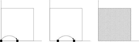
Figure 5: Position of a single $O(1)$ instanton: This $E1$ wraps the third $T^{2}$ and is localised on the fixed points $(x_{1},y_{1})=(0,0)+(1/2,0)$, $(x_{2},y_{2})=(1/4,0)+(3/4,0)$ of $\Theta$ .

Therefore, altogether we found $3\cdot 3\cdot 4=36$ $O(1)$ instantons which have the right zero mode structure to yield a single instanton correction to the gauge kinetic function of the pure $SO(32)$ super Yang-Mills theory on the $D9$-branes. For reasons that will become clear later, let us denote these instantons by

$$E1^{i,k}_{2},\quad E1^{i,k}_{3},\quad E1^{i,k}_{4}$$ (3.28)

with $i=1,2,3$ denoting the $T^{2}$ factor wrapped by the instanton, $k=1,2,3,4$ denoting the pair of fixed points where the instanton is located on the two remaining $T^{2}$ factors and finally the lower index denoting the discrete Wilson line turned on along $T^{2}_{i}$ with $E1_{2}=E1_{(0,{\textstyle{1\over 2}})},E1_{4}=E1_{(1,0)},E1_{3}=E1_{(1,{\textstyle{1\over 2}})}$.

3.3 The one-instanton sector

According to the formula (2.3) we now have to compute various gauge threshold corrections, which can be done quite analogously to the computation of N=2 sector gauge thresholds described in [37, 38, 39, 40].

First we have to compute the one-loop fluctuations around the $E1$ instantons, which are related to the threshold corrections and . In the amplitude for, say, the $D5$ brane shown in figure 5 only the $(1+\Theta)/2$ insertions in the trace give a non-vanishing contribution, as $\Theta^{\prime}$ and $\Theta^{\prime\prime}$ act by shifting the $D5$ along the first two $T^{2}$s. Denoting the Wilson lines along $D5$ as $(\alpha,\beta)$ and transforming the expression into tree-channel we get the general threshold corrections for this ${N}=2$ sector

$$\psset{unit=5.5pt,linewidth=0.25pt}\begin{pspicture}[0.5](0.0pt,0.0pt)(35.75pt,22.0pt){\psellipse(8.25pt,13.75pt)(5.5pt,8.25pt)}{\psellipse(27.5pt,13.75pt)(5.5pt,8.25pt)}{\psline{-}(8.25pt,22.0pt)(27.5pt,22.0pt)}{\psline{-}(8.25pt,5.5pt)(27.5pt,5.5pt)}\rput(8.25pt,1.375pt){$\scriptstyle D5$}\rput(27.5pt,1.375pt){$\scriptstyle D9$}\psset{linewidth=0.5pt}{\psline{-}(4.18pt,19.25pt)(5.82999pt,20.9pt)}{\psline{-}(4.18pt,19.25pt)(2.53pt,17.59999pt)}{\psline{-}(4.18pt,19.25pt)(5.82999pt,17.59999pt)}{\psline{-}(4.18pt,19.25pt)(2.53pt,20.9pt)}{\psline{-}(12.31999pt,8.25pt)(13.96999pt,9.9pt)}{\psline{-}(12.31999pt,8.25pt)(10.67pt,6.59999pt)}{\psline{-}(12.31999pt,8.25pt)(13.96999pt,6.59999pt)}{\psline{-}(12.31999pt,8.25pt)(10.67pt,9.9pt)}\end{pspicture}\,=\,\Re\left[\psset{unit=5.5pt,linewidth=0.25pt}\begin{pspicture}[0.5](0.0pt,0.0pt)(35.75pt,22.0pt){\psellipse(8.25pt,13.75pt)(5.5pt,8.25pt)}{\psellipse(27.5pt,13.75pt)(5.5pt,8.25pt)}{\psline{-}(8.25pt,22.0pt)(27.5pt,22.0pt)}{\psline{-}(8.25pt,5.5pt)(27.5pt,5.5pt)}\rput(8.25pt,1.375pt){$\scriptstyle E1$}\rput(27.5pt,1.375pt){$\scriptstyle D9$}\end{pspicture}\right]\, = 4\,\mathcal{T}_{2}\int_{0}^{\infty}dl\ \sum_{{r,s=-\infty\atop(r,s)\neq(0,0)}}^{\infty}e^{-{\pi\,\mathcal{T}_{2}\,l\over\mathcal{U}_{2}}\left|r+\mathcal{U}s\right|^{2}}\,e^{2\pi i(\alpha\,r+\beta\,s)}+$$

$$+4\,\mathcal{T}_{2}\int_{0}^{\infty}dl\ \sum_{r,s=-\infty}^{\infty}e^{-{\pi\,\mathcal{T}_{2}\,l\over\mathcal{U}_{2}}\left|r+{1\over 2}+\mathcal{U}s\right|^{2}}\,e^{2\pi i(\alpha\,(r+{1\over 2})+\beta\,s)}\;.$$

The appearing integrals are straightforward to compute using the methods from [37, 39, 40].

The threshold corrections arising from the Möbius strip amplitude only receive contributions from the undressed $\Omega$ insertion in the trace, as again $\Omega\Theta^{\prime}$ and $\Omega\Theta^{\prime\prime}$ shift the position of the $D5$-brane while $\Omega\Theta$ is an ${N}=4$ sector and therefore its threshold corrections vanish. It only remains to compute the integral

$$\psset{unit=5.5pt,linewidth=0.25pt}\begin{pspicture}[0.5](0.0pt,0.0pt)(35.75pt,22.0pt){\psellipse(8.25pt,13.75pt)(5.5pt,8.25pt)}{\psellipse(27.5pt,13.75pt)(5.5pt,8.25pt)}{\psline{-}(8.25pt,22.0pt)(27.5pt,22.0pt)}{\psline{-}(8.25pt,5.5pt)(27.5pt,5.5pt)}\rput(8.25pt,1.375pt){$\scriptstyle D5$}\rput(27.5pt,1.375pt){$\scriptstyle O9$}{\psline{-}(27.5pt,13.75pt)(23.43pt,19.25pt)}{\psline{-}(27.5pt,13.75pt)(31.56999pt,19.25pt)}{\psline{-}(27.5pt,13.75pt)(23.43pt,8.25pt)}{\psline{-}(27.5pt,13.75pt)(31.56999pt,8.25pt)}\psset{linewidth=0.5pt}{\psline{-}(4.18pt,19.25pt)(5.82999pt,20.9pt)}{\psline{-}(4.18pt,19.25pt)(2.53pt,17.59999pt)}{\psline{-}(4.18pt,19.25pt)(5.82999pt,17.59999pt)}{\psline{-}(4.18pt,19.25pt)(2.53pt,20.9pt)}{\psline{-}(12.31999pt,8.25pt)(13.96999pt,9.9pt)}{\psline{-}(12.31999pt,8.25pt)(10.67pt,6.59999pt)}{\psline{-}(12.31999pt,8.25pt)(13.96999pt,6.59999pt)}{\psline{-}(12.31999pt,8.25pt)(10.67pt,9.9pt)}\end{pspicture}\,=\,\Re\left[\psset{unit=5.5pt,linewidth=0.25pt}\begin{pspicture}[0.5](0.0pt,0.0pt)(35.75pt,22.0pt){\psellipse(8.25pt,13.75pt)(5.5pt,8.25pt)}{\psellipse(27.5pt,13.75pt)(5.5pt,8.25pt)}{\psline{-}(8.25pt,22.0pt)(27.5pt,22.0pt)}{\psline{-}(8.25pt,5.5pt)(27.5pt,5.5pt)}\rput(8.25pt,1.375pt){$\scriptstyle E1$}\rput(27.5pt,1.375pt){$\scriptstyle O9$}{\psline{-}(27.5pt,13.75pt)(23.43pt,19.25pt)}{\psline{-}(27.5pt,13.75pt)(31.56999pt,19.25pt)}{\psline{-}(27.5pt,13.75pt)(23.43pt,8.25pt)}{\psline{-}(27.5pt,13.75pt)(31.56999pt,8.25pt)}\end{pspicture}\right]\, = \mathcal{T}_{2}\int_{0}^{\infty}dl\ \sum_{{r,s=-\infty\atop(r,s)\neq(0,0)}}^{\infty}e^{-{\pi\,\mathcal{T}_{2}\,l\over\mathcal{U}_{2}}|r+\mathcal{U}s|^{2}}\;.$$ (3.30)

For an instanton $E1^{i,k}_{2,3,4}$ all these amplitudes do not depend on $k$ and on $i$ only via the changed argument $\mathcal{U}=\mathcal{U}_{i}$, while the functional form does depend on the discrete Wilson line. For the three types of discrete Wilson lines we obtain:

$\bullet\ E1_{2}$

For the $E1$-$D9$ annulus diagram we get

$$\psset{unit=5.5pt,linewidth=0.25pt}\begin{pspicture}[0.5](0.0pt,0.0pt)(35.75pt,22.0pt){\psellipse(8.25pt,13.75pt)(5.5pt,8.25pt)}{\psellipse(27.5pt,13.75pt)(5.5pt,8.25pt)}{\psline{-}(8.25pt,22.0pt)(27.5pt,22.0pt)}{\psline{-}(8.25pt,5.5pt)(27.5pt,5.5pt)}\rput(8.25pt,1.375pt){$\scriptstyle E1_{2}$}\rput(27.5pt,1.375pt){$\scriptstyle D9$}\end{pspicture}=-16\,\log\left({\vartheta_{2}\over\eta}(2\mathcal{U})\right)$$ (3.31)

where the prefactor of $16$ originates from the 32 $D9$-branes and for the Möbius strip we get the simple result

$$\psset{unit=5.5pt,linewidth=0.25pt}\begin{pspicture}[0.5](0.0pt,0.0pt)(35.75pt,22.0pt){\psellipse(8.25pt,13.75pt)(5.5pt,8.25pt)}{\psellipse(27.5pt,13.75pt)(5.5pt,8.25pt)}{\psline{-}(8.25pt,22.0pt)(27.5pt,22.0pt)}{\psline{-}(8.25pt,5.5pt)(27.5pt,5.5pt)}\rput(8.25pt,1.375pt){$\scriptstyle E1_{2}$}\rput(27.5pt,1.375pt){$\scriptstyle O9$}{\psline{-}(27.5pt,13.75pt)(23.43pt,19.25pt)}{\psline{-}(27.5pt,13.75pt)(31.56999pt,19.25pt)}{\psline{-}(27.5pt,13.75pt)(23.43pt,8.25pt)}{\psline{-}(27.5pt,13.75pt)(31.56999pt,8.25pt)}\end{pspicture}=4\,\log\left(\eta(\mathcal{U})\right)\;.$$ (3.32)

$\bullet\ E1_{3}$

For this instanton the computation of the $E1$-$D9$ annulus is up to one overall sign in front of the second term in (3.3) identical to the former case and we get

$$\psset{unit=5.5pt,linewidth=0.25pt}\begin{pspicture}[0.5](0.0pt,0.0pt)(35.75pt,22.0pt){\psellipse(8.25pt,13.75pt)(5.5pt,8.25pt)}{\psellipse(27.5pt,13.75pt)(5.5pt,8.25pt)}{\psline{-}(8.25pt,22.0pt)(27.5pt,22.0pt)}{\psline{-}(8.25pt,5.5pt)(27.5pt,5.5pt)}\rput(8.25pt,1.375pt){$\scriptstyle E1_{3}$}\rput(27.5pt,1.375pt){$\scriptstyle D9$}\end{pspicture}=-16\,\log\left({\vartheta_{3}\over\eta}(2\mathcal{U})\right)\;.$$ (3.33)

For the Möbius strip we get the same result as for the $E1_{2}$ instanton.

$\bullet\ E1_{4}$

Here the annulus diagram yields

$$\psset{unit=5.5pt,linewidth=0.25pt}\begin{pspicture}[0.5](0.0pt,0.0pt)(35.75pt,22.0pt){\psellipse(8.25pt,13.75pt)(5.5pt,8.25pt)}{\psellipse(27.5pt,13.75pt)(5.5pt,8.25pt)}{\psline{-}(8.25pt,22.0pt)(27.5pt,22.0pt)}{\psline{-}(8.25pt,5.5pt)(27.5pt,5.5pt)}\rput(8.25pt,1.375pt){$\scriptstyle E1_{4}$}\rput(27.5pt,1.375pt){$\scriptstyle D9$}\end{pspicture}=-16\,\log\left({\vartheta_{4}\over\eta}(2\mathcal{U})\right)$$ (3.34)

and again the Möbius strip amplitude is not changed.

Comparing this with the heterotic single instanton contribution in (3.17)-(3.17), we realise that the sum there corresponds to the three different classes of $E1$ instantons and that the Type I one-loop determinants  $\exp\bigl{[}-\psset{unit=3.5pt,linewidth=0.25pt}\begin{pspicture}[0.35](0.0pt,-1.75pt)(22.75pt,14.0pt){\psellipse(5.25pt,8.75pt)(3.5pt,5.25pt)}{\psellipse(17.5pt,8.75pt)(3.5pt,5.25pt)}{\psline{-}(5.25pt,14.0pt)(17.5pt,14.0pt)}{\psline{-}(5.25pt,3.5pt)(17.5pt,3.5pt)}\rput(5.25pt,0.875pt){$\scriptscriptstyle E1$}\rput(17.5pt,0.875pt){$\scriptscriptstyle D9$}\end{pspicture}-\psset{unit=3.5pt,linewidth=0.25pt}\begin{pspicture}[0.35](0.0pt,-1.75pt)(22.75pt,14.0pt){\psellipse(5.25pt,8.75pt)(3.5pt,5.25pt)}{\psellipse(17.5pt,8.75pt)(3.5pt,5.25pt)}{\psline{-}(5.25pt,14.0pt)(17.5pt,14.0pt)}{\psline{-}(5.25pt,3.5pt)(17.5pt,3.5pt)}\rput(5.25pt,0.875pt){$\scriptscriptstyle E1$}\rput(17.5pt,0.875pt){$\scriptscriptstyle O9$}{\psline{-}(17.5pt,8.75pt)(14.90999pt,12.25pt)}{\psline{-}(17.5pt,8.75pt)(20.09pt,12.25pt)}{\psline{-}(17.5pt,8.75pt)(14.90999pt,5.25pt)}{\psline{-}(17.5pt,8.75pt)(20.09pt,5.25pt)}\end{pspicture}\bigr{]}$  precisely give the first two factors in each line. It remains to compute the zero mode absorption annulus diagrams for the three types of $E1$-instantons. Recall from section 2.2 that these amplitudes are related to second derivatives of threshold corrections ${\partial^{2}\over\partial m^{2}}\psset{unit=3.5pt,linewidth=0.25pt}\begin{pspicture}[0.35](0.0pt,-1.75pt)(22.75pt,14.0pt){\psellipse(5.25pt,8.75pt)(3.5pt,5.25pt)}{\psellipse(17.5pt,8.75pt)(3.5pt,5.25pt)}{\psline{-}(5.25pt,14.0pt)(17.5pt,14.0pt)}{\psline{-}(5.25pt,3.5pt)(17.5pt,3.5pt)}\rput(5.25pt,0.875pt){$\scriptscriptstyle D5$}\rput(17.5pt,0.875pt){$\scriptscriptstyle D9$}\psset{linewidth=0.5pt}{\psline{-}(2.65999pt,12.25pt)(3.70999pt,13.29999pt)}{\psline{-}(2.65999pt,12.25pt)(1.60999pt,11.2pt)}{\psline{-}(2.65999pt,12.25pt)(3.70999pt,11.2pt)}{\psline{-}(2.65999pt,12.25pt)(1.60999pt,13.29999pt)}{\psline{-}(7.84pt,5.25pt)(8.89pt,6.29999pt)}{\psline{-}(7.84pt,5.25pt)(6.79pt,4.2pt)}{\psline{-}(7.84pt,5.25pt)(8.89pt,4.2pt)}{\psline{-}(7.84pt,5.25pt)(6.79pt,6.29999pt)}\end{pspicture}$. We have just computed the latter. Upon including a relative (continuous) Wilson line $m$ they take the form

$$\psset{unit=5.5pt,linewidth=0.25pt}\begin{pspicture}[0.5](0.0pt,0.0pt)(35.75pt,22.0pt){\psellipse(8.25pt,13.75pt)(5.5pt,8.25pt)}{\psellipse(27.5pt,13.75pt)(5.5pt,8.25pt)}{\psline{-}(8.25pt,22.0pt)(27.5pt,22.0pt)}{\psline{-}(8.25pt,5.5pt)(27.5pt,5.5pt)}\rput(8.25pt,1.375pt){$\scriptstyle D5_{r}$}\rput(27.5pt,1.375pt){$\scriptstyle D9$}\psset{linewidth=0.5pt}{\psline{-}(4.18pt,19.25pt)(5.82999pt,20.9pt)}{\psline{-}(4.18pt,19.25pt)(2.53pt,17.59999pt)}{\psline{-}(4.18pt,19.25pt)(5.82999pt,17.59999pt)}{\psline{-}(4.18pt,19.25pt)(2.53pt,20.9pt)}{\psline{-}(12.31999pt,8.25pt)(13.96999pt,9.9pt)}{\psline{-}(12.31999pt,8.25pt)(10.67pt,6.59999pt)}{\psline{-}(12.31999pt,8.25pt)(13.96999pt,6.59999pt)}{\psline{-}(12.31999pt,8.25pt)(10.67pt,9.9pt)}\end{pspicture}=-16\,\log\left({\vartheta_{r}(m,2\mathcal{U})\over\eta(2\mathcal{U})}\right)$$ (3.35)

for $r=2,3,4$. Therefore, for the three different classes of single $E1$ instantons, we get

$$\int d^{2}\theta\,d^{2}\mu\ \psset{unit=5.5pt,linewidth=0.25pt}\begin{pspicture}[0.5](0.0pt,0.0pt)(35.75pt,22.0pt){\psellipse(8.25pt,13.75pt)(5.5pt,8.25pt)}{\psellipse(27.5pt,13.75pt)(5.5pt,8.25pt)}{\psline{-}(8.25pt,22.0pt)(27.5pt,22.0pt)}{\psline{-}(8.25pt,5.5pt)(27.5pt,5.5pt)}\rput(8.25pt,1.375pt){$\scriptstyle D9$}\rput(27.5pt,1.375pt){$\scriptstyle E1_{2}$}\psset{linewidth=0.5pt}{\psline{-}(4.18pt,19.25pt)(5.82999pt,20.9pt)}{\psline{-}(4.18pt,19.25pt)(2.53pt,17.59999pt)}{\psline{-}(4.18pt,19.25pt)(5.82999pt,17.59999pt)}{\psline{-}(4.18pt,19.25pt)(2.53pt,20.9pt)}{\psline{-}(12.31999pt,8.25pt)(13.96999pt,9.9pt)}{\psline{-}(12.31999pt,8.25pt)(10.67pt,6.59999pt)}{\psline{-}(12.31999pt,8.25pt)(13.96999pt,6.59999pt)}{\psline{-}(12.31999pt,8.25pt)(10.67pt,9.9pt)}{\psline{-}(23.43pt,19.25pt)(25.07999pt,20.9pt)}{\psline{-}(23.43pt,19.25pt)(21.78pt,17.59999pt)}{\psline{-}(23.43pt,19.25pt)(25.07999pt,17.59999pt)}{\psline{-}(23.43pt,19.25pt)(21.78pt,20.9pt)}{\psline{-}(31.56999pt,19.25pt)(33.21999pt,20.9pt)}{\psline{-}(31.56999pt,19.25pt)(29.92pt,17.59999pt)}{\psline{-}(31.56999pt,19.25pt)(33.21999pt,17.59999pt)}{\psline{-}(31.56999pt,19.25pt)(29.92pt,20.9pt)}{\psline{-}(23.43pt,8.25pt)(25.07999pt,9.9pt)}{\psline{-}(23.43pt,8.25pt)(21.78pt,6.59999pt)}{\psline{-}(23.43pt,8.25pt)(25.07999pt,6.59999pt)}{\psline{-}(23.43pt,8.25pt)(21.78pt,9.9pt)}{\psline{-}(31.56999pt,8.25pt)(33.21999pt,9.9pt)}{\psline{-}(31.56999pt,8.25pt)(29.92pt,6.59999pt)}{\psline{-}(31.56999pt,8.25pt)(33.21999pt,6.59999pt)}{\psline{-}(31.56999pt,8.25pt)(29.92pt,9.9pt)}\end{pspicture}\,\simeq\,{\vartheta_{2}^{\prime\prime}\over\vartheta_{2}}(2\mathcal{U})=-{\pi^{2}\over 3}\left(E_{2}+\vartheta_{3}^{4}+\vartheta_{4}^{4}\right)(2\mathcal{U})$$

$$\int d^{2}\theta\,d^{2}\mu\ \psset{unit=5.5pt,linewidth=0.25pt}\begin{pspicture}[0.5](0.0pt,0.0pt)(35.75pt,22.0pt){\psellipse(8.25pt,13.75pt)(5.5pt,8.25pt)}{\psellipse(27.5pt,13.75pt)(5.5pt,8.25pt)}{\psline{-}(8.25pt,22.0pt)(27.5pt,22.0pt)}{\psline{-}(8.25pt,5.5pt)(27.5pt,5.5pt)}\rput(8.25pt,1.375pt){$\scriptstyle D9$}\rput(27.5pt,1.375pt){$\scriptstyle E1_{3}$}\psset{linewidth=0.5pt}{\psline{-}(4.18pt,19.25pt)(5.82999pt,20.9pt)}{\psline{-}(4.18pt,19.25pt)(2.53pt,17.59999pt)}{\psline{-}(4.18pt,19.25pt)(5.82999pt,17.59999pt)}{\psline{-}(4.18pt,19.25pt)(2.53pt,20.9pt)}{\psline{-}(12.31999pt,8.25pt)(13.96999pt,9.9pt)}{\psline{-}(12.31999pt,8.25pt)(10.67pt,6.59999pt)}{\psline{-}(12.31999pt,8.25pt)(13.96999pt,6.59999pt)}{\psline{-}(12.31999pt,8.25pt)(10.67pt,9.9pt)}{\psline{-}(23.43pt,19.25pt)(25.07999pt,20.9pt)}{\psline{-}(23.43pt,19.25pt)(21.78pt,17.59999pt)}{\psline{-}(23.43pt,19.25pt)(25.07999pt,17.59999pt)}{\psline{-}(23.43pt,19.25pt)(21.78pt,20.9pt)}{\psline{-}(31.56999pt,19.25pt)(33.21999pt,20.9pt)}{\psline{-}(31.56999pt,19.25pt)(29.92pt,17.59999pt)}{\psline{-}(31.56999pt,19.25pt)(33.21999pt,17.59999pt)}{\psline{-}(31.56999pt,19.25pt)(29.92pt,20.9pt)}{\psline{-}(23.43pt,8.25pt)(25.07999pt,9.9pt)}{\psline{-}(23.43pt,8.25pt)(21.78pt,6.59999pt)}{\psline{-}(23.43pt,8.25pt)(25.07999pt,6.59999pt)}{\psline{-}(23.43pt,8.25pt)(21.78pt,9.9pt)}{\psline{-}(31.56999pt,8.25pt)(33.21999pt,9.9pt)}{\psline{-}(31.56999pt,8.25pt)(29.92pt,6.59999pt)}{\psline{-}(31.56999pt,8.25pt)(33.21999pt,6.59999pt)}{\psline{-}(31.56999pt,8.25pt)(29.92pt,9.9pt)}\end{pspicture}\,\simeq\,{\vartheta_{3}^{\prime\prime}\over\vartheta_{3}}(2\mathcal{U})=-{\pi^{2}\over 3}\left(E_{2}+\vartheta_{2}^{4}-\vartheta_{4}^{4}\right)(2\mathcal{U})$$ (3.36)

$$\int d^{2}\theta\,d^{2}\mu\ \psset{unit=5.5pt,linewidth=0.25pt}\begin{pspicture}[0.5](0.0pt,0.0pt)(35.75pt,22.0pt){\psellipse(8.25pt,13.75pt)(5.5pt,8.25pt)}{\psellipse(27.5pt,13.75pt)(5.5pt,8.25pt)}{\psline{-}(8.25pt,22.0pt)(27.5pt,22.0pt)}{\psline{-}(8.25pt,5.5pt)(27.5pt,5.5pt)}\rput(8.25pt,1.375pt){$\scriptstyle D9$}\rput(27.5pt,1.375pt){$\scriptstyle E1_{4}$}\psset{linewidth=0.5pt}{\psline{-}(4.18pt,19.25pt)(5.82999pt,20.9pt)}{\psline{-}(4.18pt,19.25pt)(2.53pt,17.59999pt)}{\psline{-}(4.18pt,19.25pt)(5.82999pt,17.59999pt)}{\psline{-}(4.18pt,19.25pt)(2.53pt,20.9pt)}{\psline{-}(12.31999pt,8.25pt)(13.96999pt,9.9pt)}{\psline{-}(12.31999pt,8.25pt)(10.67pt,6.59999pt)}{\psline{-}(12.31999pt,8.25pt)(13.96999pt,6.59999pt)}{\psline{-}(12.31999pt,8.25pt)(10.67pt,9.9pt)}{\psline{-}(23.43pt,19.25pt)(25.07999pt,20.9pt)}{\psline{-}(23.43pt,19.25pt)(21.78pt,17.59999pt)}{\psline{-}(23.43pt,19.25pt)(25.07999pt,17.59999pt)}{\psline{-}(23.43pt,19.25pt)(21.78pt,20.9pt)}{\psline{-}(31.56999pt,19.25pt)(33.21999pt,20.9pt)}{\psline{-}(31.56999pt,19.25pt)(29.92pt,17.59999pt)}{\psline{-}(31.56999pt,19.25pt)(33.21999pt,17.59999pt)}{\psline{-}(31.56999pt,19.25pt)(29.92pt,20.9pt)}{\psline{-}(23.43pt,8.25pt)(25.07999pt,9.9pt)}{\psline{-}(23.43pt,8.25pt)(21.78pt,6.59999pt)}{\psline{-}(23.43pt,8.25pt)(25.07999pt,6.59999pt)}{\psline{-}(23.43pt,8.25pt)(21.78pt,9.9pt)}{\psline{-}(31.56999pt,8.25pt)(33.21999pt,9.9pt)}{\psline{-}(31.56999pt,8.25pt)(29.92pt,6.59999pt)}{\psline{-}(31.56999pt,8.25pt)(33.21999pt,6.59999pt)}{\psline{-}(31.56999pt,8.25pt)(29.92pt,9.9pt)}\end{pspicture}\,\simeq\,{\vartheta_{4}^{\prime\prime}\over\vartheta_{4}}(2\mathcal{U})=-{\pi^{2}\over 3}\left(E_{2}-\vartheta_{2}^{4}-\vartheta_{3}^{4}\right)(2\mathcal{U})\,,$$

which agree precisely with the third factor in each of the three heterotic contributions in (3.17)-(3.17).

We conclude that we managed to quantitatively match the holomorphic part of the single instanton contributions from the heterotic and the Type I side. We consider this as evidence that the (single) D-brane instanton calculus is correct and that in particular our formulas (2.15, 2.16) relating the four fermionic zero mode absorption annulus diagrams to second derivatives of gauge threshold corrections make sense. Both on the heterotic and the Type I side there are non-holomorphic corrections in the string diagrams, arising as effects of the massless modes. It would be interesting to see whether the instanton calculus on both sides gives complete agreement also for the entire string expressions and not just for their holomorphic Wilsonian pieces.

From the Type I perspective it is clear that the three contributions in (3.17)-(3.17) originate from three different $O(1)$ instantons distinguished by relative discrete Wilson lines. However, on the heterotic side the S-dual interpretation might not be so familiar, as the three terms are related to the GSO projection of the $32$ left-moving world-sheet fermions. However, it was already observed in [46] that the heterotic world-sheets with the four-different spin structures of the $32$ free fermions are related to the four possible $\mathbb{Z}_{2}$ Wilson-lines for the $O(1)$ D1-instantons. Indeed the fermions with PP-spin-structure do have zero modes, so that they do not contribute in (3.17)-(3.17) leaving only the three contributions AA, AP, PA.

3.4 Multiply wrapped single instantons

Having identified the single instanton contributions, it remains to clarify what the Type I S-dual of all the higher terms in the heterotic instanton expansion is. Very similar expressions have already appeared for other heterotic instanton corrections (see [44, 47, 45]), where it was pointed out that the higher terms are S-dual to certain bound states of $E1$-instantons, which can also be considered as single but multiply wrapped $E1$-instantons [48, 49].

In order to determine the contributions of these multiply wrapped instantons to the gauge kinetic function, one has to compute annulus and Möbius diagrams. They only differ from those appearing in the first order instanton sector in that the momentum/winding sums are changed. The necessary modification of these sums is most easily described by introducing the effective complex structure modulus $\mathcal{U}^{eff}$, which is just the complex structure modulus of the cycle the instanton wraps. This cycle covers one of the three two-tori that constitute the internal manifold several times. In other words, the lattice that defines the two-torus of the compactification manifold is a sublattice of the lattice that describes the cycle the instanton wraps. This is illustrated in figure 6. The equation (3.6) suggests that the effective complex structure modulus of the cycle wrapped by the instanton that captures the contribution corresponding to a particular matrix $A$ in the heterotic picture is encoded in

$$\left(\begin{matrix}1\,,\,\mathcal{U}\end{matrix}\right)A=\left(\begin{matrix}A_{11}+A_{21}\mathcal{U}\,,\,A_{12}+A_{22}\mathcal{U}\end{matrix}\right),$$ (3.37)

where $\mathcal{U}$ is the complex structure modulus of the torus the instanton wraps several times. More precisely, $\mathcal{U}^{eff}=(A_{12}+A_{22}\mathcal{U})/2(A_{11}+A_{21}\mathcal{U})$. Furthermore, it turns out that, in order to get a matching of the heterotic and type I results, one has to modularly transform the matrix $A$ such that $A_{11}\in\mathbb{Z}+1/2$ and $A_{12}\in\mathbb{Z}$.

The matrices of interest for the present case are given in (3.9) and we will now discuss the three cases distinguished by whether $k$ and $j$ are integer or half-integer. If $k\in\mathbb{Z}+1/2$ and $j\in\mathbb{Z}$ the matrix already has the correct structure and the effective complex structure modulus is given by $\mathcal{U}^{eff}=(j+p\mathcal{U})/2k$. The cycle the instantons wraps in this case is shown in figure 6. The annulus and Möbius diagrams are those that appear in the one-instanton sector with $\mathcal{U}$ replaced by $\mathcal{U}^{eff}$. One therefore finally finds that the instanton yields the contribution (3.12) to the heterotic amplitude.

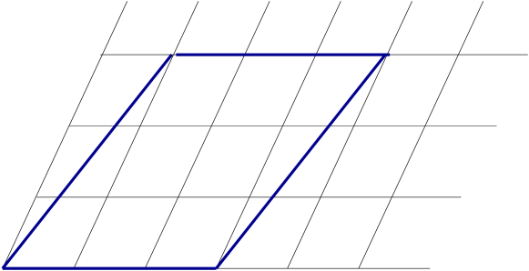
Figure 6: Multiply wrapped $E1$ instanton for $k\in\mathbb{Z}+{1\over 2}$ and $j,p\in\mathbb{Z}$.

If both $k$ and $j$ are half integers, one performs a modular T^-1 transformation on $A$ and obtains $\mathcal{U}^{eff}=(j-k+p\mathcal{U})/2k$. As in the previous case, the annulus and Möbius diagrams are those of the one-instanton amplitudes, so one finds the one-instanton result with $\mathcal{U}$ replaced by $\mathcal{U}^{eff}=(j-k+p\mathcal{U})/k$, i.e. (3.12) with argument$(j-k+p\mathcal{U})/k$. Applying a modular T transformation this can be rewritten and reproduces the term (3.13) in the heterotic amplitude.

Finally, if $k\in\mathbb{Z}$ and $j\in\mathbb{Z}+1/2$ one finds, after a modular S transformation on $A$, $\mathcal{U}^{eff}=-k/2(j+p\mathcal{U})$. Another modular S transformation, this one on the full instanton amplitude, gives the required result, the third term (3.11) of the heterotic amplitude.

3.5 The two-instanton sector

Let us now look more closely at the second order instanton sector. The two heterotic orbits characterised by

$$A=\left(\begin{matrix}{1\over 2}&0\\ 0&2\end{matrix}\right),\quad\quad A=\left(\begin{matrix}1&{1\over 2}\\ 0&1\end{matrix}\right)\;$$ (3.38)

correspond to the twice-wrapped $E1$-instantons shown in figure 7.

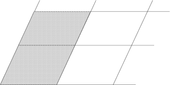
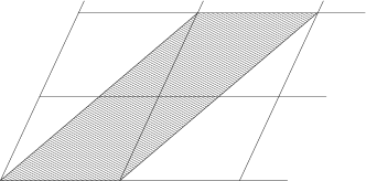
Figure 7: Left: $E1$ instanton for $k={1\over 2}$, $j=0$, $p=2$ . Right: $E1$ instanton for $k={1}$, $j={1\over 2}$, $p=1$

However, what about the various Type I poly two-instanton contributions

$$E1^{i,k}_{3}-E1^{i^{\prime},k^{\prime}}_{4},\quad\quad E1^{i,k}_{2}-E1^{i^{\prime},k^{\prime}}_{4}\quad\quad E1^{i,k}_{2}-E1^{i^{\prime},k^{\prime}}_{3}\;$$ (3.39)

which arise at the same second order in $\exp(2\pi i\mathcal{T})$ and which in section 2 we proposed to exist?

First, following our $E1$-instanton calculus introduced in section 2, let us compute these genuine two instanton contributions explicitly. We note that for $i\neq i^{\prime}$ the zero mode absorption amplitude vanishes, as the two instantons wrap different $T^{2}$s so that the threshold correction cannot depend on any of the Wilson-lines along the cycles of the two instantons. Similarly, for $i=i^{\prime}$ but $k\neq k^{\prime}$ the amplitude vanishes because there are no momentum modes invariant under the $\Theta$ insertion. Therefore, we only have to consider the case $i=i^{\prime}$ and $k=k^{\prime}$. For instance, the first amplitude (up to a normalisation factor $\kappa$) we expect to be equal to

$$\Lambda\left(E1_{3},E1_{4}\right) = \kappa\,\int d^{4}x_{rs}\,d^{2}\theta_{r}\,d^{2}\theta_{s}\,d^{2}\mu_{r}\,d^{2}\mu_{s}\ \left(\psset{unit=5.5pt,linewidth=0.25pt}\begin{pspicture}[0.5](0.0pt,0.0pt)(35.75pt,22.0pt){\psellipse(8.25pt,13.75pt)(5.5pt,8.25pt)}{\psellipse(27.5pt,13.75pt)(5.5pt,8.25pt)}{\psline{-}(8.25pt,22.0pt)(27.5pt,22.0pt)}{\psline{-}(8.25pt,5.5pt)(27.5pt,5.5pt)}\rput(8.25pt,1.375pt){$\scriptstyle D9$}\rput(27.5pt,1.375pt){$\scriptstyle E1_{3}$}\psset{linewidth=0.5pt}{\psline{-}(4.18pt,19.25pt)(5.82999pt,20.9pt)}{\psline{-}(4.18pt,19.25pt)(2.53pt,17.59999pt)}{\psline{-}(4.18pt,19.25pt)(5.82999pt,17.59999pt)}{\psline{-}(4.18pt,19.25pt)(2.53pt,20.9pt)}{\psline{-}(12.31999pt,8.25pt)(13.96999pt,9.9pt)}{\psline{-}(12.31999pt,8.25pt)(10.67pt,6.59999pt)}{\psline{-}(12.31999pt,8.25pt)(13.96999pt,6.59999pt)}{\psline{-}(12.31999pt,8.25pt)(10.67pt,9.9pt)}{\psline{-}(23.43pt,19.25pt)(25.07999pt,20.9pt)}{\psline{-}(23.43pt,19.25pt)(21.78pt,17.59999pt)}{\psline{-}(23.43pt,19.25pt)(25.07999pt,17.59999pt)}{\psline{-}(23.43pt,19.25pt)(21.78pt,20.9pt)}{\psline{-}(31.56999pt,19.25pt)(33.21999pt,20.9pt)}{\psline{-}(31.56999pt,19.25pt)(29.92pt,17.59999pt)}{\psline{-}(31.56999pt,19.25pt)(33.21999pt,17.59999pt)}{\psline{-}(31.56999pt,19.25pt)(29.92pt,20.9pt)}{\psline{-}(23.43pt,8.25pt)(25.07999pt,9.9pt)}{\psline{-}(23.43pt,8.25pt)(21.78pt,6.59999pt)}{\psline{-}(23.43pt,8.25pt)(25.07999pt,6.59999pt)}{\psline{-}(23.43pt,8.25pt)(21.78pt,9.9pt)}{\psline{-}(31.56999pt,8.25pt)(33.21999pt,9.9pt)}{\psline{-}(31.56999pt,8.25pt)(29.92pt,6.59999pt)}{\psline{-}(31.56999pt,8.25pt)(33.21999pt,6.59999pt)}{\psline{-}(31.56999pt,8.25pt)(29.92pt,9.9pt)}\end{pspicture}\,\psset{unit=5.5pt,linewidth=0.25pt}\begin{pspicture}[0.5](0.0pt,0.0pt)(35.75pt,22.0pt){\psellipse(8.25pt,13.75pt)(5.5pt,8.25pt)}{\psellipse(27.5pt,13.75pt)(5.5pt,8.25pt)}{\psline{-}(8.25pt,22.0pt)(27.5pt,22.0pt)}{\psline{-}(8.25pt,5.5pt)(27.5pt,5.5pt)}\rput(8.25pt,1.375pt){$\scriptstyle E1_{3}$}\rput(27.5pt,1.375pt){$\scriptstyle E1_{4}$}\psset{linewidth=0.5pt}{\psline{-}(23.43pt,19.25pt)(25.07999pt,20.9pt)}{\psline{-}(23.43pt,19.25pt)(21.78pt,17.59999pt)}{\psline{-}(23.43pt,19.25pt)(25.07999pt,17.59999pt)}{\psline{-}(23.43pt,19.25pt)(21.78pt,20.9pt)}{\psline{-}(31.56999pt,19.25pt)(33.21999pt,20.9pt)}{\psline{-}(31.56999pt,19.25pt)(29.92pt,17.59999pt)}{\psline{-}(31.56999pt,19.25pt)(33.21999pt,17.59999pt)}{\psline{-}(31.56999pt,19.25pt)(29.92pt,20.9pt)}{\psline{-}(23.43pt,8.25pt)(25.07999pt,9.9pt)}{\psline{-}(23.43pt,8.25pt)(21.78pt,6.59999pt)}{\psline{-}(23.43pt,8.25pt)(25.07999pt,6.59999pt)}{\psline{-}(23.43pt,8.25pt)(21.78pt,9.9pt)}{\psline{-}(31.56999pt,8.25pt)(33.21999pt,9.9pt)}{\psline{-}(31.56999pt,8.25pt)(29.92pt,6.59999pt)}{\psline{-}(31.56999pt,8.25pt)(33.21999pt,6.59999pt)}{\psline{-}(31.56999pt,8.25pt)(29.92pt,9.9pt)}\end{pspicture}+\psset{unit=5.5pt,linewidth=0.25pt}\begin{pspicture}[0.5](0.0pt,0.0pt)(35.75pt,22.0pt){\psellipse(8.25pt,13.75pt)(5.5pt,8.25pt)}{\psellipse(27.5pt,13.75pt)(5.5pt,8.25pt)}{\psline{-}(8.25pt,22.0pt)(27.5pt,22.0pt)}{\psline{-}(8.25pt,5.5pt)(27.5pt,5.5pt)}\rput(8.25pt,1.375pt){$\scriptstyle D9$}\rput(27.5pt,1.375pt){$\scriptstyle E1_{4}$}\psset{linewidth=0.5pt}{\psline{-}(4.18pt,19.25pt)(5.82999pt,20.9pt)}{\psline{-}(4.18pt,19.25pt)(2.53pt,17.59999pt)}{\psline{-}(4.18pt,19.25pt)(5.82999pt,17.59999pt)}{\psline{-}(4.18pt,19.25pt)(2.53pt,20.9pt)}{\psline{-}(12.31999pt,8.25pt)(13.96999pt,9.9pt)}{\psline{-}(12.31999pt,8.25pt)(10.67pt,6.59999pt)}{\psline{-}(12.31999pt,8.25pt)(13.96999pt,6.59999pt)}{\psline{-}(12.31999pt,8.25pt)(10.67pt,9.9pt)}{\psline{-}(23.43pt,19.25pt)(25.07999pt,20.9pt)}{\psline{-}(23.43pt,19.25pt)(21.78pt,17.59999pt)}{\psline{-}(23.43pt,19.25pt)(25.07999pt,17.59999pt)}{\psline{-}(23.43pt,19.25pt)(21.78pt,20.9pt)}{\psline{-}(31.56999pt,19.25pt)(33.21999pt,20.9pt)}{\psline{-}(31.56999pt,19.25pt)(29.92pt,17.59999pt)}{\psline{-}(31.56999pt,19.25pt)(33.21999pt,17.59999pt)}{\psline{-}(31.56999pt,19.25pt)(29.92pt,20.9pt)}{\psline{-}(23.43pt,8.25pt)(25.07999pt,9.9pt)}{\psline{-}(23.43pt,8.25pt)(21.78pt,6.59999pt)}{\psline{-}(23.43pt,8.25pt)(25.07999pt,6.59999pt)}{\psline{-}(23.43pt,8.25pt)(21.78pt,9.9pt)}{\psline{-}(31.56999pt,8.25pt)(33.21999pt,9.9pt)}{\psline{-}(31.56999pt,8.25pt)(29.92pt,6.59999pt)}{\psline{-}(31.56999pt,8.25pt)(33.21999pt,6.59999pt)}{\psline{-}(31.56999pt,8.25pt)(29.92pt,9.9pt)}\end{pspicture}\,\psset{unit=5.5pt,linewidth=0.25pt}\begin{pspicture}[0.5](0.0pt,0.0pt)(35.75pt,22.0pt){\psellipse(8.25pt,13.75pt)(5.5pt,8.25pt)}{\psellipse(27.5pt,13.75pt)(5.5pt,8.25pt)}{\psline{-}(8.25pt,22.0pt)(27.5pt,22.0pt)}{\psline{-}(8.25pt,5.5pt)(27.5pt,5.5pt)}\rput(8.25pt,1.375pt){$\scriptstyle E1_{4}$}\rput(27.5pt,1.375pt){$\scriptstyle E1_{3}$}\psset{linewidth=0.5pt}{\psline{-}(23.43pt,19.25pt)(25.07999pt,20.9pt)}{\psline{-}(23.43pt,19.25pt)(21.78pt,17.59999pt)}{\psline{-}(23.43pt,19.25pt)(25.07999pt,17.59999pt)}{\psline{-}(23.43pt,19.25pt)(21.78pt,20.9pt)}{\psline{-}(31.56999pt,19.25pt)(33.21999pt,20.9pt)}{\psline{-}(31.56999pt,19.25pt)(29.92pt,17.59999pt)}{\psline{-}(31.56999pt,19.25pt)(33.21999pt,17.59999pt)}{\psline{-}(31.56999pt,19.25pt)(29.92pt,20.9pt)}{\psline{-}(23.43pt,8.25pt)(25.07999pt,9.9pt)}{\psline{-}(23.43pt,8.25pt)(21.78pt,6.59999pt)}{\psline{-}(23.43pt,8.25pt)(25.07999pt,6.59999pt)}{\psline{-}(23.43pt,8.25pt)(21.78pt,9.9pt)}{\psline{-}(31.56999pt,8.25pt)(33.21999pt,9.9pt)}{\psline{-}(31.56999pt,8.25pt)(29.92pt,6.59999pt)}{\psline{-}(31.56999pt,8.25pt)(33.21999pt,6.59999pt)}{\psline{-}(31.56999pt,8.25pt)(29.92pt,9.9pt)}\end{pspicture}\right)$$ (3.40)

$$\exp\left(-\psset{unit=5.5pt,linewidth=0.25pt}\begin{pspicture}[0.5](0.0pt,0.0pt)(35.75pt,22.0pt){\psellipse(8.25pt,13.75pt)(5.5pt,8.25pt)}{\psellipse(27.5pt,13.75pt)(5.5pt,8.25pt)}{\psline{-}(8.25pt,22.0pt)(27.5pt,22.0pt)}{\psline{-}(8.25pt,5.5pt)(27.5pt,5.5pt)}\rput(8.25pt,1.375pt){$\scriptstyle E1_{3}$}\rput(27.5pt,1.375pt){$\scriptstyle D9$}\end{pspicture}-\psset{unit=5.5pt,linewidth=0.25pt}\begin{pspicture}[0.5](0.0pt,0.0pt)(35.75pt,22.0pt){\psellipse(8.25pt,13.75pt)(5.5pt,8.25pt)}{\psellipse(27.5pt,13.75pt)(5.5pt,8.25pt)}{\psline{-}(8.25pt,22.0pt)(27.5pt,22.0pt)}{\psline{-}(8.25pt,5.5pt)(27.5pt,5.5pt)}\rput(8.25pt,1.375pt){$\scriptstyle E1_{3}$}\rput(27.5pt,1.375pt){$\scriptstyle O9$}{\psline{-}(27.5pt,13.75pt)(23.43pt,19.25pt)}{\psline{-}(27.5pt,13.75pt)(31.56999pt,19.25pt)}{\psline{-}(27.5pt,13.75pt)(23.43pt,8.25pt)}{\psline{-}(27.5pt,13.75pt)(31.56999pt,8.25pt)}\end{pspicture}\!\right)\,\exp\left(-\psset{unit=5.5pt,linewidth=0.25pt}\begin{pspicture}[0.5](0.0pt,0.0pt)(35.75pt,22.0pt){\psellipse(8.25pt,13.75pt)(5.5pt,8.25pt)}{\psellipse(27.5pt,13.75pt)(5.5pt,8.25pt)}{\psline{-}(8.25pt,22.0pt)(27.5pt,22.0pt)}{\psline{-}(8.25pt,5.5pt)(27.5pt,5.5pt)}\rput(8.25pt,1.375pt){$\scriptstyle E1_{4}$}\rput(27.5pt,1.375pt){$\scriptstyle D9$}\end{pspicture}-\psset{unit=5.5pt,linewidth=0.25pt}\begin{pspicture}[0.5](0.0pt,0.0pt)(35.75pt,22.0pt){\psellipse(8.25pt,13.75pt)(5.5pt,8.25pt)}{\psellipse(27.5pt,13.75pt)(5.5pt,8.25pt)}{\psline{-}(8.25pt,22.0pt)(27.5pt,22.0pt)}{\psline{-}(8.25pt,5.5pt)(27.5pt,5.5pt)}\rput(8.25pt,1.375pt){$\scriptstyle E1_{4}$}\rput(27.5pt,1.375pt){$\scriptstyle O9$}{\psline{-}(27.5pt,13.75pt)(23.43pt,19.25pt)}{\psline{-}(27.5pt,13.75pt)(31.56999pt,19.25pt)}{\psline{-}(27.5pt,13.75pt)(23.43pt,8.25pt)}{\psline{-}(27.5pt,13.75pt)(31.56999pt,8.25pt)}\end{pspicture}\!\right)\ \,e^{2\pi i\,\mathcal{T}}$$

In order to determine $\psset{unit=3.5pt,linewidth=0.25pt}\begin{pspicture}[0.35](0.0pt,-1.75pt)(22.75pt,14.0pt){\psellipse(5.25pt,8.75pt)(3.5pt,5.25pt)}{\psellipse(17.5pt,8.75pt)(3.5pt,5.25pt)}{\psline{-}(5.25pt,14.0pt)(17.5pt,14.0pt)}{\psline{-}(5.25pt,3.5pt)(17.5pt,3.5pt)}\rput(5.25pt,0.875pt){$\scriptscriptstyle E1_{3}\,$}\rput(17.5pt,0.875pt){$\scriptscriptstyle\,E1_{4}$}\psset{linewidth=0.5pt}{\psline{-}(14.90999pt,12.25pt)(15.95999pt,13.29999pt)}{\psline{-}(14.90999pt,12.25pt)(13.85999pt,11.2pt)}{\psline{-}(14.90999pt,12.25pt)(15.95999pt,11.2pt)}{\psline{-}(14.90999pt,12.25pt)(13.85999pt,13.29999pt)}{\psline{-}(20.09pt,12.25pt)(21.14pt,13.29999pt)}{\psline{-}(20.09pt,12.25pt)(19.04pt,11.2pt)}{\psline{-}(20.09pt,12.25pt)(21.14pt,11.2pt)}{\psline{-}(20.09pt,12.25pt)(19.04pt,13.29999pt)}{\psline{-}(14.90999pt,5.25pt)(15.95999pt,6.29999pt)}{\psline{-}(14.90999pt,5.25pt)(13.85999pt,4.2pt)}{\psline{-}(14.90999pt,5.25pt)(15.95999pt,4.2pt)}{\psline{-}(14.90999pt,5.25pt)(13.85999pt,6.29999pt)}{\psline{-}(20.09pt,5.25pt)(21.14pt,6.29999pt)}{\psline{-}(20.09pt,5.25pt)(19.04pt,4.2pt)}{\psline{-}(20.09pt,5.25pt)(21.14pt,4.2pt)}{\psline{-}(20.09pt,5.25pt)(19.04pt,6.29999pt)}\end{pspicture}\hskip 3.0pt=\hskip 3.0pt\psset{unit=3.5pt,linewidth=0.25pt}\begin{pspicture}[0.35](0.0pt,-1.75pt)(22.75pt,14.0pt){\psellipse(5.25pt,8.75pt)(3.5pt,5.25pt)}{\psellipse(17.5pt,8.75pt)(3.5pt,5.25pt)}{\psline{-}(5.25pt,14.0pt)(17.5pt,14.0pt)}{\psline{-}(5.25pt,3.5pt)(17.5pt,3.5pt)}\rput(5.25pt,0.875pt){$\scriptscriptstyle E1_{4}\,$}\rput(17.5pt,0.875pt){$\scriptscriptstyle\,E1_{3}$}\psset{linewidth=0.5pt}{\psline{-}(14.90999pt,12.25pt)(15.95999pt,13.29999pt)}{\psline{-}(14.90999pt,12.25pt)(13.85999pt,11.2pt)}{\psline{-}(14.90999pt,12.25pt)(15.95999pt,11.2pt)}{\psline{-}(14.90999pt,12.25pt)(13.85999pt,13.29999pt)}{\psline{-}(20.09pt,12.25pt)(21.14pt,13.29999pt)}{\psline{-}(20.09pt,12.25pt)(19.04pt,11.2pt)}{\psline{-}(20.09pt,12.25pt)(21.14pt,11.2pt)}{\psline{-}(20.09pt,12.25pt)(19.04pt,13.29999pt)}{\psline{-}(14.90999pt,5.25pt)(15.95999pt,6.29999pt)}{\psline{-}(14.90999pt,5.25pt)(13.85999pt,4.2pt)}{\psline{-}(14.90999pt,5.25pt)(15.95999pt,4.2pt)}{\psline{-}(14.90999pt,5.25pt)(13.85999pt,6.29999pt)}{\psline{-}(20.09pt,5.25pt)(21.14pt,6.29999pt)}{\psline{-}(20.09pt,5.25pt)(19.04pt,4.2pt)}{\psline{-}(20.09pt,5.25pt)(21.14pt,4.2pt)}{\psline{-}(20.09pt,5.25pt)(19.04pt,6.29999pt)}\end{pspicture}\,$, we only have to compute the second derivative of . As the $E1_{3}$ and $E1_{4}$ instantonic branes are parallel on all three $T^{2}$s, only the term with the $\Theta$ insertion (in loop channel) contributes to the threshold correction amplitude , and we find

$$\psset{unit=5.5pt,linewidth=0.25pt}\begin{pspicture}[0.5](0.0pt,0.0pt)(35.75pt,22.0pt){\psellipse(8.25pt,13.75pt)(5.5pt,8.25pt)}{\psellipse(27.5pt,13.75pt)(5.5pt,8.25pt)}{\psline{-}(8.25pt,22.0pt)(27.5pt,22.0pt)}{\psline{-}(8.25pt,5.5pt)(27.5pt,5.5pt)}\rput(8.25pt,1.375pt){$\scriptstyle D5_{3}$}\rput(27.5pt,1.375pt){$\scriptstyle D5_{4}$}\psset{linewidth=0.5pt}{\psline{-}(23.43pt,19.25pt)(25.07999pt,20.9pt)}{\psline{-}(23.43pt,19.25pt)(21.78pt,17.59999pt)}{\psline{-}(23.43pt,19.25pt)(25.07999pt,17.59999pt)}{\psline{-}(23.43pt,19.25pt)(21.78pt,20.9pt)}{\psline{-}(31.56999pt,8.25pt)(33.21999pt,9.9pt)}{\psline{-}(31.56999pt,8.25pt)(29.92pt,6.59999pt)}{\psline{-}(31.56999pt,8.25pt)(33.21999pt,6.59999pt)}{\psline{-}(31.56999pt,8.25pt)(29.92pt,9.9pt)}\end{pspicture}=\log\left({\vartheta_{2}\over\vartheta_{3}}(2\mathcal{U})\right)$$ (3.41)

leading to

$$\int d^{4}x_{rs}\,\,d^{2}\theta_{s}\,d^{2}\mu_{s}\ \psset{unit=5.5pt,linewidth=0.25pt}\begin{pspicture}[0.5](0.0pt,0.0pt)(35.75pt,22.0pt){\psellipse(8.25pt,13.75pt)(5.5pt,8.25pt)}{\psellipse(27.5pt,13.75pt)(5.5pt,8.25pt)}{\psline{-}(8.25pt,22.0pt)(27.5pt,22.0pt)}{\psline{-}(8.25pt,5.5pt)(27.5pt,5.5pt)}\rput(8.25pt,1.375pt){$\scriptstyle E1_{3}$}\rput(27.5pt,1.375pt){$\scriptstyle E1_{4}$}\psset{linewidth=0.5pt}{\psline{-}(23.43pt,19.25pt)(25.07999pt,20.9pt)}{\psline{-}(23.43pt,19.25pt)(21.78pt,17.59999pt)}{\psline{-}(23.43pt,19.25pt)(25.07999pt,17.59999pt)}{\psline{-}(23.43pt,19.25pt)(21.78pt,20.9pt)}{\psline{-}(31.56999pt,19.25pt)(33.21999pt,20.9pt)}{\psline{-}(31.56999pt,19.25pt)(29.92pt,17.59999pt)}{\psline{-}(31.56999pt,19.25pt)(33.21999pt,17.59999pt)}{\psline{-}(31.56999pt,19.25pt)(29.92pt,20.9pt)}{\psline{-}(23.43pt,8.25pt)(25.07999pt,9.9pt)}{\psline{-}(23.43pt,8.25pt)(21.78pt,6.59999pt)}{\psline{-}(23.43pt,8.25pt)(25.07999pt,6.59999pt)}{\psline{-}(23.43pt,8.25pt)(21.78pt,9.9pt)}{\psline{-}(31.56999pt,8.25pt)(33.21999pt,9.9pt)}{\psline{-}(31.56999pt,8.25pt)(29.92pt,6.59999pt)}{\psline{-}(31.56999pt,8.25pt)(33.21999pt,6.59999pt)}{\psline{-}(31.56999pt,8.25pt)(29.92pt,9.9pt)}\end{pspicture}\simeq{\partial^{2}\over\partial m^{2}}\psset{unit=5.5pt,linewidth=0.25pt}\begin{pspicture}[0.5](0.0pt,0.0pt)(35.75pt,22.0pt){\psellipse(8.25pt,13.75pt)(5.5pt,8.25pt)}{\psellipse(27.5pt,13.75pt)(5.5pt,8.25pt)}{\psline{-}(8.25pt,22.0pt)(27.5pt,22.0pt)}{\psline{-}(8.25pt,5.5pt)(27.5pt,5.5pt)}\rput(8.25pt,1.375pt){$\scriptstyle D5_{3}$}\rput(27.5pt,1.375pt){$\scriptstyle D5_{4}$}\psset{linewidth=0.5pt}{\psline{-}(23.43pt,19.25pt)(25.07999pt,20.9pt)}{\psline{-}(23.43pt,19.25pt)(21.78pt,17.59999pt)}{\psline{-}(23.43pt,19.25pt)(25.07999pt,17.59999pt)}{\psline{-}(23.43pt,19.25pt)(21.78pt,20.9pt)}{\psline{-}(31.56999pt,8.25pt)(33.21999pt,9.9pt)}{\psline{-}(31.56999pt,8.25pt)(29.92pt,6.59999pt)}{\psline{-}(31.56999pt,8.25pt)(33.21999pt,6.59999pt)}{\psline{-}(31.56999pt,8.25pt)(29.92pt,9.9pt)}\end{pspicture}\biggr{|}_{m=0}\simeq{\vartheta^{\prime\prime}_{2}\over\vartheta_{2}}-{\vartheta^{\prime\prime}_{3}\over\vartheta_{3}}=-\pi^{2}\,\vartheta_{4}^{4}(2\mathcal{U})\;.$$ (3.42)

Collecting all terms, we find for this two instanton amplitude

$$\Lambda\left(E1_{3},E1_{4}\right)={\pi^{4}\kappa\over 3}\,e^{2\pi i\mathcal{T}}\ {\vartheta_{4}^{4}(2\mathcal{U})\over\eta^{8}(\mathcal{U})}\left({\vartheta_{3}\vartheta_{4}\over\eta^{2}}(2\mathcal{U})\right)^{\!\!16}\!(2\,E_{2}-\vartheta^{4}_{3}-\vartheta^{4}_{4})(2\mathcal{U})\;,\quad$$ (3.43)

which invoking some $\vartheta$-function identities can be written as

$$\Lambda\left(E1_{3},E1_{4}\right)={4\pi^{4}\kappa\over 3}\,{e^{2\pi i\,\mathcal{T}}\over\eta^{4}(2\mathcal{U})}\,\,\left({\vartheta_{4}\over\eta}(4\mathcal{U})\right)^{\!\!16}\left(E_{2}-\vartheta_{2}^{4}-\vartheta_{3}^{4}\right)(4\mathcal{U})\;.$$ (3.44)

One realises that this has precisely the form of the holomorphic part of the heterotic contribution (3.26), which naively could mean that this poly-instanton contribution is already included in the heterotic expression of multiply wrapped single instantons.

The other possibility is that the equality is more a coincidence in the sense that a D-brane wrapped twice around a cycle $b$ has (up a to normalisation factor two) the same partition function as a pair of singly wrapped D-branes with relative Wilson line $w={1\over 2}$ along the cycle $b$. This would explain why the two-instanton sector $E1_{3}-E1_{4}$ has the same functional form as the doubly wrapped one instanton $E1_{4}$. In this latter case, the fact that we really get the same result for the two-instanton and single doubly-wrapped instanton corrections establishes another positive test of the formulas (3.40) and (3.41).

Before we draw our final conclusions, let us proceed and collect more data. Completely analogously, using

$$\int d^{4}x_{rs}\,\,d^{2}\theta_{s}\,d^{2}\mu_{s}\ \psset{unit=5.5pt,linewidth=0.25pt}\begin{pspicture}[0.5](0.0pt,0.0pt)(35.75pt,22.0pt){\psellipse(8.25pt,13.75pt)(5.5pt,8.25pt)}{\psellipse(27.5pt,13.75pt)(5.5pt,8.25pt)}{\psline{-}(8.25pt,22.0pt)(27.5pt,22.0pt)}{\psline{-}(8.25pt,5.5pt)(27.5pt,5.5pt)}\rput(8.25pt,1.375pt){$\scriptstyle E1_{2}$}\rput(27.5pt,1.375pt){$\scriptstyle E1_{4}$}\psset{linewidth=0.5pt}{\psline{-}(23.43pt,19.25pt)(25.07999pt,20.9pt)}{\psline{-}(23.43pt,19.25pt)(21.78pt,17.59999pt)}{\psline{-}(23.43pt,19.25pt)(25.07999pt,17.59999pt)}{\psline{-}(23.43pt,19.25pt)(21.78pt,20.9pt)}{\psline{-}(31.56999pt,19.25pt)(33.21999pt,20.9pt)}{\psline{-}(31.56999pt,19.25pt)(29.92pt,17.59999pt)}{\psline{-}(31.56999pt,19.25pt)(33.21999pt,17.59999pt)}{\psline{-}(31.56999pt,19.25pt)(29.92pt,20.9pt)}{\psline{-}(23.43pt,8.25pt)(25.07999pt,9.9pt)}{\psline{-}(23.43pt,8.25pt)(21.78pt,6.59999pt)}{\psline{-}(23.43pt,8.25pt)(25.07999pt,6.59999pt)}{\psline{-}(23.43pt,8.25pt)(21.78pt,9.9pt)}{\psline{-}(31.56999pt,8.25pt)(33.21999pt,9.9pt)}{\psline{-}(31.56999pt,8.25pt)(29.92pt,6.59999pt)}{\psline{-}(31.56999pt,8.25pt)(33.21999pt,6.59999pt)}{\psline{-}(31.56999pt,8.25pt)(29.92pt,9.9pt)}\end{pspicture}\simeq\pi^{2}\,\vartheta_{4}^{4}(2\mathcal{U})\;$$ (3.45)

we can compute the $E1_{2}-E1_{4}$ poly-instanton correction and obtain

$$\Lambda\left(E1_{2},E1_{4}\right)=-{\pi^{4}\kappa\over 3}\,e^{2\pi i\mathcal{T}}\ {\vartheta_{4}^{4}(2\mathcal{U})\over\eta^{8}(\mathcal{U})}\left({\vartheta_{2}\vartheta_{4}\over\eta^{2}}(2\mathcal{U})\right)^{\!\!16}\!(2\,E_{2}-\vartheta^{4}_{2}+\vartheta^{4}_{4})(2\mathcal{U})\quad$$ (3.46)

which can be expressed as

$$\Lambda\left(E1_{2},E1_{4}\right)={\pi^{4}\kappa\over 3}\,e^{-\pi i/3}{e^{2\pi i\,\mathcal{T}}\over\eta^{4}(2\mathcal{U})}\,\,\left({\vartheta_{2}\over\eta}({\textstyle{1\over 2}}+\mathcal{U})\right)^{\!\!16}\left(E_{2}+\vartheta_{3}^{4}+\vartheta_{4}^{4}\right)({\textstyle{1\over 2}}+\mathcal{U})\;.$$

This expression is equal to the heterotic contribution (3.26) arising from the other orbit. These two singly wrapped instantons have the same partition function as the doubly wrapped single instanton $E1_{2}$. Note, that with the modular properties (3.19) it is obvious that under $U^{2}$ the two contributions (3.46) and (3.43) get exchanged.

It remains to discuss the $E1_{2}-E1_{3}$ poly-instanton correction. However, since these two instantons are only different by a relative Wilson line $(\alpha,\beta)=(1,0)$, there appear extra zero modes that are not all removed by the $\Theta$ projection. This is immediately obvious by looking at the related amplitude which tells us that there are four fermionic charged matter zero modes in the $D5_{2}$-$E1_{3}$ sector, so that there is no $E1_{3}$ instanton correction to the gauge coupling on the $D5_{2}$ brane. By noting that $(\vartheta_{2}\vartheta_{3}/\eta^{2})(2\mathcal{U})=(\vartheta_{2}/\eta)(\mathcal{U})$, we expect that, if this coupling were there, it would be related to the heterotic contribution from the string doubly wrapped along the $x$-axis. However, this contribution is absent on the heterotic side, which again is consistent with the absence we just observed on the Type I side.

In the second order instanton sector it was possible to consistently relate all poly-instanton contributions to heterotic contributions from twice wrapped single instantons. When finally briefly discussing the third order instanton sector, we will see that this agreement was merely a coincidence, due to the equality (up to a normalisation factor two) of the partition functions of a doubly wrapped brane and a pair of singly wrapped branes with relative one-half Wilson lines.

Note that by S-duality these two-instanton contributions are expected to arise from two world-sheet instantons with different spin structures of the $SO(32)$ fermions.

3.6 The three-instanton sector

To clarify the relation between multiply wrapped single instantons and poly-instantons let us look more closely at the third order instanton sector. The heterotic gauge kinetic function receives the four contributions

$$\Lambda_{3}(\mathcal{U},\mathcal{T}) = {2\over 3}\,{\cal A}\left[\begin{matrix}0\\ 1\end{matrix}\right]\left({6\mathcal{U}}\right)\,\,e^{3\pi i\,\mathcal{T}}+{2\over 3}\,{\cal A}\left[\begin{matrix}0\\ 1\end{matrix}\right]\left({2\mathcal{U}\over 3}\right)\,\,e^{3\pi i\,\mathcal{T}}+$$

$${2\over 3}\,{\cal A}\left[\begin{matrix}0\\ 1\end{matrix}\right]\left({2+2\mathcal{U}\over 3}\right)\,\,e^{3\pi i\,\mathcal{T}}+{2\over 3}\,{\cal A}\left[\begin{matrix}1\\ 1\end{matrix}\right]\left({1+2\mathcal{U}\over 3}\right)\,\,e^{3\pi i\,\mathcal{T}}\;.$$

Looking for instance at the $\vartheta$-functions at arguments which are multiples or quotients of $2\mathcal{U}$ by three, one realises that these triply wrapped instantons can actually only be equivalent to the product of three singly wrapped branes with discrete Wilson lines quantised in units of ${1\over 3}$ but but not to poly 3-instanton sectors with relative discrete Wilson lines $w\in\{0,1/2,1\}$.

On the Type I side we expect to get all kinds of instanton corrections. First, there will be the triply wrapped single instanton contributions directly present on the heterotic side (3.6). Moreover, there are poly-instanton contributions involving one doubly wrapped instanton and a second singly wrapped instanton. In addition, there are poly-instanton contributions from three single instantons, which are partly already a consequence of the power tower like behaviour starting at the two-instanton level, i.e. the third order ($n=2$) terms in the expansion (2.1).

One genuine three instanton sector, which is first present at this level involves all three types of single instantons $E_{2,3,4}$, all wrapping the same $T^{2}$ and localised on the same transversal pairs of fixed points.

We will now compute this amplitude using the methods developed in section 2. After summing over all non-vanishing combinations for absorbing the zero modes it reads

$$\Lambda\left(E1_{2},E1_{3},E1_{4}\right) = \kappa\,\int d^{4}x_{rs}\,\,d^{4}x_{su}\,\,d^{2}\theta_{r}\,d^{2}\theta_{s}\,d^{2}\theta_{u}\,d^{2}\mu_{r}\,d^{2}\mu_{s}\,d^{2}\mu_{u}\ \,\,e^{3\pi i\,\mathcal{T}}$$

$$\left(\psset{unit=5.5pt,linewidth=0.25pt}\begin{pspicture}[0.5](0.0pt,0.0pt)(35.75pt,22.0pt){\psellipse(8.25pt,13.75pt)(5.5pt,8.25pt)}{\psellipse(27.5pt,13.75pt)(5.5pt,8.25pt)}{\psline{-}(8.25pt,22.0pt)(27.5pt,22.0pt)}{\psline{-}(8.25pt,5.5pt)(27.5pt,5.5pt)}\rput(8.25pt,1.375pt){$\scriptstyle D9$}\rput(27.5pt,1.375pt){$\scriptstyle E1_{2}$}\psset{linewidth=0.5pt}{\psline{-}(4.18pt,19.25pt)(5.82999pt,20.9pt)}{\psline{-}(4.18pt,19.25pt)(2.53pt,17.59999pt)}{\psline{-}(4.18pt,19.25pt)(5.82999pt,17.59999pt)}{\psline{-}(4.18pt,19.25pt)(2.53pt,20.9pt)}{\psline{-}(12.31999pt,8.25pt)(13.96999pt,9.9pt)}{\psline{-}(12.31999pt,8.25pt)(10.67pt,6.59999pt)}{\psline{-}(12.31999pt,8.25pt)(13.96999pt,6.59999pt)}{\psline{-}(12.31999pt,8.25pt)(10.67pt,9.9pt)}{\psline{-}(23.43pt,19.25pt)(25.07999pt,20.9pt)}{\psline{-}(23.43pt,19.25pt)(21.78pt,17.59999pt)}{\psline{-}(23.43pt,19.25pt)(25.07999pt,17.59999pt)}{\psline{-}(23.43pt,19.25pt)(21.78pt,20.9pt)}{\psline{-}(31.56999pt,19.25pt)(33.21999pt,20.9pt)}{\psline{-}(31.56999pt,19.25pt)(29.92pt,17.59999pt)}{\psline{-}(31.56999pt,19.25pt)(33.21999pt,17.59999pt)}{\psline{-}(31.56999pt,19.25pt)(29.92pt,20.9pt)}{\psline{-}(23.43pt,8.25pt)(25.07999pt,9.9pt)}{\psline{-}(23.43pt,8.25pt)(21.78pt,6.59999pt)}{\psline{-}(23.43pt,8.25pt)(25.07999pt,6.59999pt)}{\psline{-}(23.43pt,8.25pt)(21.78pt,9.9pt)}{\psline{-}(31.56999pt,8.25pt)(33.21999pt,9.9pt)}{\psline{-}(31.56999pt,8.25pt)(29.92pt,6.59999pt)}{\psline{-}(31.56999pt,8.25pt)(33.21999pt,6.59999pt)}{\psline{-}(31.56999pt,8.25pt)(29.92pt,9.9pt)}\end{pspicture}\ \psset{unit=5.5pt,linewidth=0.25pt}\begin{pspicture}[0.5](0.0pt,0.0pt)(35.75pt,22.0pt){\psellipse(8.25pt,13.75pt)(5.5pt,8.25pt)}{\psellipse(27.5pt,13.75pt)(5.5pt,8.25pt)}{\psline{-}(8.25pt,22.0pt)(27.5pt,22.0pt)}{\psline{-}(8.25pt,5.5pt)(27.5pt,5.5pt)}\rput(8.25pt,1.375pt){$\scriptstyle E1_{2}$}\rput(27.5pt,1.375pt){$\scriptstyle E1_{4}$}\psset{linewidth=0.5pt}{\psline{-}(23.43pt,19.25pt)(25.07999pt,20.9pt)}{\psline{-}(23.43pt,19.25pt)(21.78pt,17.59999pt)}{\psline{-}(23.43pt,19.25pt)(25.07999pt,17.59999pt)}{\psline{-}(23.43pt,19.25pt)(21.78pt,20.9pt)}{\psline{-}(31.56999pt,19.25pt)(33.21999pt,20.9pt)}{\psline{-}(31.56999pt,19.25pt)(29.92pt,17.59999pt)}{\psline{-}(31.56999pt,19.25pt)(33.21999pt,17.59999pt)}{\psline{-}(31.56999pt,19.25pt)(29.92pt,20.9pt)}{\psline{-}(23.43pt,8.25pt)(25.07999pt,9.9pt)}{\psline{-}(23.43pt,8.25pt)(21.78pt,6.59999pt)}{\psline{-}(23.43pt,8.25pt)(25.07999pt,6.59999pt)}{\psline{-}(23.43pt,8.25pt)(21.78pt,9.9pt)}{\psline{-}(31.56999pt,8.25pt)(33.21999pt,9.9pt)}{\psline{-}(31.56999pt,8.25pt)(29.92pt,6.59999pt)}{\psline{-}(31.56999pt,8.25pt)(33.21999pt,6.59999pt)}{\psline{-}(31.56999pt,8.25pt)(29.92pt,9.9pt)}\end{pspicture}\ \psset{unit=5.5pt,linewidth=0.25pt}\begin{pspicture}[0.5](0.0pt,0.0pt)(35.75pt,22.0pt){\psellipse(8.25pt,13.75pt)(5.5pt,8.25pt)}{\psellipse(27.5pt,13.75pt)(5.5pt,8.25pt)}{\psline{-}(8.25pt,22.0pt)(27.5pt,22.0pt)}{\psline{-}(8.25pt,5.5pt)(27.5pt,5.5pt)}\rput(8.25pt,1.375pt){$\scriptstyle E1_{4}$}\rput(27.5pt,1.375pt){$\scriptstyle E1_{3}$}\psset{linewidth=0.5pt}{\psline{-}(23.43pt,19.25pt)(25.07999pt,20.9pt)}{\psline{-}(23.43pt,19.25pt)(21.78pt,17.59999pt)}{\psline{-}(23.43pt,19.25pt)(25.07999pt,17.59999pt)}{\psline{-}(23.43pt,19.25pt)(21.78pt,20.9pt)}{\psline{-}(31.56999pt,19.25pt)(33.21999pt,20.9pt)}{\psline{-}(31.56999pt,19.25pt)(29.92pt,17.59999pt)}{\psline{-}(31.56999pt,19.25pt)(33.21999pt,17.59999pt)}{\psline{-}(31.56999pt,19.25pt)(29.92pt,20.9pt)}{\psline{-}(23.43pt,8.25pt)(25.07999pt,9.9pt)}{\psline{-}(23.43pt,8.25pt)(21.78pt,6.59999pt)}{\psline{-}(23.43pt,8.25pt)(25.07999pt,6.59999pt)}{\psline{-}(23.43pt,8.25pt)(21.78pt,9.9pt)}{\psline{-}(31.56999pt,8.25pt)(33.21999pt,9.9pt)}{\psline{-}(31.56999pt,8.25pt)(29.92pt,6.59999pt)}{\psline{-}(31.56999pt,8.25pt)(33.21999pt,6.59999pt)}{\psline{-}(31.56999pt,8.25pt)(29.92pt,9.9pt)}\end{pspicture}+\psset{unit=5.5pt,linewidth=0.25pt}\begin{pspicture}[0.5](0.0pt,0.0pt)(35.75pt,22.0pt){\psellipse(8.25pt,13.75pt)(5.5pt,8.25pt)}{\psellipse(27.5pt,13.75pt)(5.5pt,8.25pt)}{\psline{-}(8.25pt,22.0pt)(27.5pt,22.0pt)}{\psline{-}(8.25pt,5.5pt)(27.5pt,5.5pt)}\rput(8.25pt,1.375pt){$\scriptstyle D9$}\rput(27.5pt,1.375pt){$\scriptstyle E1_{3}$}\psset{linewidth=0.5pt}{\psline{-}(4.18pt,19.25pt)(5.82999pt,20.9pt)}{\psline{-}(4.18pt,19.25pt)(2.53pt,17.59999pt)}{\psline{-}(4.18pt,19.25pt)(5.82999pt,17.59999pt)}{\psline{-}(4.18pt,19.25pt)(2.53pt,20.9pt)}{\psline{-}(12.31999pt,8.25pt)(13.96999pt,9.9pt)}{\psline{-}(12.31999pt,8.25pt)(10.67pt,6.59999pt)}{\psline{-}(12.31999pt,8.25pt)(13.96999pt,6.59999pt)}{\psline{-}(12.31999pt,8.25pt)(10.67pt,9.9pt)}{\psline{-}(23.43pt,19.25pt)(25.07999pt,20.9pt)}{\psline{-}(23.43pt,19.25pt)(21.78pt,17.59999pt)}{\psline{-}(23.43pt,19.25pt)(25.07999pt,17.59999pt)}{\psline{-}(23.43pt,19.25pt)(21.78pt,20.9pt)}{\psline{-}(31.56999pt,19.25pt)(33.21999pt,20.9pt)}{\psline{-}(31.56999pt,19.25pt)(29.92pt,17.59999pt)}{\psline{-}(31.56999pt,19.25pt)(33.21999pt,17.59999pt)}{\psline{-}(31.56999pt,19.25pt)(29.92pt,20.9pt)}{\psline{-}(23.43pt,8.25pt)(25.07999pt,9.9pt)}{\psline{-}(23.43pt,8.25pt)(21.78pt,6.59999pt)}{\psline{-}(23.43pt,8.25pt)(25.07999pt,6.59999pt)}{\psline{-}(23.43pt,8.25pt)(21.78pt,9.9pt)}{\psline{-}(31.56999pt,8.25pt)(33.21999pt,9.9pt)}{\psline{-}(31.56999pt,8.25pt)(29.92pt,6.59999pt)}{\psline{-}(31.56999pt,8.25pt)(33.21999pt,6.59999pt)}{\psline{-}(31.56999pt,8.25pt)(29.92pt,9.9pt)}\end{pspicture}\ \psset{unit=5.5pt,linewidth=0.25pt}\begin{pspicture}[0.5](0.0pt,0.0pt)(35.75pt,22.0pt){\psellipse(8.25pt,13.75pt)(5.5pt,8.25pt)}{\psellipse(27.5pt,13.75pt)(5.5pt,8.25pt)}{\psline{-}(8.25pt,22.0pt)(27.5pt,22.0pt)}{\psline{-}(8.25pt,5.5pt)(27.5pt,5.5pt)}\rput(8.25pt,1.375pt){$\scriptstyle E1_{3}$}\rput(27.5pt,1.375pt){$\scriptstyle E1_{4}$}\psset{linewidth=0.5pt}{\psline{-}(23.43pt,19.25pt)(25.07999pt,20.9pt)}{\psline{-}(23.43pt,19.25pt)(21.78pt,17.59999pt)}{\psline{-}(23.43pt,19.25pt)(25.07999pt,17.59999pt)}{\psline{-}(23.43pt,19.25pt)(21.78pt,20.9pt)}{\psline{-}(31.56999pt,19.25pt)(33.21999pt,20.9pt)}{\psline{-}(31.56999pt,19.25pt)(29.92pt,17.59999pt)}{\psline{-}(31.56999pt,19.25pt)(33.21999pt,17.59999pt)}{\psline{-}(31.56999pt,19.25pt)(29.92pt,20.9pt)}{\psline{-}(23.43pt,8.25pt)(25.07999pt,9.9pt)}{\psline{-}(23.43pt,8.25pt)(21.78pt,6.59999pt)}{\psline{-}(23.43pt,8.25pt)(25.07999pt,6.59999pt)}{\psline{-}(23.43pt,8.25pt)(21.78pt,9.9pt)}{\psline{-}(31.56999pt,8.25pt)(33.21999pt,9.9pt)}{\psline{-}(31.56999pt,8.25pt)(29.92pt,6.59999pt)}{\psline{-}(31.56999pt,8.25pt)(33.21999pt,6.59999pt)}{\psline{-}(31.56999pt,8.25pt)(29.92pt,9.9pt)}\end{pspicture}\ \psset{unit=5.5pt,linewidth=0.25pt}\begin{pspicture}[0.5](0.0pt,0.0pt)(35.75pt,22.0pt){\psellipse(8.25pt,13.75pt)(5.5pt,8.25pt)}{\psellipse(27.5pt,13.75pt)(5.5pt,8.25pt)}{\psline{-}(8.25pt,22.0pt)(27.5pt,22.0pt)}{\psline{-}(8.25pt,5.5pt)(27.5pt,5.5pt)}\rput(8.25pt,1.375pt){$\scriptstyle E1_{4}$}\rput(27.5pt,1.375pt){$\scriptstyle E1_{2}$}\psset{linewidth=0.5pt}{\psline{-}(23.43pt,19.25pt)(25.07999pt,20.9pt)}{\psline{-}(23.43pt,19.25pt)(21.78pt,17.59999pt)}{\psline{-}(23.43pt,19.25pt)(25.07999pt,17.59999pt)}{\psline{-}(23.43pt,19.25pt)(21.78pt,20.9pt)}{\psline{-}(31.56999pt,19.25pt)(33.21999pt,20.9pt)}{\psline{-}(31.56999pt,19.25pt)(29.92pt,17.59999pt)}{\psline{-}(31.56999pt,19.25pt)(33.21999pt,17.59999pt)}{\psline{-}(31.56999pt,19.25pt)(29.92pt,20.9pt)}{\psline{-}(23.43pt,8.25pt)(25.07999pt,9.9pt)}{\psline{-}(23.43pt,8.25pt)(21.78pt,6.59999pt)}{\psline{-}(23.43pt,8.25pt)(25.07999pt,6.59999pt)}{\psline{-}(23.43pt,8.25pt)(21.78pt,9.9pt)}{\psline{-}(31.56999pt,8.25pt)(33.21999pt,9.9pt)}{\psline{-}(31.56999pt,8.25pt)(29.92pt,6.59999pt)}{\psline{-}(31.56999pt,8.25pt)(33.21999pt,6.59999pt)}{\psline{-}(31.56999pt,8.25pt)(29.92pt,9.9pt)}\end{pspicture}+\psset{unit=5.5pt,linewidth=0.25pt}\begin{pspicture}[0.5](0.0pt,0.0pt)(35.75pt,22.0pt){\psellipse(8.25pt,13.75pt)(5.5pt,8.25pt)}{\psellipse(27.5pt,13.75pt)(5.5pt,8.25pt)}{\psline{-}(8.25pt,22.0pt)(27.5pt,22.0pt)}{\psline{-}(8.25pt,5.5pt)(27.5pt,5.5pt)}\rput(8.25pt,1.375pt){$\scriptstyle D9$}\rput(27.5pt,1.375pt){$\scriptstyle E1_{4}$}\psset{linewidth=0.5pt}{\psline{-}(4.18pt,19.25pt)(5.82999pt,20.9pt)}{\psline{-}(4.18pt,19.25pt)(2.53pt,17.59999pt)}{\psline{-}(4.18pt,19.25pt)(5.82999pt,17.59999pt)}{\psline{-}(4.18pt,19.25pt)(2.53pt,20.9pt)}{\psline{-}(12.31999pt,8.25pt)(13.96999pt,9.9pt)}{\psline{-}(12.31999pt,8.25pt)(10.67pt,6.59999pt)}{\psline{-}(12.31999pt,8.25pt)(13.96999pt,6.59999pt)}{\psline{-}(12.31999pt,8.25pt)(10.67pt,9.9pt)}{\psline{-}(23.43pt,19.25pt)(25.07999pt,20.9pt)}{\psline{-}(23.43pt,19.25pt)(21.78pt,17.59999pt)}{\psline{-}(23.43pt,19.25pt)(25.07999pt,17.59999pt)}{\psline{-}(23.43pt,19.25pt)(21.78pt,20.9pt)}{\psline{-}(31.56999pt,19.25pt)(33.21999pt,20.9pt)}{\psline{-}(31.56999pt,19.25pt)(29.92pt,17.59999pt)}{\psline{-}(31.56999pt,19.25pt)(33.21999pt,17.59999pt)}{\psline{-}(31.56999pt,19.25pt)(29.92pt,20.9pt)}{\psline{-}(23.43pt,8.25pt)(25.07999pt,9.9pt)}{\psline{-}(23.43pt,8.25pt)(21.78pt,6.59999pt)}{\psline{-}(23.43pt,8.25pt)(25.07999pt,6.59999pt)}{\psline{-}(23.43pt,8.25pt)(21.78pt,9.9pt)}{\psline{-}(31.56999pt,8.25pt)(33.21999pt,9.9pt)}{\psline{-}(31.56999pt,8.25pt)(29.92pt,6.59999pt)}{\psline{-}(31.56999pt,8.25pt)(33.21999pt,6.59999pt)}{\psline{-}(31.56999pt,8.25pt)(29.92pt,9.9pt)}\end{pspicture}\ \psset{unit=5.5pt,linewidth=0.25pt}\begin{pspicture}[0.5](0.0pt,0.0pt)(35.75pt,22.0pt){\psellipse(8.25pt,13.75pt)(5.5pt,8.25pt)}{\psellipse(27.5pt,13.75pt)(5.5pt,8.25pt)}{\psline{-}(8.25pt,22.0pt)(27.5pt,22.0pt)}{\psline{-}(8.25pt,5.5pt)(27.5pt,5.5pt)}\rput(8.25pt,1.375pt){$\scriptstyle E1_{4}$}\rput(27.5pt,1.375pt){$\scriptstyle E1_{2}$}\psset{linewidth=0.5pt}{\psline{-}(23.43pt,19.25pt)(25.07999pt,20.9pt)}{\psline{-}(23.43pt,19.25pt)(21.78pt,17.59999pt)}{\psline{-}(23.43pt,19.25pt)(25.07999pt,17.59999pt)}{\psline{-}(23.43pt,19.25pt)(21.78pt,20.9pt)}{\psline{-}(31.56999pt,19.25pt)(33.21999pt,20.9pt)}{\psline{-}(31.56999pt,19.25pt)(29.92pt,17.59999pt)}{\psline{-}(31.56999pt,19.25pt)(33.21999pt,17.59999pt)}{\psline{-}(31.56999pt,19.25pt)(29.92pt,20.9pt)}{\psline{-}(23.43pt,8.25pt)(25.07999pt,9.9pt)}{\psline{-}(23.43pt,8.25pt)(21.78pt,6.59999pt)}{\psline{-}(23.43pt,8.25pt)(25.07999pt,6.59999pt)}{\psline{-}(23.43pt,8.25pt)(21.78pt,9.9pt)}{\psline{-}(31.56999pt,8.25pt)(33.21999pt,9.9pt)}{\psline{-}(31.56999pt,8.25pt)(29.92pt,6.59999pt)}{\psline{-}(31.56999pt,8.25pt)(33.21999pt,6.59999pt)}{\psline{-}(31.56999pt,8.25pt)(29.92pt,9.9pt)}\end{pspicture}\ \psset{unit=5.5pt,linewidth=0.25pt}\begin{pspicture}[0.5](0.0pt,0.0pt)(35.75pt,22.0pt){\psellipse(8.25pt,13.75pt)(5.5pt,8.25pt)}{\psellipse(27.5pt,13.75pt)(5.5pt,8.25pt)}{\psline{-}(8.25pt,22.0pt)(27.5pt,22.0pt)}{\psline{-}(8.25pt,5.5pt)(27.5pt,5.5pt)}\rput(8.25pt,1.375pt){$\scriptstyle E1_{4}$}\rput(27.5pt,1.375pt){$\scriptstyle E1_{3}$}\psset{linewidth=0.5pt}{\psline{-}(23.43pt,19.25pt)(25.07999pt,20.9pt)}{\psline{-}(23.43pt,19.25pt)(21.78pt,17.59999pt)}{\psline{-}(23.43pt,19.25pt)(25.07999pt,17.59999pt)}{\psline{-}(23.43pt,19.25pt)(21.78pt,20.9pt)}{\psline{-}(31.56999pt,19.25pt)(33.21999pt,20.9pt)}{\psline{-}(31.56999pt,19.25pt)(29.92pt,17.59999pt)}{\psline{-}(31.56999pt,19.25pt)(33.21999pt,17.59999pt)}{\psline{-}(31.56999pt,19.25pt)(29.92pt,20.9pt)}{\psline{-}(23.43pt,8.25pt)(25.07999pt,9.9pt)}{\psline{-}(23.43pt,8.25pt)(21.78pt,6.59999pt)}{\psline{-}(23.43pt,8.25pt)(25.07999pt,6.59999pt)}{\psline{-}(23.43pt,8.25pt)(21.78pt,9.9pt)}{\psline{-}(31.56999pt,8.25pt)(33.21999pt,9.9pt)}{\psline{-}(31.56999pt,8.25pt)(29.92pt,6.59999pt)}{\psline{-}(31.56999pt,8.25pt)(33.21999pt,6.59999pt)}{\psline{-}(31.56999pt,8.25pt)(29.92pt,9.9pt)}\end{pspicture}\right)\$$

$$\exp\left(-\psset{unit=5.5pt,linewidth=0.25pt}\begin{pspicture}[0.5](0.0pt,0.0pt)(35.75pt,22.0pt){\psellipse(8.25pt,13.75pt)(5.5pt,8.25pt)}{\psellipse(27.5pt,13.75pt)(5.5pt,8.25pt)}{\psline{-}(8.25pt,22.0pt)(27.5pt,22.0pt)}{\psline{-}(8.25pt,5.5pt)(27.5pt,5.5pt)}\rput(8.25pt,1.375pt){$\scriptstyle E1_{2}$}\rput(27.5pt,1.375pt){$\scriptstyle D9$}\end{pspicture}-\psset{unit=5.5pt,linewidth=0.25pt}\begin{pspicture}[0.5](0.0pt,0.0pt)(35.75pt,22.0pt){\psellipse(8.25pt,13.75pt)(5.5pt,8.25pt)}{\psellipse(27.5pt,13.75pt)(5.5pt,8.25pt)}{\psline{-}(8.25pt,22.0pt)(27.5pt,22.0pt)}{\psline{-}(8.25pt,5.5pt)(27.5pt,5.5pt)}\rput(8.25pt,1.375pt){$\scriptstyle E1_{2}$}\rput(27.5pt,1.375pt){$\scriptstyle O9$}{\psline{-}(27.5pt,13.75pt)(23.43pt,19.25pt)}{\psline{-}(27.5pt,13.75pt)(31.56999pt,19.25pt)}{\psline{-}(27.5pt,13.75pt)(23.43pt,8.25pt)}{\psline{-}(27.5pt,13.75pt)(31.56999pt,8.25pt)}\end{pspicture}\!\right)\ \exp\left(-\psset{unit=5.5pt,linewidth=0.25pt}\begin{pspicture}[0.5](0.0pt,0.0pt)(35.75pt,22.0pt){\psellipse(8.25pt,13.75pt)(5.5pt,8.25pt)}{\psellipse(27.5pt,13.75pt)(5.5pt,8.25pt)}{\psline{-}(8.25pt,22.0pt)(27.5pt,22.0pt)}{\psline{-}(8.25pt,5.5pt)(27.5pt,5.5pt)}\rput(8.25pt,1.375pt){$\scriptstyle E1_{3}$}\rput(27.5pt,1.375pt){$\scriptstyle D9$}\end{pspicture}-\psset{unit=5.5pt,linewidth=0.25pt}\begin{pspicture}[0.5](0.0pt,0.0pt)(35.75pt,22.0pt){\psellipse(8.25pt,13.75pt)(5.5pt,8.25pt)}{\psellipse(27.5pt,13.75pt)(5.5pt,8.25pt)}{\psline{-}(8.25pt,22.0pt)(27.5pt,22.0pt)}{\psline{-}(8.25pt,5.5pt)(27.5pt,5.5pt)}\rput(8.25pt,1.375pt){$\scriptstyle E1_{3}$}\rput(27.5pt,1.375pt){$\scriptstyle O9$}{\psline{-}(27.5pt,13.75pt)(23.43pt,19.25pt)}{\psline{-}(27.5pt,13.75pt)(31.56999pt,19.25pt)}{\psline{-}(27.5pt,13.75pt)(23.43pt,8.25pt)}{\psline{-}(27.5pt,13.75pt)(31.56999pt,8.25pt)}\end{pspicture}\!\right)\ \exp\left(-\psset{unit=5.5pt,linewidth=0.25pt}\begin{pspicture}[0.5](0.0pt,0.0pt)(35.75pt,22.0pt){\psellipse(8.25pt,13.75pt)(5.5pt,8.25pt)}{\psellipse(27.5pt,13.75pt)(5.5pt,8.25pt)}{\psline{-}(8.25pt,22.0pt)(27.5pt,22.0pt)}{\psline{-}(8.25pt,5.5pt)(27.5pt,5.5pt)}\rput(8.25pt,1.375pt){$\scriptstyle E1_{4}$}\rput(27.5pt,1.375pt){$\scriptstyle D9$}\end{pspicture}-\psset{unit=5.5pt,linewidth=0.25pt}\begin{pspicture}[0.5](0.0pt,0.0pt)(35.75pt,22.0pt){\psellipse(8.25pt,13.75pt)(5.5pt,8.25pt)}{\psellipse(27.5pt,13.75pt)(5.5pt,8.25pt)}{\psline{-}(8.25pt,22.0pt)(27.5pt,22.0pt)}{\psline{-}(8.25pt,5.5pt)(27.5pt,5.5pt)}\rput(8.25pt,1.375pt){$\scriptstyle E1_{4}$}\rput(27.5pt,1.375pt){$\scriptstyle O9$}{\psline{-}(27.5pt,13.75pt)(23.43pt,19.25pt)}{\psline{-}(27.5pt,13.75pt)(31.56999pt,19.25pt)}{\psline{-}(27.5pt,13.75pt)(23.43pt,8.25pt)}{\psline{-}(27.5pt,13.75pt)(31.56999pt,8.25pt)}\end{pspicture}\!\right)$$

We have argued before that, due to charged zero modes, there are no $E1_{2}$($E1_{3}$) instanton corrections to the gauge coupling on $D5_{3}$($D5_{2}$). We therefore do not expect $E1_{2}$ and $E1_{3}$ to mutually correct their instanton actions. That is why the diagrams and are not allowed in the above expression, which is reflected in a divergence that shows up when calculating these diagrams with the methods used before.

All the ingredients of the amplitude shown above have already been computed, so we proceed by simply inserting them and find

$$\Lambda\left(E1_{2},E1_{3},E1_{4}\right) = -\kappa\,\pi^{4}\,{\vartheta_{4}^{8}(2\mathcal{U})\over\eta^{12}(\mathcal{U})}\left({\vartheta_{2}\,\vartheta_{3}\,\vartheta_{4}\over\eta^{3}}(2\mathcal{U})\right)^{\!\!16}\,\sum_{r=2,3,4}{\vartheta_{r}^{\prime\prime}\over\vartheta_{r}}(2\mathcal{U})\ e^{3\pi i\,\mathcal{T}}$$ (3.48)

$$= \kappa\,{\pi^{6}\,2^{18}}\,{E_{2}\over\vartheta_{2}^{2}\,\vartheta_{3}^{2}}(2\mathcal{U})\ e^{3\pi i\,\mathcal{T}}\,,$$

where we have used the identity $2\eta^{3}=\vartheta_{2}\,\vartheta_{3}\,\vartheta_{4}$. Note that this poly-instanton contribution is invariant under the modular group $\Gamma_{2}^{\mathcal{U}}$. This amplitude eventually has a comparably simple functional form and is not present on the heterotic side. Therefore, in contrast to the two poly-instanton contributions this three poly-instanton amplitude can apparently not be considered equivalent to a triply wrapped single instanton but is genuinely new.

We have argued that the instantons $E1_{2}$ and $E1_{4}$ mutually correct their actions and that the same is true for the instantons $E1_{3}$ and $E1_{4}$. We have also explained that this should not be the case for $E1_{2}$ and $E1_{3}$. Taking this into account, the infinite power tower (2.11) of instanton corrections to the gauge kinetic function in the present case takes the following form (shown explicitly up to third order):

$$\delta f = \psset{unit=5.5pt,linewidth=0.25pt}\begin{pspicture}[0.5](0.0pt,0.0pt)(35.75pt,22.0pt){\psellipse(8.25pt,13.75pt)(5.5pt,8.25pt)}{\psellipse(27.5pt,13.75pt)(5.5pt,8.25pt)}{\psline{-}(8.25pt,22.0pt)(27.5pt,22.0pt)}{\psline{-}(8.25pt,5.5pt)(27.5pt,5.5pt)}\rput(8.25pt,1.375pt){$\scriptstyle D9$}\rput(27.5pt,1.375pt){$\scriptstyle E1_{2}$}\psset{linewidth=0.5pt}{\psline{-}(4.18pt,19.25pt)(5.82999pt,20.9pt)}{\psline{-}(4.18pt,19.25pt)(2.53pt,17.59999pt)}{\psline{-}(4.18pt,19.25pt)(5.82999pt,17.59999pt)}{\psline{-}(4.18pt,19.25pt)(2.53pt,20.9pt)}{\psline{-}(12.31999pt,8.25pt)(13.96999pt,9.9pt)}{\psline{-}(12.31999pt,8.25pt)(10.67pt,6.59999pt)}{\psline{-}(12.31999pt,8.25pt)(13.96999pt,6.59999pt)}{\psline{-}(12.31999pt,8.25pt)(10.67pt,9.9pt)}{\psline{-}(23.43pt,19.25pt)(25.07999pt,20.9pt)}{\psline{-}(23.43pt,19.25pt)(21.78pt,17.59999pt)}{\psline{-}(23.43pt,19.25pt)(25.07999pt,17.59999pt)}{\psline{-}(23.43pt,19.25pt)(21.78pt,20.9pt)}{\psline{-}(31.56999pt,19.25pt)(33.21999pt,20.9pt)}{\psline{-}(31.56999pt,19.25pt)(29.92pt,17.59999pt)}{\psline{-}(31.56999pt,19.25pt)(33.21999pt,17.59999pt)}{\psline{-}(31.56999pt,19.25pt)(29.92pt,20.9pt)}{\psline{-}(23.43pt,8.25pt)(25.07999pt,9.9pt)}{\psline{-}(23.43pt,8.25pt)(21.78pt,6.59999pt)}{\psline{-}(23.43pt,8.25pt)(25.07999pt,6.59999pt)}{\psline{-}(23.43pt,8.25pt)(21.78pt,9.9pt)}{\psline{-}(31.56999pt,8.25pt)(33.21999pt,9.9pt)}{\psline{-}(31.56999pt,8.25pt)(29.92pt,6.59999pt)}{\psline{-}(31.56999pt,8.25pt)(33.21999pt,6.59999pt)}{\psline{-}(31.56999pt,8.25pt)(29.92pt,9.9pt)}\end{pspicture}\ \exp\left(-S_{2}+\psset{unit=5.5pt,linewidth=0.25pt}\begin{pspicture}[0.5](0.0pt,0.0pt)(35.75pt,22.0pt){\psellipse(8.25pt,13.75pt)(5.5pt,8.25pt)}{\psellipse(27.5pt,13.75pt)(5.5pt,8.25pt)}{\psline{-}(8.25pt,22.0pt)(27.5pt,22.0pt)}{\psline{-}(8.25pt,5.5pt)(27.5pt,5.5pt)}\rput(8.25pt,1.375pt){$\scriptstyle E1_{2}$}\rput(27.5pt,1.375pt){$\scriptstyle E1_{4}$}\psset{linewidth=0.5pt}{\psline{-}(23.43pt,19.25pt)(25.07999pt,20.9pt)}{\psline{-}(23.43pt,19.25pt)(21.78pt,17.59999pt)}{\psline{-}(23.43pt,19.25pt)(25.07999pt,17.59999pt)}{\psline{-}(23.43pt,19.25pt)(21.78pt,20.9pt)}{\psline{-}(31.56999pt,19.25pt)(33.21999pt,20.9pt)}{\psline{-}(31.56999pt,19.25pt)(29.92pt,17.59999pt)}{\psline{-}(31.56999pt,19.25pt)(33.21999pt,17.59999pt)}{\psline{-}(31.56999pt,19.25pt)(29.92pt,20.9pt)}{\psline{-}(23.43pt,8.25pt)(25.07999pt,9.9pt)}{\psline{-}(23.43pt,8.25pt)(21.78pt,6.59999pt)}{\psline{-}(23.43pt,8.25pt)(25.07999pt,6.59999pt)}{\psline{-}(23.43pt,8.25pt)(21.78pt,9.9pt)}{\psline{-}(31.56999pt,8.25pt)(33.21999pt,9.9pt)}{\psline{-}(31.56999pt,8.25pt)(29.92pt,6.59999pt)}{\psline{-}(31.56999pt,8.25pt)(33.21999pt,6.59999pt)}{\psline{-}(31.56999pt,8.25pt)(29.92pt,9.9pt)}\end{pspicture}\ e^{-S_{4}\ +\hskip 5.0pt\psset{unit=3.5pt,linewidth=0.25pt}\begin{pspicture}[0.35](0.0pt,-1.75pt)(22.75pt,14.0pt){\psellipse(5.25pt,8.75pt)(3.5pt,5.25pt)}{\psellipse(17.5pt,8.75pt)(3.5pt,5.25pt)}{\psline{-}(5.25pt,14.0pt)(17.5pt,14.0pt)}{\psline{-}(5.25pt,3.5pt)(17.5pt,3.5pt)}\rput(5.25pt,0.875pt){$\scriptscriptstyle E1_{4}\,$}\rput(17.5pt,0.875pt){$\scriptscriptstyle\,E1_{2}$}\psset{linewidth=0.5pt}{\psline{-}(14.90999pt,12.25pt)(15.95999pt,13.29999pt)}{\psline{-}(14.90999pt,12.25pt)(13.85999pt,11.2pt)}{\psline{-}(14.90999pt,12.25pt)(15.95999pt,11.2pt)}{\psline{-}(14.90999pt,12.25pt)(13.85999pt,13.29999pt)}{\psline{-}(20.09pt,12.25pt)(21.14pt,13.29999pt)}{\psline{-}(20.09pt,12.25pt)(19.04pt,11.2pt)}{\psline{-}(20.09pt,12.25pt)(21.14pt,11.2pt)}{\psline{-}(20.09pt,12.25pt)(19.04pt,13.29999pt)}{\psline{-}(14.90999pt,5.25pt)(15.95999pt,6.29999pt)}{\psline{-}(14.90999pt,5.25pt)(13.85999pt,4.2pt)}{\psline{-}(14.90999pt,5.25pt)(15.95999pt,4.2pt)}{\psline{-}(14.90999pt,5.25pt)(13.85999pt,6.29999pt)}{\psline{-}(20.09pt,5.25pt)(21.14pt,6.29999pt)}{\psline{-}(20.09pt,5.25pt)(19.04pt,4.2pt)}{\psline{-}(20.09pt,5.25pt)(21.14pt,4.2pt)}{\psline{-}(20.09pt,5.25pt)(19.04pt,6.29999pt)}\end{pspicture}\ \ {e^{-S_{2}}}^{\mathinner{\mkern 1.0mu\raise 1.0pt\vbox{\kern 7.0pt\hbox{.}}\mkern 2.0mu\raise 3.0pt\hbox{.}\mkern 2.0mu\raise 5.0pt\hbox{.}\mkern 1.0mu}}\ +\hskip 5.0pt\psset{unit=3.5pt,linewidth=0.25pt}\begin{pspicture}[0.35](0.0pt,-1.75pt)(22.75pt,14.0pt){\psellipse(5.25pt,8.75pt)(3.5pt,5.25pt)}{\psellipse(17.5pt,8.75pt)(3.5pt,5.25pt)}{\psline{-}(5.25pt,14.0pt)(17.5pt,14.0pt)}{\psline{-}(5.25pt,3.5pt)(17.5pt,3.5pt)}\rput(5.25pt,0.875pt){$\scriptscriptstyle E1_{4}\,$}\rput(17.5pt,0.875pt){$\scriptscriptstyle\,E1_{3}$}\psset{linewidth=0.5pt}{\psline{-}(14.90999pt,12.25pt)(15.95999pt,13.29999pt)}{\psline{-}(14.90999pt,12.25pt)(13.85999pt,11.2pt)}{\psline{-}(14.90999pt,12.25pt)(15.95999pt,11.2pt)}{\psline{-}(14.90999pt,12.25pt)(13.85999pt,13.29999pt)}{\psline{-}(20.09pt,12.25pt)(21.14pt,13.29999pt)}{\psline{-}(20.09pt,12.25pt)(19.04pt,11.2pt)}{\psline{-}(20.09pt,12.25pt)(21.14pt,11.2pt)}{\psline{-}(20.09pt,12.25pt)(19.04pt,13.29999pt)}{\psline{-}(14.90999pt,5.25pt)(15.95999pt,6.29999pt)}{\psline{-}(14.90999pt,5.25pt)(13.85999pt,4.2pt)}{\psline{-}(14.90999pt,5.25pt)(15.95999pt,4.2pt)}{\psline{-}(14.90999pt,5.25pt)(13.85999pt,6.29999pt)}{\psline{-}(20.09pt,5.25pt)(21.14pt,6.29999pt)}{\psline{-}(20.09pt,5.25pt)(19.04pt,4.2pt)}{\psline{-}(20.09pt,5.25pt)(21.14pt,4.2pt)}{\psline{-}(20.09pt,5.25pt)(19.04pt,6.29999pt)}\end{pspicture}\ \ {e^{-S_{3}}}^{\mathinner{\mkern 1.0mu\raise 1.0pt\vbox{\kern 7.0pt\hbox{.}}\mkern 2.0mu\raise 3.0pt\hbox{.}\mkern 2.0mu\raise 5.0pt\hbox{.}\mkern 1.0mu}}}\right)$$

$$+\psset{unit=5.5pt,linewidth=0.25pt}\begin{pspicture}[0.5](0.0pt,0.0pt)(35.75pt,22.0pt){\psellipse(8.25pt,13.75pt)(5.5pt,8.25pt)}{\psellipse(27.5pt,13.75pt)(5.5pt,8.25pt)}{\psline{-}(8.25pt,22.0pt)(27.5pt,22.0pt)}{\psline{-}(8.25pt,5.5pt)(27.5pt,5.5pt)}\rput(8.25pt,1.375pt){$\scriptstyle D9$}\rput(27.5pt,1.375pt){$\scriptstyle E1_{3}$}\psset{linewidth=0.5pt}{\psline{-}(4.18pt,19.25pt)(5.82999pt,20.9pt)}{\psline{-}(4.18pt,19.25pt)(2.53pt,17.59999pt)}{\psline{-}(4.18pt,19.25pt)(5.82999pt,17.59999pt)}{\psline{-}(4.18pt,19.25pt)(2.53pt,20.9pt)}{\psline{-}(12.31999pt,8.25pt)(13.96999pt,9.9pt)}{\psline{-}(12.31999pt,8.25pt)(10.67pt,6.59999pt)}{\psline{-}(12.31999pt,8.25pt)(13.96999pt,6.59999pt)}{\psline{-}(12.31999pt,8.25pt)(10.67pt,9.9pt)}{\psline{-}(23.43pt,19.25pt)(25.07999pt,20.9pt)}{\psline{-}(23.43pt,19.25pt)(21.78pt,17.59999pt)}{\psline{-}(23.43pt,19.25pt)(25.07999pt,17.59999pt)}{\psline{-}(23.43pt,19.25pt)(21.78pt,20.9pt)}{\psline{-}(31.56999pt,19.25pt)(33.21999pt,20.9pt)}{\psline{-}(31.56999pt,19.25pt)(29.92pt,17.59999pt)}{\psline{-}(31.56999pt,19.25pt)(33.21999pt,17.59999pt)}{\psline{-}(31.56999pt,19.25pt)(29.92pt,20.9pt)}{\psline{-}(23.43pt,8.25pt)(25.07999pt,9.9pt)}{\psline{-}(23.43pt,8.25pt)(21.78pt,6.59999pt)}{\psline{-}(23.43pt,8.25pt)(25.07999pt,6.59999pt)}{\psline{-}(23.43pt,8.25pt)(21.78pt,9.9pt)}{\psline{-}(31.56999pt,8.25pt)(33.21999pt,9.9pt)}{\psline{-}(31.56999pt,8.25pt)(29.92pt,6.59999pt)}{\psline{-}(31.56999pt,8.25pt)(33.21999pt,6.59999pt)}{\psline{-}(31.56999pt,8.25pt)(29.92pt,9.9pt)}\end{pspicture}\ \exp\left(-S_{3}+\psset{unit=5.5pt,linewidth=0.25pt}\begin{pspicture}[0.5](0.0pt,0.0pt)(35.75pt,22.0pt){\psellipse(8.25pt,13.75pt)(5.5pt,8.25pt)}{\psellipse(27.5pt,13.75pt)(5.5pt,8.25pt)}{\psline{-}(8.25pt,22.0pt)(27.5pt,22.0pt)}{\psline{-}(8.25pt,5.5pt)(27.5pt,5.5pt)}\rput(8.25pt,1.375pt){$\scriptstyle E1_{3}$}\rput(27.5pt,1.375pt){$\scriptstyle E1_{4}$}\psset{linewidth=0.5pt}{\psline{-}(23.43pt,19.25pt)(25.07999pt,20.9pt)}{\psline{-}(23.43pt,19.25pt)(21.78pt,17.59999pt)}{\psline{-}(23.43pt,19.25pt)(25.07999pt,17.59999pt)}{\psline{-}(23.43pt,19.25pt)(21.78pt,20.9pt)}{\psline{-}(31.56999pt,19.25pt)(33.21999pt,20.9pt)}{\psline{-}(31.56999pt,19.25pt)(29.92pt,17.59999pt)}{\psline{-}(31.56999pt,19.25pt)(33.21999pt,17.59999pt)}{\psline{-}(31.56999pt,19.25pt)(29.92pt,20.9pt)}{\psline{-}(23.43pt,8.25pt)(25.07999pt,9.9pt)}{\psline{-}(23.43pt,8.25pt)(21.78pt,6.59999pt)}{\psline{-}(23.43pt,8.25pt)(25.07999pt,6.59999pt)}{\psline{-}(23.43pt,8.25pt)(21.78pt,9.9pt)}{\psline{-}(31.56999pt,8.25pt)(33.21999pt,9.9pt)}{\psline{-}(31.56999pt,8.25pt)(29.92pt,6.59999pt)}{\psline{-}(31.56999pt,8.25pt)(33.21999pt,6.59999pt)}{\psline{-}(31.56999pt,8.25pt)(29.92pt,9.9pt)}\end{pspicture}\ e^{-S_{4}\ +\hskip 5.0pt\psset{unit=3.5pt,linewidth=0.25pt}\begin{pspicture}[0.35](0.0pt,-1.75pt)(22.75pt,14.0pt){\psellipse(5.25pt,8.75pt)(3.5pt,5.25pt)}{\psellipse(17.5pt,8.75pt)(3.5pt,5.25pt)}{\psline{-}(5.25pt,14.0pt)(17.5pt,14.0pt)}{\psline{-}(5.25pt,3.5pt)(17.5pt,3.5pt)}\rput(5.25pt,0.875pt){$\scriptscriptstyle E1_{4}\,$}\rput(17.5pt,0.875pt){$\scriptscriptstyle\,E1_{3}$}\psset{linewidth=0.5pt}{\psline{-}(14.90999pt,12.25pt)(15.95999pt,13.29999pt)}{\psline{-}(14.90999pt,12.25pt)(13.85999pt,11.2pt)}{\psline{-}(14.90999pt,12.25pt)(15.95999pt,11.2pt)}{\psline{-}(14.90999pt,12.25pt)(13.85999pt,13.29999pt)}{\psline{-}(20.09pt,12.25pt)(21.14pt,13.29999pt)}{\psline{-}(20.09pt,12.25pt)(19.04pt,11.2pt)}{\psline{-}(20.09pt,12.25pt)(21.14pt,11.2pt)}{\psline{-}(20.09pt,12.25pt)(19.04pt,13.29999pt)}{\psline{-}(14.90999pt,5.25pt)(15.95999pt,6.29999pt)}{\psline{-}(14.90999pt,5.25pt)(13.85999pt,4.2pt)}{\psline{-}(14.90999pt,5.25pt)(15.95999pt,4.2pt)}{\psline{-}(14.90999pt,5.25pt)(13.85999pt,6.29999pt)}{\psline{-}(20.09pt,5.25pt)(21.14pt,6.29999pt)}{\psline{-}(20.09pt,5.25pt)(19.04pt,4.2pt)}{\psline{-}(20.09pt,5.25pt)(21.14pt,4.2pt)}{\psline{-}(20.09pt,5.25pt)(19.04pt,6.29999pt)}\end{pspicture}\ \ {e^{-S_{3}}}^{\mathinner{\mkern 1.0mu\raise 1.0pt\vbox{\kern 7.0pt\hbox{.}}\mkern 2.0mu\raise 3.0pt\hbox{.}\mkern 2.0mu\raise 5.0pt\hbox{.}\mkern 1.0mu}}\ +\hskip 5.0pt\psset{unit=3.5pt,linewidth=0.25pt}\begin{pspicture}[0.35](0.0pt,-1.75pt)(22.75pt,14.0pt){\psellipse(5.25pt,8.75pt)(3.5pt,5.25pt)}{\psellipse(17.5pt,8.75pt)(3.5pt,5.25pt)}{\psline{-}(5.25pt,14.0pt)(17.5pt,14.0pt)}{\psline{-}(5.25pt,3.5pt)(17.5pt,3.5pt)}\rput(5.25pt,0.875pt){$\scriptscriptstyle E1_{4}\,$}\rput(17.5pt,0.875pt){$\scriptscriptstyle\,E1_{2}$}\psset{linewidth=0.5pt}{\psline{-}(14.90999pt,12.25pt)(15.95999pt,13.29999pt)}{\psline{-}(14.90999pt,12.25pt)(13.85999pt,11.2pt)}{\psline{-}(14.90999pt,12.25pt)(15.95999pt,11.2pt)}{\psline{-}(14.90999pt,12.25pt)(13.85999pt,13.29999pt)}{\psline{-}(20.09pt,12.25pt)(21.14pt,13.29999pt)}{\psline{-}(20.09pt,12.25pt)(19.04pt,11.2pt)}{\psline{-}(20.09pt,12.25pt)(21.14pt,11.2pt)}{\psline{-}(20.09pt,12.25pt)(19.04pt,13.29999pt)}{\psline{-}(14.90999pt,5.25pt)(15.95999pt,6.29999pt)}{\psline{-}(14.90999pt,5.25pt)(13.85999pt,4.2pt)}{\psline{-}(14.90999pt,5.25pt)(15.95999pt,4.2pt)}{\psline{-}(14.90999pt,5.25pt)(13.85999pt,6.29999pt)}{\psline{-}(20.09pt,5.25pt)(21.14pt,6.29999pt)}{\psline{-}(20.09pt,5.25pt)(19.04pt,4.2pt)}{\psline{-}(20.09pt,5.25pt)(21.14pt,4.2pt)}{\psline{-}(20.09pt,5.25pt)(19.04pt,6.29999pt)}\end{pspicture}\ \ {e^{-S_{2}}}^{\mathinner{\mkern 1.0mu\raise 1.0pt\vbox{\kern 7.0pt\hbox{.}}\mkern 2.0mu\raise 3.0pt\hbox{.}\mkern 2.0mu\raise 5.0pt\hbox{.}\mkern 1.0mu}}}\right)$$

$$+\psset{unit=5.5pt,linewidth=0.25pt}\begin{pspicture}[0.5](0.0pt,0.0pt)(35.75pt,22.0pt){\psellipse(8.25pt,13.75pt)(5.5pt,8.25pt)}{\psellipse(27.5pt,13.75pt)(5.5pt,8.25pt)}{\psline{-}(8.25pt,22.0pt)(27.5pt,22.0pt)}{\psline{-}(8.25pt,5.5pt)(27.5pt,5.5pt)}\rput(8.25pt,1.375pt){$\scriptstyle D9$}\rput(27.5pt,1.375pt){$\scriptstyle E1_{4}$}\psset{linewidth=0.5pt}{\psline{-}(4.18pt,19.25pt)(5.82999pt,20.9pt)}{\psline{-}(4.18pt,19.25pt)(2.53pt,17.59999pt)}{\psline{-}(4.18pt,19.25pt)(5.82999pt,17.59999pt)}{\psline{-}(4.18pt,19.25pt)(2.53pt,20.9pt)}{\psline{-}(12.31999pt,8.25pt)(13.96999pt,9.9pt)}{\psline{-}(12.31999pt,8.25pt)(10.67pt,6.59999pt)}{\psline{-}(12.31999pt,8.25pt)(13.96999pt,6.59999pt)}{\psline{-}(12.31999pt,8.25pt)(10.67pt,9.9pt)}{\psline{-}(23.43pt,19.25pt)(25.07999pt,20.9pt)}{\psline{-}(23.43pt,19.25pt)(21.78pt,17.59999pt)}{\psline{-}(23.43pt,19.25pt)(25.07999pt,17.59999pt)}{\psline{-}(23.43pt,19.25pt)(21.78pt,20.9pt)}{\psline{-}(31.56999pt,19.25pt)(33.21999pt,20.9pt)}{\psline{-}(31.56999pt,19.25pt)(29.92pt,17.59999pt)}{\psline{-}(31.56999pt,19.25pt)(33.21999pt,17.59999pt)}{\psline{-}(31.56999pt,19.25pt)(29.92pt,20.9pt)}{\psline{-}(23.43pt,8.25pt)(25.07999pt,9.9pt)}{\psline{-}(23.43pt,8.25pt)(21.78pt,6.59999pt)}{\psline{-}(23.43pt,8.25pt)(25.07999pt,6.59999pt)}{\psline{-}(23.43pt,8.25pt)(21.78pt,9.9pt)}{\psline{-}(31.56999pt,8.25pt)(33.21999pt,9.9pt)}{\psline{-}(31.56999pt,8.25pt)(29.92pt,6.59999pt)}{\psline{-}(31.56999pt,8.25pt)(33.21999pt,6.59999pt)}{\psline{-}(31.56999pt,8.25pt)(29.92pt,9.9pt)}\end{pspicture}\ \exp\left(-S_{4}\ +\psset{unit=5.5pt,linewidth=0.25pt}\begin{pspicture}[0.5](0.0pt,0.0pt)(35.75pt,22.0pt){\psellipse(8.25pt,13.75pt)(5.5pt,8.25pt)}{\psellipse(27.5pt,13.75pt)(5.5pt,8.25pt)}{\psline{-}(8.25pt,22.0pt)(27.5pt,22.0pt)}{\psline{-}(8.25pt,5.5pt)(27.5pt,5.5pt)}\rput(8.25pt,1.375pt){$\scriptstyle E1_{4}$}\rput(27.5pt,1.375pt){$\scriptstyle E1_{3}$}\psset{linewidth=0.5pt}{\psline{-}(23.43pt,19.25pt)(25.07999pt,20.9pt)}{\psline{-}(23.43pt,19.25pt)(21.78pt,17.59999pt)}{\psline{-}(23.43pt,19.25pt)(25.07999pt,17.59999pt)}{\psline{-}(23.43pt,19.25pt)(21.78pt,20.9pt)}{\psline{-}(31.56999pt,19.25pt)(33.21999pt,20.9pt)}{\psline{-}(31.56999pt,19.25pt)(29.92pt,17.59999pt)}{\psline{-}(31.56999pt,19.25pt)(33.21999pt,17.59999pt)}{\psline{-}(31.56999pt,19.25pt)(29.92pt,20.9pt)}{\psline{-}(23.43pt,8.25pt)(25.07999pt,9.9pt)}{\psline{-}(23.43pt,8.25pt)(21.78pt,6.59999pt)}{\psline{-}(23.43pt,8.25pt)(25.07999pt,6.59999pt)}{\psline{-}(23.43pt,8.25pt)(21.78pt,9.9pt)}{\psline{-}(31.56999pt,8.25pt)(33.21999pt,9.9pt)}{\psline{-}(31.56999pt,8.25pt)(29.92pt,6.59999pt)}{\psline{-}(31.56999pt,8.25pt)(33.21999pt,6.59999pt)}{\psline{-}(31.56999pt,8.25pt)(29.92pt,9.9pt)}\end{pspicture}\ e^{-S_{3}\ +\hskip 5.0pt\psset{unit=3.5pt,linewidth=0.25pt}\begin{pspicture}[0.35](0.0pt,-1.75pt)(22.75pt,14.0pt){\psellipse(5.25pt,8.75pt)(3.5pt,5.25pt)}{\psellipse(17.5pt,8.75pt)(3.5pt,5.25pt)}{\psline{-}(5.25pt,14.0pt)(17.5pt,14.0pt)}{\psline{-}(5.25pt,3.5pt)(17.5pt,3.5pt)}\rput(5.25pt,0.875pt){$\scriptscriptstyle E1_{3}\,$}\rput(17.5pt,0.875pt){$\scriptscriptstyle\,E1_{4}$}\psset{linewidth=0.5pt}{\psline{-}(14.90999pt,12.25pt)(15.95999pt,13.29999pt)}{\psline{-}(14.90999pt,12.25pt)(13.85999pt,11.2pt)}{\psline{-}(14.90999pt,12.25pt)(15.95999pt,11.2pt)}{\psline{-}(14.90999pt,12.25pt)(13.85999pt,13.29999pt)}{\psline{-}(20.09pt,12.25pt)(21.14pt,13.29999pt)}{\psline{-}(20.09pt,12.25pt)(19.04pt,11.2pt)}{\psline{-}(20.09pt,12.25pt)(21.14pt,11.2pt)}{\psline{-}(20.09pt,12.25pt)(19.04pt,13.29999pt)}{\psline{-}(14.90999pt,5.25pt)(15.95999pt,6.29999pt)}{\psline{-}(14.90999pt,5.25pt)(13.85999pt,4.2pt)}{\psline{-}(14.90999pt,5.25pt)(15.95999pt,4.2pt)}{\psline{-}(14.90999pt,5.25pt)(13.85999pt,6.29999pt)}{\psline{-}(20.09pt,5.25pt)(21.14pt,6.29999pt)}{\psline{-}(20.09pt,5.25pt)(19.04pt,4.2pt)}{\psline{-}(20.09pt,5.25pt)(21.14pt,4.2pt)}{\psline{-}(20.09pt,5.25pt)(19.04pt,6.29999pt)}\end{pspicture}\ \ {e^{-S_{4}}}^{\mathinner{\mkern 1.0mu\raise 1.0pt\vbox{\kern 7.0pt\hbox{.}}\mkern 2.0mu\raise 3.0pt\hbox{.}\mkern 2.0mu\raise 5.0pt\hbox{.}\mkern 1.0mu}}}+\psset{unit=5.5pt,linewidth=0.25pt}\begin{pspicture}[0.5](0.0pt,0.0pt)(35.75pt,22.0pt){\psellipse(8.25pt,13.75pt)(5.5pt,8.25pt)}{\psellipse(27.5pt,13.75pt)(5.5pt,8.25pt)}{\psline{-}(8.25pt,22.0pt)(27.5pt,22.0pt)}{\psline{-}(8.25pt,5.5pt)(27.5pt,5.5pt)}\rput(8.25pt,1.375pt){$\scriptstyle E1_{4}$}\rput(27.5pt,1.375pt){$\scriptstyle E1_{2}$}\psset{linewidth=0.5pt}{\psline{-}(23.43pt,19.25pt)(25.07999pt,20.9pt)}{\psline{-}(23.43pt,19.25pt)(21.78pt,17.59999pt)}{\psline{-}(23.43pt,19.25pt)(25.07999pt,17.59999pt)}{\psline{-}(23.43pt,19.25pt)(21.78pt,20.9pt)}{\psline{-}(31.56999pt,19.25pt)(33.21999pt,20.9pt)}{\psline{-}(31.56999pt,19.25pt)(29.92pt,17.59999pt)}{\psline{-}(31.56999pt,19.25pt)(33.21999pt,17.59999pt)}{\psline{-}(31.56999pt,19.25pt)(29.92pt,20.9pt)}{\psline{-}(23.43pt,8.25pt)(25.07999pt,9.9pt)}{\psline{-}(23.43pt,8.25pt)(21.78pt,6.59999pt)}{\psline{-}(23.43pt,8.25pt)(25.07999pt,6.59999pt)}{\psline{-}(23.43pt,8.25pt)(21.78pt,9.9pt)}{\psline{-}(31.56999pt,8.25pt)(33.21999pt,9.9pt)}{\psline{-}(31.56999pt,8.25pt)(29.92pt,6.59999pt)}{\psline{-}(31.56999pt,8.25pt)(33.21999pt,6.59999pt)}{\psline{-}(31.56999pt,8.25pt)(29.92pt,9.9pt)}\end{pspicture}\ e^{-S_{2}\ +\hskip 5.0pt\psset{unit=3.5pt,linewidth=0.25pt}\begin{pspicture}[0.35](0.0pt,-1.75pt)(22.75pt,14.0pt){\psellipse(5.25pt,8.75pt)(3.5pt,5.25pt)}{\psellipse(17.5pt,8.75pt)(3.5pt,5.25pt)}{\psline{-}(5.25pt,14.0pt)(17.5pt,14.0pt)}{\psline{-}(5.25pt,3.5pt)(17.5pt,3.5pt)}\rput(5.25pt,0.875pt){$\scriptscriptstyle E1_{2}\,$}\rput(17.5pt,0.875pt){$\scriptscriptstyle\,E1_{4}$}\psset{linewidth=0.5pt}{\psline{-}(14.90999pt,12.25pt)(15.95999pt,13.29999pt)}{\psline{-}(14.90999pt,12.25pt)(13.85999pt,11.2pt)}{\psline{-}(14.90999pt,12.25pt)(15.95999pt,11.2pt)}{\psline{-}(14.90999pt,12.25pt)(13.85999pt,13.29999pt)}{\psline{-}(20.09pt,12.25pt)(21.14pt,13.29999pt)}{\psline{-}(20.09pt,12.25pt)(19.04pt,11.2pt)}{\psline{-}(20.09pt,12.25pt)(21.14pt,11.2pt)}{\psline{-}(20.09pt,12.25pt)(19.04pt,13.29999pt)}{\psline{-}(14.90999pt,5.25pt)(15.95999pt,6.29999pt)}{\psline{-}(14.90999pt,5.25pt)(13.85999pt,4.2pt)}{\psline{-}(14.90999pt,5.25pt)(15.95999pt,4.2pt)}{\psline{-}(14.90999pt,5.25pt)(13.85999pt,6.29999pt)}{\psline{-}(20.09pt,5.25pt)(21.14pt,6.29999pt)}{\psline{-}(20.09pt,5.25pt)(19.04pt,4.2pt)}{\psline{-}(20.09pt,5.25pt)(21.14pt,4.2pt)}{\psline{-}(20.09pt,5.25pt)(19.04pt,6.29999pt)}\end{pspicture}\ \ {e^{-S_{4}}}^{\mathinner{\mkern 1.0mu\raise 1.0pt\vbox{\kern 7.0pt\hbox{.}}\mkern 2.0mu\raise 3.0pt\hbox{.}\mkern 2.0mu\raise 5.0pt\hbox{.}\mkern 1.0mu}}}\right)$$

where we have not shown explicitly the one-loop determinants. When expanding this power tower one finds that the first and second order terms reproduce the one- and two-instanton amplitudes we wrote down before. Furthermore, the third order terms involving all three different instantons equal the three-instanton amplitude we just computed, including the correct relative combinatorial prefactors of the three different terms.

Note that in the complete power tower expression for the gauge kinetic function also the multiply wrapped instantons have to be included. We expect that this eventually gives the full exact non-perturbative result. The expectation is that this whole (sort of fractal) object is modular invariant under $\Gamma_{2}^{\mathcal{U}}$. It is beyond the scope of this paper to further elucidate the mathematical aspects, like modular and convergence issues, of these power towers.

Moreover, after integrating out all massive modes, the pure $N=1$ $SO(32)$ Yang-Mills theory on the D9-branes is expected to show gaugino condensation and a dynamically generated superpotential

$$W=A\ e^{{2\pi i\,\mathcal{S}\over 30\,}}\;,$$ (3.50)

where the one-loop beta-function coefficient is already included. However, as we have just seen, in string theory the tree-level gauge coupling $f_{\rm tree}=i\,\mathcal{S}$ receives further one-loop threshold and instanton corrections so that we expect the whole power tower to appear in the exponent of (3.50). Therefore, the heterotic - Type I model also serves – in some sense – as an example of the poly-instanton superpotential corrections discussed in section 2.3.

Let us summarise our conclusions from the very explicit discussion of the instanton corrections to the holomorphic gauge kinetic function of this heterotic-Type I dual orbifold model.

• The ordinary gauge threshold computation for the gauge coupling of an ${N}=1$ supersymmetric heterotic string model includes only instanton corrections from multiply wrapped though single world-sheet instantons distinguished in our model by the spin structures of the $32$ left-moving fermions.

• On the Type I dual side these corrections arise from multiply wrapped single $E1$-instantons with different $\mathbb{Z}_{2}\subset U(1)$ Wilson lines. Here, we do not encounter any obstruction to the computation of poly-instanton corrections. In fact the relevant zero mode absorption amplitudes could be computed explicitly and for $E1_{2}$-$E1_{4}$ and $E1_{3}$-$E1_{4}$ were non-vanishing.

• For the special cases that the instantons in a poly-instanton amplitude can be considered (in the aforementioned sense) as a single multiply wrapped instanton, the two resulting instanton amplitudes agree, which gives us some degree of confidence that the euclidean instanton calculus presented in section 2 is correct.

• In view of these results and assuming that S-duality holds, two logical possibilities seem to offer themselves. Either on the Type I side, we are missing a further criterion for instantons to contribute or the heterotic computation involving a sum over oscillator, Kaluza-Klein and winding excitations of a single heterotic string running in a loop is blind against these poly-instanton contributions, as its starting point is per se a single heterotic string world-sheet. The fact that one is only dealing with one world-sheet is clear from (3.4), as it instructs one to perform a trace in the Hilbert space of one CFT.

4 Remarks

We would like to close with a number of more general concluding remarks.

What we have exemplified and explained mostly for the holomorphic gauge kinetic function, is expected to occur much more generally. The following statement summarises what we have observed in this paper: Whenever for certain couplings one finds instanton corrections to instanton actions, one should get a power tower like proliferation of instanton corrections. Compared to world-sheet instantons in the heterotic string, the existence of these poly-instanton corrections is much more evident for D-brane instantons, simply for the reason that here we can use open string theory to compute the zero mode absorption diagrams involving many D-brane world-sheets, in other words terms in the effective action of multiple D-branes. Assuming S-duality, for fundamental string instantons, these terms would presumably be visible in an approach allowing the treatment of multiple disconnected string world-sheets and their higher order interactions. In analogy to $E1$-instantons, these interactions are not expected to be splitting and joining processes of strings, but rather terms in the two-dimensional effective action of multiple string world-sheets.

It is important to emphasise that none of the poly-instanton corrections we proposed violates the non-renormalisation theorems for holomorphic couplings in $N=1$ supersymmetric four-dimensional string compactifications, which were originally derived for instance in [1, 2]. In fact they generalise them to poly-string instantons. It would be interesting to see, whether the vanishing instanton sums of [50] can be generalised to cases where poly-instanton contributions do exist.

Clearly, it is important to know which instanton actions receive instanton corrections. We established this behaviour for $O(1)$ instantons in $N=1$ supersymmetric orientifold models. By just looking at the zero mode counting, we do not expect similar corrections to the 1/2-BPS fundamental, $E1$ and $E3$ instanton corrections to the $N=2$ hypermultiplet moduli space as recently discussed for instance in [51, 23]. Similarly, these corrections are expected to be absent for the topological A-model and its various genus $g$ world-sheet instanton corrections.

These poly-instanton corrections will also occur for charged matter couplings in the superpotential. If there are at least two instantons which correct the action of the rigid charged instanton and which do not carry any charged matter zero modes, one gets the exponential proliferation we have seen in this paper. If however an instanton that corrects the action of an instanton contributing to the superpotential carries additional charged matter zero modes, then for instance the two instanton sector can contribute to a different charged matter coupling constituting possibly the leading order term.

Even though these poly-instanton corrections are strongly suppressed in the perturbative regime, they might, under certain circumstances, provide the leading order dependence on some Kähler moduli. It remains to be seen what the effects of such corrections are for moduli stabilisation and fine-tuning problems.

Acknowledgements

We would like to thank Nikolas Akerblom, Dieter Lüst, Sebastian Moster, Erik Plauschinn, Timo Weigand and in particular Emilian Dudas for discussions. This work is supported in part by the European Community’s Human Potential Programme under contract MRTN-CT-2004-005104 ‘Constituents, fundamental forces and symmetries of the universe’. R.B. thanks the Erwin Schrödinger Institute for Mathematical Physics in Vienna for hospitality.

References

• [1] M. Dine, N. Seiberg, X. G. Wen, and E. Witten, “Nonperturbative Effects on the String World Sheet,” Nucl. Phys. B278 (1986) 769.
• [2] M. Dine, N. Seiberg, X. G. Wen, and E. Witten, “Nonperturbative Effects on the String World Sheet. 2,” Nucl. Phys. B289 (1987) 319.
• [3] E. Witten, “Non-Perturbative Superpotentials In String Theory,” Nucl. Phys. B474 (1996) 343–360, hep-th/9604030.
• [4] J. Distler and B. R. Greene, “Aspects of (2,0) String Compactifications,” Nucl. Phys. B304 (1988) 1.
• [5] E. Witten, “World-sheet corrections via D-instantons,” JHEP 02 (2000) 030, hep-th/9907041.
• [6] E. I. Buchbinder, R. Donagi, and B. A. Ovrut, “Superpotentials for vector bundle moduli,” Nucl. Phys. B653 (2003) 400–420, hep-th/0205190.
• [7] C. Beasley and E. Witten, “New instanton effects in string theory,” JHEP 02 (2006) 060, hep-th/0512039.
• [8] L. J. Dixon, V. Kaplunovsky, and J. Louis, “Moduli dependence of string loop corrections to gauge coupling constants,” Nucl. Phys. B355 (1991) 649–688.
• [9] P. Mayr and S. Stieberger, “Threshold corrections to gauge couplings in orbifold compactifications,” Nucl. Phys. B407 (1993) 725–748, hep-th/9303017.
• [10] P. Candelas, X. C. De La Ossa, P. S. Green, and L. Parkes, “A pair of Calabi-Yau manifolds as an exactly soluble superconformal theory,” Nucl. Phys. B359 (1991) 21–74.
• [11] M. Billo et al., “Classical gauge instantons from open strings,” JHEP 02 (2003) 045, hep-th/0211250.
• [12] R. Blumenhagen, M. Cvetič, and T. Weigand, “Spacetime instanton corrections in 4D string vacua - the seesaw mechanism for D-brane models,” Nucl. Phys. B771 (2007) 113–142, hep-th/0609191.
• [13] L. E. Ibáñez and A. M. Uranga, “Neutrino Majorana masses from string theory instanton effects,” JHEP 03 (2007) 052, hep-th/0609213.
• [14] B. Florea, S. Kachru, J. McGreevy, and N. Saulina, “Stringy instantons and quiver gauge theories,” JHEP 05 (2007) 024, hep-th/0610003.
• [15] N. Akerblom, R. Blumenhagen, D. Lüst, E. Plauschinn, and M. Schmidt-Sommerfeld, “Non-perturbative SQCD Superpotentials from String Instantons,” JHEP 04 (2007) 076, hep-th/0612132.
• [16] M. Bianchi and E. Kiritsis, “Non-perturbative and Flux superpotentials for Type I strings on the Z3 orbifold,” Nucl. Phys. B782 (2007) 26–50, hep-th/0702015.
• [17] M. Cvetic, R. Richter, and T. Weigand, “Computation of D-brane instanton induced superpotential couplings - Majorana masses from string theory,” Phys. Rev. D76 (2007) 086002, hep-th/0703028.
• [18] R. Argurio, M. Bertolini, G. Ferretti, A. Lerda, and C. Petersson, “Stringy Instantons at Orbifold Singularities,” JHEP 06 (2007) 067, arXiv:0704.0262 [hep-th].
• [19] M. Bianchi, F. Fucito, and J. F. Morales, “D-brane Instantons on the $T^{6}/Z_{3}$ orientifold,” JHEP 07 (2007) 038, arXiv:0704.0784 [hep-th].
• [20] L. E. Ibáñez, A. N. Schellekens, and A. M. Uranga, “Instanton Induced Neutrino Majorana Masses in CFT Orientifolds with MSSM-like spectra,” JHEP 06 (2007) 011, arXiv:0704.1079 [hep-th].
• [21] N. Akerblom, R. Blumenhagen, D. Lüst, and M. Schmidt-Sommerfeld, “Instantons and Holomorphic Couplings in Intersecting D- brane Models,” JHEP 08 (2007) 044, arXiv:0705.2366 [hep-th].
• [22] T. W. Grimm, “Non-Perturbative Corrections and Modularity in N=1 Type IIB Compactifications,” JHEP 10 (2007) 004, arXiv:0705.3253 [hep-th].
• [23] D. Robles-Llana, F. Saueressig, U. Theis, and S. Vandoren, “Membrane instantons from mirror symmetry,” arXiv:0707.0838 [hep-th].
• [24] R. Blumenhagen, M. Cvetič, R. Richter, and T. Weigand, “Lifting D-Instanton Zero Modes by Recombination and Background Fluxes,” arXiv:0708.0403 [hep-th].
• [25] L. E. Ibáñez and A. M. Uranga, “Instanton Induced Open String Superpotentials and Branes at Singularities,” arXiv:0711.1316 [hep-th].
• [26] C. Petersson, “Superpotentials From Stringy Instantons Without Orientifolds,” arXiv:0711.1837 [hep-th].
• [27] M. Cvetič and T. Weigand, “Hierarchies from D-brane instantons in globally defined Calabi-Yau Orientifolds,” arXiv:0711.0209 [hep-th].
• [28] O. J. Ganor, “A note on zeroes of superpotentials in F-theory,” Nucl. Phys. B499 (1997) 55–66, hep-th/9612077.
• [29] M. B. Green and M. Gutperle, “Effects of D-instantons,” Nucl. Phys. B498 (1997) 195–227, hep-th/9701093.
• [30] S. A. Abel and M. D. Goodsell, “Realistic Yukawa couplings through instantons in intersecting brane worlds,” hep-th/0612110.
• [31] R. Blumenhagen, M. Cvetic, D. Lüst, R. Richter, and T. Weigand, “Non-perturbative Yukawa Couplings from String Instantons,” arXiv:0707.1871 [hep-th].
• [32] I. Garcia-Etxebarria and A. M. Uranga, “Non-perturbative superpotentials across lines of marginal stability,” arXiv:0711.1430 [hep-th].
• [33] P. G. Camara, E. Dudas, T. Maillard, and G. Pradisi, “String instantons, fluxes and moduli stabilization,” Nucl. Phys. B795 (2008) 453–489, arXiv:0710.3080 [hep-th].
• [34] E. G. Gimon and J. Polchinski, “Consistency Conditions for Orientifolds and D-Manifolds,” Phys. Rev. D54 (1996) 1667–1676, hep-th/9601038.
• [35] M. Billo et al., “Instantons in N=2 magnetized D-brane worlds,” JHEP 10 (2007) 091, arXiv:0708.3806 [hep-th].
• [36] I. Antoniadis, C. Bachas, and E. Dudas, “Gauge couplings in four-dimensional type I string orbifolds,” Nucl. Phys. B560 (1999) 93–134, hep-th/9906039.
• [37] D. Lüst and S. Stieberger, “Gauge threshold corrections in intersecting brane world models,” Fortsch. Phys. 55 (2007) 427–465, hep-th/0302221.
• [38] M. Berg, M. Haack, and B. Kors, “Loop corrections to volume moduli and inflation in string theory,” Phys. Rev. D71 (2005) 026005, hep-th/0404087.
• [39] N. Akerblom, R. Blumenhagen, D. L”ust, and M. Schmidt-Sommerfeld, “Thresholds for intersecting D-branes revisited,” Phys. Lett. B652 (2007) 53–59, arXiv:0705.2150 [hep-th].
• [40] R. Blumenhagen and M. Schmidt-Sommerfeld, “Gauge Thresholds and Kaehler Metrics for Rigid Intersecting D-brane Models,” JHEP 12 (2007) 072, arXiv:0711.0866 [hep-th].
• [41] P. G. Camara and E. Dudas, “to appear,”.
• [42] V. S. Kaplunovsky, “One Loop Threshold Effects in String Unification,” Nucl. Phys. B307 (1988) 145, hep-th/9205068.
• [43] V. S. Kaplunovsky, “One loop threshold effects in string unification,” hep-th/9205070.
• [44] C. Bachas, C. Fabre, E. Kiritsis, N. A. Obers, and P. Vanhove, “Heterotic/type-I duality and D-brane instantons,” Nucl. Phys. B509 (1998) 33–52, hep-th/9707126.
• [45] M. Bianchi and J. F. Morales, “Unoriented D-brane Instantons vs Heterotic worldsheet Instantons,” arXiv:0712.1895 [hep-th].
• [46] J. Polchinski and E. Witten, “Evidence for Heterotic - Type I String Duality,” Nucl. Phys. B460 (1996) 525–540, hep-th/9510169.
• [47] E. Kiritsis and N. A. Obers, “Heterotic/type-I duality in D ¡ 10 dimensions, threshold corrections and D-instantons,” JHEP 10 (1997) 004, hep-th/9709058.
• [48] C. Bachas, “Heterotic versus type I,” Nucl. Phys. Proc. Suppl. 68 (1998) 348–354, hep-th/9710102.
• [49] E. Gava, J. F. Morales, K. S. Narain, and G. Thompson, “Bound states of type I D-strings,” Nucl. Phys. B528 (1998) 95–108, hep-th/9801128.
• [50] C. Beasley and E. Witten, “Residues and world-sheet instantons,” JHEP 10 (2003) 065, hep-th/0304115.
• [51] D. Robles-Llana, M. Rocek, F. Saueressig, U. Theis, and S. Vandoren, “Nonperturbative corrections to 4D string theory effective actions from SL(2,Z) duality and supersymmetry,” Phys. Rev. Lett. 98 (2007) 211602, hep-th/0612027.