Short Time Dynamics of Scalar Products in Hilbert Space

Abstract

We use the semiclassical method proposed in [1] to study scalar products such as the overlap, Husimi functions and fidelity decay. Scars of classical periodic orbits arise naturally in this pertubative expansion. We also derive analytically a well known numerical result that fidelity has a quadratic decay for short times. We study the overlap in the chaotic regime and integrable for some simple systems.

1 Introduction

Since early times of quantum theory, some quantization difficulties of non integrable systems were pointed by Einstein [2, 3]. Recently, due to the pioneer discoveries of classically chaotic systems, the subject has yielded many interesting and important results both from the point of view of numerical models and (not as many) analytical proofs [26, 31, 32].

One interesting discovery initiated by Bogomolny[4, 5] and Heller[6, 7] drew much attention. They showed that the Hamiltonians eigenfunctions of chaotic systems exhibit “scars” around the periodic orbit. The effect is more conspicuous for integrable systems than for chaotic ones, given the wealth of periodic orbits in the latter [8]. The search for classical “imprints” than the celebrated phenomena of scars on eigenfunctions of quantum systems with classical analog has also gained a lot of attention. It was suggested [29] that a quantum spectra density and classical behavior are correlated . It was been demonstrated the existence of long-range correlation in quantum spectra and the existence of periodic orbits in the classical chaotic system [30]. Recently a relation between quantum phase transition and a classical instability points [9, 10, 11] was shown. All these cited works have a common characteristic, they show the existence of a close relationship between classical and quantum signatures.

We begin by generalizing the semiclassical expansion [1] for n-dimensional system. The semiclassical expansion is builded such as the first order wave function contains the classical dynamics for the system in question as completely as possible, in the sense that the dominant term is given only in terms of classical trajectories. All next to first order contributions contain essentially quantum effects and allow for a precise identification of departure from classical behavior in the quantum dynamics for short times. Secondly we use this expansion to extract classical ingredients known to be contained in several scalar products of states in the Hilbert space. We show in a very simple way how the phenomena of scars naturally arises from an adequate semiclassical analysis. On the other hand Husimi distributions and fidelity can be treated along the same lines and well known results from numerical studies can be given an analytical basis. The main advantage of the proposed method is due to his simplicity and his long domain of application, contrasting with the most actually used methods[26, 31, 32].

2
The Semiclassical Expansion

Let us consider a classical one degree of freedom Hamiltonian of the form

$$H_{\text{cls}}=\frac{p^{2}}{2m}+V(q),$$ (1)

where $p$ stands for the particle momentum and $q$ for its position. We make a change of variables

$$p=\frac{\alpha-\alpha^{\ast}}{i\sqrt{\frac{2}{m\omega\hbar}}};\qquad q=\frac{\alpha+\alpha^{\ast}}{\sqrt{\frac{2m\omega}{\hbar}}},$$ (2)

where $\omega=\sqrt{k/m}$ and $k=\frac{\partial^{2}V(q)}{\partial q^{2}}\rvert_{q=0}$.

The Hamiltonian can then be rewritten as

$$H_{\text{cls}}=\hbar\omega\,\alpha^{\ast}\alpha+U(\alpha^{\ast}\alpha)$$ (3)

with $U(\alpha^{\ast}\alpha)=V(q)-[k(\alpha+\alpha^{\ast})/\sqrt{2m\omega/\hbar}]^{2}$.

We can write $H_{\text{cls}}$ as a Taylor expansion, as

$$H_{\text{cls}}=\hbar\omega\,\alpha^{\ast}\alpha+\sum_{m,n}A_{m,n}\left(\alpha^{\ast}\right)^{m}\alpha^{n},$$

where $A_{1,1}=0$.

The classical equations of motions read

$$\frac{d}{dt}\alpha =\frac{1}{i\hbar}\frac{\partial H_{\text{cls}}}{\partial\alpha^{\ast}}=-i\omega\alpha-\frac{i}{\hbar}\sum_{m,n}m\,A_{m,n}\left(\alpha^{\ast}\right)^{m-1}\alpha^{n},$$ (4)

$$\frac{d}{dt}\alpha^{\ast} =-\frac{1}{i\hbar}\frac{\partial H_{\text{cls}}}{\partial\alpha}=i\omega\alpha^{\ast}+\frac{i}{\hbar}\sum_{m,n}n\,A_{m,n}\left(\alpha^{\ast}\right)^{m}\alpha^{n-1}.$$ (5)

We choose the quantum Hamiltonian in order to have $\left\langle\alpha\right|\hat{H}_{q}\left|\alpha\right\rangle=H_{\text{cls}}$, if $\left|\alpha\right\rangle$ is a coherent field state.

We make our semiclassical expansion around a quantum operator $H_{sc}(\alpha(t))$. The difference, $H-H_{sc}(\alpha(t))$, will be considered as a perturbation .We choose the semiclassical hamiltonian, $H_{sc}(\alpha(t))$, that for a coherent initial state, all expectation values of point classical observables will be precisely reproduced.

The semiclassical Hamiltonian which satisfies this condition is[1]:

$$\begin{split}\hat{H}_{\text{sc}}(\alpha(t))&=\hbar\omega\,\hat{a}^{\dagger}\hat{a}+\sum_{m\neq 0}m\,A_{m,m}\left(\alpha^{\ast}\right)^{m-1}\alpha^{m-1}(\hat{a}^{\dagger}\hat{a}-\alpha^{\ast}\alpha)+\sum_{m,n}A_{m,n}\left(\alpha^{\ast}\right)^{m}\alpha^{n}\\ &\qquad+\sum_{m\neq n}m\,A_{m,n}\left(\alpha^{\ast}\right)^{m-1}\alpha^{n}(\hat{a}^{\dagger}-\alpha^{\ast})+\sum_{m,n}n\,A_{m,n}\left(\alpha^{\ast}\right)^{m}\alpha^{n-1}(\hat{a}-\alpha).\end{split}$$ (6)

In the case of several degrees of freedom the semiclassical approximation is generalized as follows

$$\widehat{H}_{sc}(\alpha(t)) = H_{cl}+\widehat{H}_{sc}^{(1)}(\alpha(t))\otimes\widehat{1}_{2}\cdot\cdot\cdot\otimes\widehat{1}_{N}$$

$$+\widehat{1}\otimes\widehat{H}_{sc}^{(2)}(\alpha(t))\otimes\widehat{1}_{3}\cdot\cdot\cdot\otimes\widehat{1}_{3}+\cdot\cdot\cdot$$

Consider one degree of freedom we can immediately write the semiclassical evolution operator, just observing that

$$\hat{U}_{sc}(t)\left|\alpha_{0}\right\rangle=e^{i\phi(t)}\left|\alpha(t)\right\rangle\Longrightarrow\hat{U}_{sc}(\alpha(t))=e^{i\phi(t)}e^{i\Omega(t)a^{\dagger}a}\widehat{D}(\alpha(t))\widehat{D}(\alpha_{0})^{-1}$$ (7)

where $\widehat{D}$ stand for the well known displacement operator

$$\widehat{D}(\alpha)=e^{\alpha a^{\dagger}-\alpha^{\ast}a}.$$

Thus, for the N dimensional case we have

$$\hat{U}_{sc}(\alpha(t)) = \prod_{j}^{N}e^{i\phi(t)_{j}}e^{\alpha_{j}(t)a_{j}^{\dagger}-\alpha_{j}^{\ast}(t)a_{j}}e^{-\alpha_{j}a_{j}^{\dagger}+\alpha_{j}^{\ast}a_{j}}.$$

$$= \prod_{j}^{N}\hat{U}_{sc}^{j}(\alpha(t)).$$

The phase $\phi(\alpha(t))_{j}$ is given by

$$\phi(\alpha(t))_{j}=-\frac{i}{\hbar}\int_{0}^{t}\mathcal{L}[\alpha,\alpha^{\ast}]dt^{\prime}$$

where $\mathcal{L}[\alpha,\alpha^{\ast}]$ is the classical Lagrangian of the (independent) systems. In equation (2) we chose $\omega_{j}(t)=0$, since this can be done without violating any of the rules imposed to construct $\widehat{H}_{sc}(\alpha(t))$. It is just a matter of simplicity and can also be included, see [1]. In this case we are left with

$$\widehat{H}(\alpha(t))=\frac{d\alpha^{\ast}(t)}{dt}(\widehat{a}-\alpha(t))-\frac{d\alpha(t)}{dt}(\widehat{a}^{\dagger}-\alpha^{\ast}(t)).$$ (9)

$\alpha$ stands for the $\alpha_{i}$ of the degrees of freedom in question.

The generalization for SU(2) algebra or for any subspace where coherent states can be included, is immediate. The action of the semiclassical evolution operator on a coherent state can always be written as[12]

$$\hat{U}_{sc}^{j}(\alpha(t))\left|\beta_{j}\right\rangle=e^{i\rho_{j}(t)}\left|\alpha_{j}(t)+\beta_{j}-\alpha_{j}(0)\right\rangle$$ (10)

where $\rho_{j}(\alpha_{j}(t),\beta_{j})=\phi_{j}(\alpha(t))-\mathop{\rm Im}\nolimits(\alpha_{j}(t)\beta_{j}^{\ast})+\mathop{\rm Im}\nolimits\left[(\alpha_{j}(0)-\beta_{j})^{\ast}\alpha(t)\right].$ In general case we have $\hat{U}_{sc}^{j}(\alpha(t))=\hat{U}_{sc}^{j}(\alpha_{1}(t),\alpha_{2}(t),\alpha_{3}(t),...,\alpha_{N}(t))$.

3
 Time Evolution

Lets consider a two degrees of freedom system, whose complete Hamiltonian reads

$$\widehat{H}=\widehat{H}_{1}+\widehat{H}_{2}+\widehat{H}_{12}$$ (11)

where $\widehat{H}_{1(2)}$ represent the autonomous dynamics of the degree of freedom 1 (2) and $\widehat{H}_{12}$ is their interaction. The semiclassical Hamiltonian has the following form $\widehat{H}_{sc}(\alpha,\beta,t)=\widehat{H}_{sc}^{1}(\alpha,\beta,t)+\widehat{H}_{sc}^{2}(\alpha,\beta,t),$ and by definition we have $\left[\widehat{H}_{sc}^{1}(\alpha,\beta,t),\widehat{H}_{sc}^{2}(\alpha,\beta,t)\right]=0.$ As discussed in section II we rewrite the Hamiltonian (11) in the following form $\widehat{H}=\widehat{H}_{sc}(\alpha,\beta,t)+\widehat{\delta}(\alpha,\beta,t),$ where $\widehat{\delta}(\alpha,\beta,t)=\widehat{H}-\widehat{H}_{sc}(\alpha,\beta,t)$ will be considered as a small perturbation. Using Schrödinger’s equation we have

$$i\hbar\frac{\partial}{\partial t}\left|\Psi\right\rangle=\widehat{H}_{sc}(\alpha,\beta,t)\left|\Psi\right\rangle+\widehat{\delta}(\alpha,\beta,t)\left|\Psi\right\rangle$$

where we will always use $\left|\Psi(0)\right\rangle=\left|\alpha(0)\right\rangle\left|\beta(0)\right\rangle,$ $\left|\alpha(0)\right\rangle$ and $\left|\beta(0)\right\rangle$ are coherent states. It is important to note that by construction we have

$$\left\langle\beta(t)\right|\left\langle\alpha(t)\right|\widehat{\delta}(\alpha,\beta,t)\left|\alpha(t)\right\rangle\left|\beta(t)\right\rangle=0.$$

Thus, after some straightforward[1] algebraic manipulations we get

$$\left|\Psi\right\rangle(t)=\hat{U}_{sc}(\alpha,\beta,t)\left\{\begin{array}[]{c}1+\frac{1}{i\hbar}\int_{0}^{t}\widehat{\Delta}_{s}(t)dt_{1}\\ +\left(\frac{1}{i\hbar}\right)^{2}\int_{0}^{t}\int_{0}^{t_{1}}\widehat{\Delta}_{s}(t_{1})\widehat{\Delta}_{s}(t_{2})dt_{1}dt_{2}+\cdot\cdot\cdot\end{array}\right\}\left|\Psi\right\rangle(0)$$ (12)

where $\widehat{\Delta}_{s}(t)$ $=\hat{U}_{sc}^{\dagger}(\alpha,\beta,t)\widehat{\delta}(\alpha,\beta,t)\hat{U}_{sc}(\alpha,\beta,t).$

4
Scalar product of States

Once working in a Hilbert space with a Hermitian Hamiltonian it is known that the scalar product of any two states which evolved with the same Hamiltonian must remain constant. This “constancy” can be a test of our semiclassical approximation; moreover it teaches us something  about when quantum corrections become dominant. The question we address is the following : let us consider two neighboring states in the sense that $\left\langle\Psi\mid\Phi\right\rangle\approx 1,$ we know that $\left\langle\Psi\mid\Phi\right\rangle(t)=\left\langle\Psi\mid\Phi\right\rangle(0)$. The important issue is: which of the ingredients of the quantum evolution are the ones that most affect this relation? Writing the states $\left|\Psi\right\rangle$ and $\left|\Phi\right\rangle$ in the form (12) it is a simple matter to obtain a semiclassical expansion for $\left\langle\Psi(t)\mid\Phi(t)\right\rangle,$ for initial states $\left|\Psi(0)\right\rangle=\left|\alpha_{0},\beta_{0}\right\rangle$ and $\left|\Phi(0)\right\rangle=\left|\alpha_{0}^{\prime},\beta_{0}^{\prime}\right\rangle$. For short times we get

$$\left\langle\Psi(t)\mid\Phi(t)\right\rangle=\left\langle\beta_{0},\alpha_{0}\right|\hat{U}_{sc}^{\dagger}\hat{U}_{sc}^{\prime}\left|\alpha_{0}^{\prime},\beta_{0}^{\prime}\right\rangle-\frac{1}{i\hbar}\int_{0}^{t}dt_{1}\left\langle\beta_{0},\alpha_{0}\right|\widehat{\Delta}_{1}\hat{U}_{sc}^{\dagger}\hat{U}_{sc}^{\prime}\left|\alpha_{0}^{\prime},\beta_{0}^{\prime}\right\rangle$$

$$+\frac{1}{i\hbar}\left(\int_{0}^{t}dt_{1}\left\langle\beta_{0},\alpha_{0}\right|\hat{U}_{sc}^{\dagger}\hat{U}_{sc}^{\prime}\widehat{\Delta}_{1}\left|\alpha_{0}^{\prime},\beta_{0}^{\prime}\right\rangle\right) +\cdot\cdot\cdot$$ (13)

where $\hat{U}_{sc}^{\dagger}\hat{U}_{sc}^{\prime}=\hat{U}_{sc}^{\dagger}(t,\alpha,\beta)\hat{U}_{sc}(t,\alpha^{\prime},\beta^{\prime})$, e $\widehat{\Delta}_{1}=\widehat{\Delta}_{s}(t_{1,}\alpha,\beta).$ Now introducing the resolution of unity in terms of coherent states $I=I_{1}\otimes I_{2}=\int\frac{d^{2}\zeta_{i}}{\pi}\int\frac{d^{2}\xi_{i}}{\pi}\left|\xi_{i},\zeta_{i}\right\rangle\left\langle\zeta_{i},\xi_{i}\right|$ we get

$$\left\langle\Psi(t)\mid\Phi(t)\right\rangle=\left\langle\beta_{0},\alpha_{0}\right|\hat{U}_{sc}^{\dagger} \hat{U}_{sc}^{\prime}\left|\alpha_{0}^{\prime},\beta_{0}^{\prime}\right\rangle$$

$$-\frac{1}{i\hbar}\int\frac{d^{2}\xi_{i}}{\pi}\int\frac{d^{2}\zeta_{i}}{\pi}\left\langle\zeta_{i},\xi_{i}\right|\hat{U}_{sc}^{\dagger}\hat{U}_{sc}^{\prime}\left|\alpha_{0}^{\prime},\beta_{0}^{\prime}\right\rangle\int_{0}^{t}dt_{1}\left\langle\beta_{0},\alpha_{0}\right|\widehat{\Delta}_{1}\left|\xi_{i},\zeta_{i}\right\rangle$$

$$+ \frac{1}{i\hbar}\int\frac{d^{2}\zeta_{i}}{\pi}\int\frac{d^{2}\xi_{i}}{\pi}\left\langle\beta_{0},\alpha_{0}\right|\hat{U}_{sc}^{\dagger}\hat{U}_{sc}^{\prime}\left|\xi_{i},\zeta_{i}\right\rangle\int_{0}^{t}dt_{1}\left\langle\zeta_{i},\xi_{i}\right|\widehat{\Delta}_{1}^{\prime}\left|\alpha_{0}^{\prime},\beta_{0}^{\prime}\right\rangle+\cdot\cdot\cdot$$

The first term reads

$$\left\langle\beta_{0},\alpha_{0}\right|\hat{U}_{sc}^{\dagger}\hat{U}_{sc}^{\prime}\left|\alpha_{0}^{\prime},\beta_{0}^{\prime}\right\rangle = \exp\left[-\frac{\left(\left|\alpha_{t}-\alpha_{t}{}^{\prime}\right|^{2}\right)}{2}+i\mathop{\rm Im}\nolimits\left(\alpha_{t}\alpha_{t}^{\prime\ast}\right)+i(\phi(\alpha^{\prime}(t)-\phi(\alpha(t)))\right]$$

$$\times\exp\left[-\frac{\left(\left|\beta_{t}-\beta_{t}^{\prime}\right|^{2}\right)}{2}+i\mathop{\rm Im}\nolimits\left(\beta_{t}\beta_{t}^{\prime\ast}\right)+i(\phi(\beta^{\prime}(t)-\phi(\beta(t)))\right].$$

We note immediately that this equation is relevant for the expansion  for t where  the conditions $\alpha_{t}\approx\alpha_{t}^{\prime}$ and $\beta_{t}\approx\beta_{t}^{\prime}$ hold. This t will be longer (almost always) in the case when the system is regular.

Lets take a look on the time evolution of an operator $a$. We can compare it with his classical analogue,$a_{cl}$. Suppose we can write the quantum expectation value as a function of his classical analogue, such as

$$\left\langle a\right\rangle_{q}(t)=a_{cl}(t)\left[1+F_{q}\left(t\right)\right]$$

here, $F_{q}\left(t\right)$ is the quantum correction. Writing $F_{q}\left(t\right)$ as

$$F_{q}\left(t\right)=\sum_{m=2}^{\infty}\frac{1}{m!}\frac{\partial^{m}F_{q}\left(t\right)}{\partial t^{m}}t^{m}$$

$F_{q}(t)$ then one defines the Erhenfest’s time Time as

$$T_{E}=\left(\frac{1}{2}\frac{\partial^{2}F_{q}\left(t\right)}{\partial t^{2}}\right)^{-\frac{1}{2}}.$$ (14)

The Erhenfest’s time as it was described above, means the time where the quantum corrections are huge enough to become of the same order of the classical value.

If we define a semiclassical time $(\tau_{sc})$ as the time during which we have $\left\langle\Psi(t)\mid\Phi(t)\right\rangle\approx\left\langle\beta_{0},\alpha_{0}\right|\hat{U}_{sc}^{\dagger}\hat{U}_{sc}^{\prime}\left|\alpha_{0}^{\prime},\beta_{0}^{\prime}\right\rangle,$ then by definition [1] we have $T_{E}\propto\tau_{sc}$, where $T_{E}$ being Erhenfest’s time. Let us next consider systems with mixed dynamics, e. g. [14]. In this case we know that for the regular regions, neighboring trajectories keep close for a longer time than trajectories located in the ergodic region. The product $\left\langle\beta_{0},\alpha_{0}\right|\hat{U}_{sc}^{\dagger}\hat{U}_{sc}^{\prime}\left|\alpha_{0}^{\prime},\beta_{0}^{\prime}\right\rangle$ will tend more rapidly to zero when we are in a region where there is chaos [14]. Figure (1) shows the semiclassical square modulus of the overlap between two neighbouring states, $\left\langle\alpha_{0}\right|\hat{U}_{sc}^{\dagger}\hat{U}_{sc}^{\prime}\left|\alpha_{0}^{\prime}\right\rangle,$ for the driven conservative oscillator [15]. As we can see in this figure, the behavior of the semiclassical overlap is strongly dependent of the classical regime, as expected. Thus we can say that the validity of the semiclassical approximation is longer in the classical regular conditions.

Consider two classical different initial conditions. Let $D(t)$ be the distance of these trajectories in phase space. By definition, for t=T, $D(T)>>DM\Longrightarrow e^{-|D(T)|^{2}}<<1$, where $DM=D(\tau_{sc})$, i.e. it is the maximum distance in phase space that allows us to consider the first term as the most relevant. It means that there is an appreciable value for the product. Under these considerations, we can say that in the chaotic regime we have $\tau_{sc}\propto\frac{1}{\lambda}\ln(\frac{DM}{D(0)}),$ where $\lambda$ corresponds to the largest short time Lyapunov exponent. If we write $D_{0}$ in terms of the canonically conjugate variables $q,p$ then

$$D_{0}^{2}=\left|\alpha_{0}-\alpha_{0}{}^{\prime}\right|^{2}=\sqrt{\frac{1}{\hbar\omega}}\left[\frac{m\omega^{2}}{2}\left(q_{0}-q_{0}^{\prime}\right)^{2}+\frac{\left(p_{0}-p_{0}^{\prime}\right)^{2}}{2m}\right].$$ (15)

We can thus say that $D_{0}^{2}\propto S_{cl}$, where $S_{cl}$ is the classical action of the system. This result is analogous to previously obtained ones [16, 17]. For regular regions we have a power law separation of neighboring trajectories, $D(t)\approx D(0)t^{n}$, thus $\tau_{sc}\propto\left[\frac{DM}{D(0)}\right]^{1/n}.$

We can thus conclude that since the classical trajectories remain closer for longer times in the case of integrable systems, then we can say that they are more “robust” regarding quantum correlations, i.e., the following terms in the expansion. Chaotic systems on the contrary will very soon need quantum corrections for an adequate description.

5
Correspondence Principle Aspects

The phenomenon baptized as “scars” refers to hallmarks of the underlying classical theory on its quantum counterpart, such as classical periodic orbits being very conspicuous in Husimi distributions. It was demonstrated that the existence of scars can be shown by using semiclassical methods [6, 18], although the validity of these methods in the chaotic regime is not known, e.g. we know that WKB fails near caustic points[19]. In this section we will make use of the semiclassical expansion previously defined and show how it can shed light on the issue.

5.1 Husimi’s Quantum Phase Space Distribution

The Q-function or Husimi’s function is, see ref. [26, 27] , defined by:

$$\textbf{H}_{\Psi}(Q,P)=\left\langle\alpha\right|\rho_{\Psi}\left|\alpha\right\rangle,$$ (16)

$\rho_{\Psi}$ is a density operator, and $\left|\alpha\right\rangle$ is the harmonic coherent state according to the definitions:

$$Q = \frac{\left\langle q\right\rangle}{\beta},\text{ \ }P=\frac{\left\langle p\right\rangle}{\hbar}\beta$$ (17)

$$\beta = \sqrt{\frac{\hbar}{m\omega}},\alpha=\frac{Q+iP}{\sqrt{2}}.$$ (18)

From this definition, we are able to write the Husimi expression as:

$$\textbf{H}_{\Phi}(Q,P)=\left|\iiint\Phi(x,y,z)\chi(x,y,z)dxdydz\right|^{2}.$$ (19)

$\Phi(x,y,z)$ is the studied system eigenfunction, and $\chi(x,y,z)$ is the harmonic coherent state in three dimension. $\chi(x,y,z)$ can be written as:

$$\chi_{\alpha}(x,y,z)=\prod_{i=1}^{3}\mu_{\theta_{i}}\exp\left[-(\frac{x_{i}-\left\langle x_{i}\right\rangle_{\alpha_{i}}}{2\Delta x})^{2}+i\left\langle p_{x_{i}}\right\rangle_{\alpha_{i}}\frac{x_{i}}{\hbar}\right],$$ (20)

with

$$\vskip 12.0pt plus 4.0pt minus 4.0pt\mu_{\theta_{i}} = e^{\frac{{}^{\alpha_{i}^{\ast 2}-\alpha_{i}^{2}}}{4}}(\frac{\mu\varpi}{\pi\hbar})^{\frac{1}{4}},$$ (21)

$$\Delta x = \Delta y=\Delta z=\sqrt{\frac{\hbar}{2\mu\varpi}}.$$ (22)

For the simplest case of the Harmonic Oscillator, using equation [16], the Husimi the Function for an eigenstate, n, can be written as:

$$\textbf{H}_{n}(\alpha)=\frac{e^{-\left|\alpha\right|^{2}}\left|\alpha\right|^{2n}}{(2\pi\hbar)n!}$$ (23)

In terms of $Q$ and $P$, we have

$$\textbf{H}_{n}(Q,P)=\frac{e^{-(Q^{2}+P^{2})/2}(Q^{2}+P^{2})^{n}}{(4\pi\hbar)n!}$$ (24)

5.2 Husimi Function for the Morse Potential

The Morse potential is defined as :

$$U(x)=D(e^{-2\alpha x}-2e^{-\alpha x}),$$ (25)

where we have defined

$$x\equiv\frac{r-r_{0}}{r_{0}}.$$ (26)

The $r_{0}$ values are the equilibrium position of the center of mass.

$\mu$ is the reduced mass of the two atoms.

The Hamiltonian that describes the center of mass can be written as:

$$H=\frac{1}{2}\mu(\frac{dr}{dt})^{2}+\frac{1}{2}\frac{L^{2}}{\mu r^{2}}+U(r).$$ (27)

The time independent Schrödinger equation is:   

$$[-\frac{\hbar^{2}}{2\mu}\frac{1}{r}\frac{\partial^{2}}{\partial r^{2}}r+\frac{L^{2}}{2\mu r^{2}}+V(r)]\Phi(r,\theta,\varphi)=E\Phi(r,\theta,\varphi).$$ (28)

We can write the wavefunction as

$$\Phi(r,\theta,\varphi)=\frac{\Psi(r)}{r}Y_{lm}(\theta,\varphi),\$$ (29)

where $Y_{lm}$ is the spherical harmonics, so that is:

$$Y_{l}^{m}(\theta,\varphi)=A_{lm}P_{l}^{m}[\cos(\theta)]e^{im\varphi}.$$ (30)

For L=0 case we find the eingenvalues:

$$E=-D+\hbar\varpi[(\nu+\frac{1}{2})-\frac{1}{\zeta}(\nu+\frac{1}{2})^{2}]$$ (31)

and for the eigenfunctions:

$$\frac{\Psi(x)}{r}=\frac{A_{1}}{r_{0}(x+1)}\frac{\Gamma(\varsigma)}{\Gamma(\tilde{a})}\exp(-\beta_{1}x-\frac{1}{2}\zeta_{2}e^{-\alpha x})\sum_{n=0}^{\infty}[\frac{\Gamma(\tilde{a}+n)}{\Gamma(\varsigma+n)}\frac{(\zeta_{2}e^{-\alpha x})^{n}}{n!}].$$ (32)

Where   $\nu=0,1,2,3,...$      $\nu<\frac{1}{2}(\zeta_{2}-1),$ and

$$\beta^{2} = -\frac{2\mu Er_{0}^{2}}{\hbar^{2}},\text{ \ }\zeta=\frac{2\gamma}{\alpha},$$ (33)

$$\zeta_{2} = \frac{2\gamma}{\alpha}.,\text{ \ \ }\varsigma=\frac{2\beta}{\alpha}+1$$ (34)

$$\tilde{a} = \frac{1}{2}\varsigma-\frac{\gamma}{\alpha}\ .$$ (35)

A₁ is fixed by normalization.

Following the definition [21], we obtain the Husimi the Function as

$$\textbf{H}_{\Phi}(Q,P)=\left|2\pi\int_{-1}^{\infty}I_{\theta 0}(x)\varkappa(x)\Psi(x)r_{0}^{2}(x+1)dx\right|^{2}.$$ (36)

where $I_{\theta 0}(r)=\frac{1}{\sqrt{\pi}}\frac{\sinh(\alpha_{0}r)}{\alpha_{0}r},\text{ \ }l=0$.

5.3 Semiclassical Husimi’s Function

The semiclassical expansion, as defined above, give us a time evolution of a quantum state as a pertubative expansion. A eigenstate has only a time dependent phase as its dynamics. The nearest semiclassical scenario we can build is to choose a coherent state with the same energy. The time dependence can be eliminated by a time integration, i.e. mean in time. This integration can be justified noting that as we are dealing with eigenstates we have not time precision.

Under this considerations we may write the semiclassical Husimi function as

$$\textbf{H}_{sc}(\beta)\approx\overline{\left|\left\langle\beta|\alpha(t)\right\rangle\right|}^{2}.$$ (37)

The states $\left|\alpha(t)\right\rangle$ and $\left|\beta\right\rangle$ are coherent states of the harmonic oscillator. $\alpha(t)$ is defined as $\alpha(t)=\frac{Q(t)+iP(t)}{2}$ and $\beta=x+ip_{x}$, where $x$ and $p_{x}$ are parameters of the Husimi Function.

$Q(t)$ and $P(t)$ are the classical canonical conjugate pairs.

Easily we can show that

$$\textbf{H}_{sc}(\beta)\approx\overline{e^{\left|Q(t)+iP(t)-\beta\right|^{2}}}$$ (38)

For the morse potential, with L=0, we obtain the classical trajectory [8]:

$$x(t)=\frac{1}{\alpha}\ln\{\frac{D}{\mid E\mid}+[\sin(t\sqrt{\frac{2\mid E\mid\alpha^{2}}{\mu r_{0}^{2}}})\sqrt{\frac{D^{2}+ED}{\mid E\mid^{2}}}]\}\ \ \ E<0$$ (39)

We also have $p(t)=\mu\frac{dx(t)}{dt}$, and we can choose $p(0)=0$ and using $E=E_{n}$ into (38) to obtain the semiclassical Husimi function.

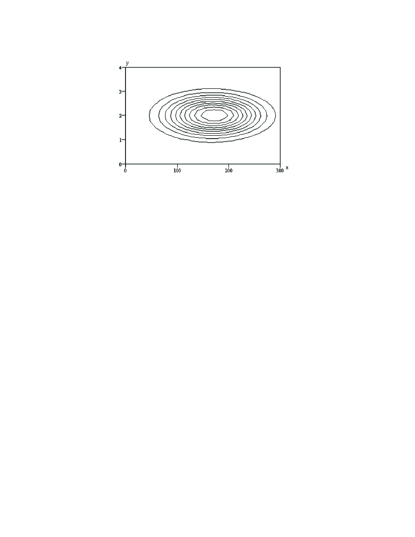
Figure 2: semiclassical Husimi function for the Morse Potential, $U(x)=D(e^{-2\alpha x}-2e^{-\alpha x}),$ where $x=\frac{r-r_{0}}{r_{o}}.$ We have used the experimental hydrogen molecule values, $\alpha=1.440$ and $D=4.75(eV).$ The principal quantum number n=0 and the angular momentum L=0. The x axis is related to the position, r, as $r=r_{0}\frac{(x+10)}{250}$, the momentum p is related to the y axis variable as $p=m\omega r_{0}\frac{(y-2)}{1.2}.$ We have used $r_{0}=7.42\times 10^{-11}m$ and $\omega=$8.3$\times$10¹⁴rad/s.

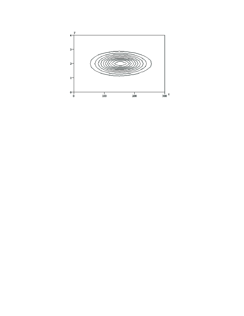
Figure 3: Husimi function for the Morse Potential with the same parameters of figure(2)

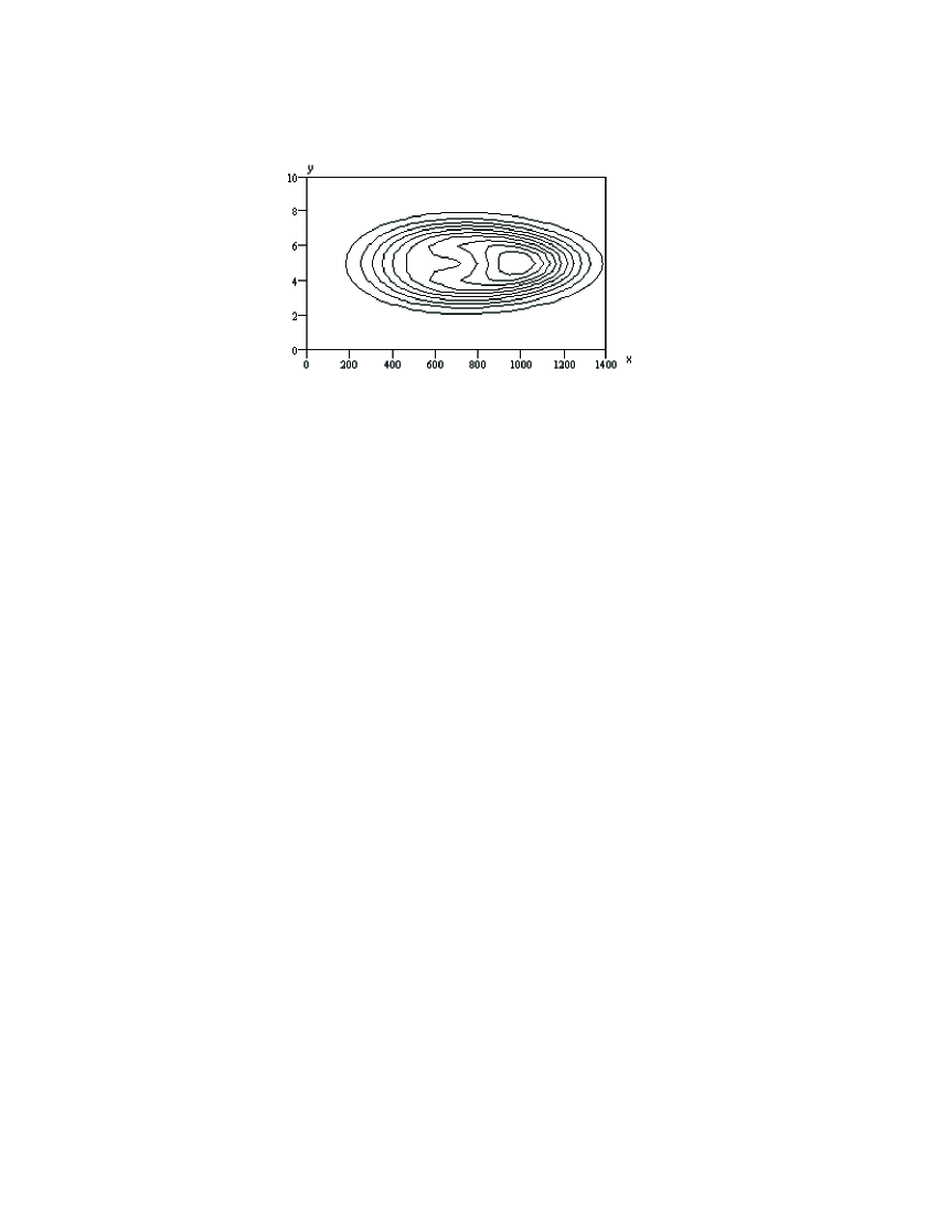
Figure 4: Semiclassical Husimi function for the Morse Potential, $U(x)=D(e^{-2\alpha x}-2e^{-\alpha x}),$ where $x=\frac{r-r_{0}}{r_{o}}.$ We have used the experimental hydrogen molecule values, $\alpha=1.440$ and $D=4.75(eV).$ The principal quantum number n=1 and the angular momentum L=0. The x axis is related to the position, r, as $r=r_{0}\frac{(x+300)}{1000}$, the momentum p is related to the y axis variable as $p=m\omega r_{0}\frac{(y-5)}{5}.$ We have used $r_{0}=7.42\times 10^{-11}m$ and $\omega=$8.3$\times$10¹⁴rad/s

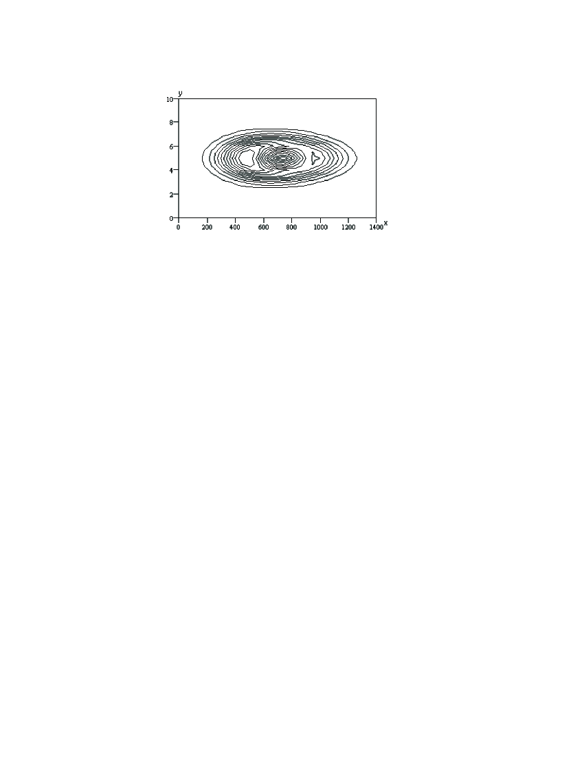
Figure 5: Husimi function for the Morse Potential with the same parameters of figure(4)

In figure (2) we show the approximated Husimi for the Morse potential with the parameters of the $H_{2}$ molecule, for $n=0$. In figure (3) we have the exact result, figure (4) shows the semiclassical Husimi function for n=1 and figure (5) the exact result, details about exact calculation can be found in ref. [8] . As we can observe in this figures, (2) and (3), the semiclassical Husimi function does not reproduce exactly the Husimi function, but it regards some similarities.

Now consider the Harmonic potential, thus we have

$$Q(t)=Q(0)cos(\omega t)+\frac{P(0)}{\omega}sin(\omega t)$$ (40)

and

$$P(t)=P(0)cos(\omega t)-Q(0)\omega sin(\omega t)$$ (41)

We chose a coordinate system such as the Hamiltonian can be written as

$$H=\omega\frac{(Q^{2}+P^{2})}{2}.$$ (42)

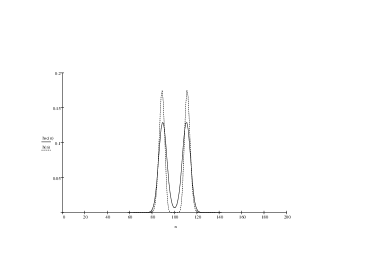
Figure 6: Full line shows a cross section of Husimi function for the harmonic potential for p=0. The principal quantum number n=5. The x axis is related to the position. Dotted line, correspondent semiclassical Husimi function.

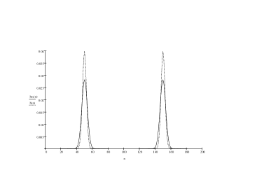
Figure 7: Full line shows a cross section of Husimi function for the harmonic potential for p=0. The principal quantum number n=100. The x axis is related to the position. Dotted line, correspondent semiclassical Husimi function.

Substituting (40) and (41) into (38) we obtain a semiclassical Husimi Function for the Harmonic oscillator with an energy $E_{n}=\hbar\omega(n+\frac{1}{2})$, without any lost of generality we can use $Q(0)=(2E_{n})^{\frac{1}{2}}$, and $P(0)=0$. In figure (6) we show the approximated and exact Husimi for the Harmonic potential for n=5. Figure (7) shows the semiclassical and exact Husimi function for n=100. In the figures (3) to (9). In order to quantify the quality of the approximation we define the function $\Delta\textbf{Q}_{\psi_{n}}(q)$ as

$$\Delta\textbf{Q}_{\psi_{n}}(q)=\textbf{H(q,p=0)}-\textbf{H(q,p=0)}_{sc},$$ (43)

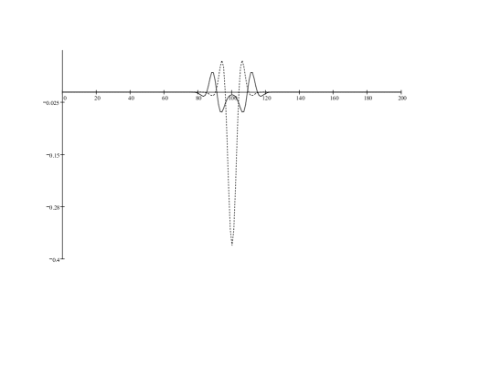
Figure 8: Dotted line shows $Q_{d}$ function for the harmonic oscillator with the principal quantum number n=1, full line n=5. X axis corresponds to position.

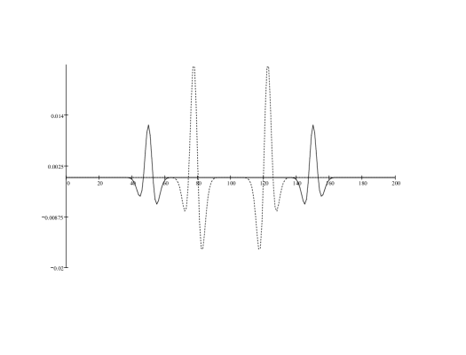
Figure 9: Dotted line shows $\Delta Q_{d}$ function for the harmonic oscillator with the principal quantum number n=20, full line n=100. X axis corresponds to position.

where H is the exact Husimi function and $\textbf{H}_{sc}$ is the semiclassical Husimi function. In Figure (8) we show $\Delta\textbf{Q}_{\psi_{n}}(q)$, for n=1 and n=5. Figure (9) same graph for n=20 and n=100. Due to the spherical symmetry we have chosen p=0. X axis corresponds to position. As we increase the principal quantum number (n) we have $\Delta\textbf{Q}_{\psi_{n}}(q)\rightarrow 0$. In order to see the classical limit, let us define the function $SQ_{\psi_{n}}$, witch is

$$SQ_{\psi_{n}}=\int_{-\infty}^{\infty}{\left|{\Delta Q}_{\psi_{n}}(q)\right|dq}$$ (44)

Suppose we have $SQ_{\psi}\approx 0$. It means that quantum description of the state $\psi$, in the Husimi’s representation, is almost contained in the semiclassical one. Of course it does not means that we have no quantum features, it only meas that Husimi is not a good observable for this situation [28]. Although that we can say that the quantum classical difference became smaller, as expected. Figure (10) shows $SQ_{n}$ for some eigenstates of the harmonic oscillator. For n=0 we have a null $SQ_{0}$, what was expected, since the fundamental harmonic oscillator eigenstate is a coherent state. Also we can say that the approximation works better as we increase the principal quantum number, as expected. From these figures we may conclude that the classical ingredient is very strong on the state formation of regular systems.

6 Semiclassical Fidelity

We now make a simple test of our approximation by applying it to a well known behavior of the fidelity. We know[20, 21, 22, 23, 24, 25] that for a linear perturbation , fidelity decays, for short times, as

$e^{-at^{2}}$ once one starts with Gaussian states. As we will see, this result is independent of the classical behavior of the system.

Let us consider  the product

$$f(\Psi,V)=\left\langle\Psi\right|U_{0}(t)U(t)\left|\Psi\right\rangle$$ (45)

where $U_{0}=e^{-\frac{i}{\hslash}Ht}$ and $U=e^{-\frac{i}{\hslash}(H+V)t},$ $V$ is a perturbation, and it is given by $V=\varepsilon\hbar(a+a^{\dagger})$ where we have $\varepsilon\ll 1$. Fidelity $(F)$ is defined as $F\equiv\left|f(\Psi,V)\right|^{2}.$  Let $\alpha(t)$ be the classical evolution of $\alpha(0)$ under the action of $H_{0\text{ }}$, and $\beta(t)$ the classical evolution of $\beta(0)$ under the action of $H=H_{0}+V.$ We consider $\beta(0)=\alpha(0).$ In this case for short times we have $\alpha(t)\approx\beta(t)+i\varepsilon t.$ Our semiclassical expansion gives

$$f(\alpha,V) = \left\langle\alpha(t)\right|\left|\beta(t)\right\rangle e^{i\left[\phi(\beta(t))-\phi(\alpha(t))\right]}$$

$$+\frac{1}{i\hbar}\int_{0}^{t}dt_{1}e^{i\eta_{3}}\left\langle\alpha(t_{1})\right|\widehat{\delta}[\alpha(t_{1})]\left|\alpha(t_{1})-i\varepsilon t\right\rangle$$

$$-\frac{1}{i\hbar}\int_{0}^{t}dt_{1}e^{i\eta_{4}}\left\langle\beta(t_{1})+\varepsilon t\right|\widehat{\delta}[\beta(t_{1})]\left|\beta(t_{1})\right\rangle+\cdot\cdot\cdot$$

The term $\left\langle\alpha(t)\right|\left|\beta(t)\right\rangle$ gives the short time behavior for $F$ and one gets

$$\left\langle\alpha(t)\right|\left|\beta(t)\right\rangle=\exp\left[-\frac{\varepsilon^{2}t^{2}}{2}-i\varepsilon t\right]$$ (46)

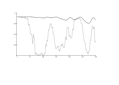
Figure 11: Semiclassical fidelity $\left|\left\langle\alpha(t)\mid\beta(t)\right\rangle\right|_{sc}^{2}$, for the driven oscillator, $\ddot{x}+x^{3}=\gamma sin(\omega t)$, with $\gamma=1$. Chaotic, $\omega=1.88$, initial condition (dotted line) $(x_{1},\dot{x}_{1})=(0,0)$. Regular, $\omega=3.88$, same initial conditions (continuous line). Both curves with the same pertubation potential. X axis corresponds to time.

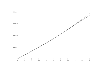
Figure 12: Semiclassical overlap $\sqrt{ln{\left|\left\langle\alpha(t)\mid\beta(t)\right\rangle\right|_{sc}^{2}}}$ , for the driven oscillator, $\ddot{x}+x^{3}=\gamma sin(\omega t)$, with $\gamma=1$. Chaotic, $\omega=1.88$, initial condition (dotted line) $(x_{1},\dot{x}_{1})=(0,0)$. Regular, $\omega=3.88$, same initial conditions (continuous line). Both curves with the same pertubation potential.

The above result is independent of the presence of chaos in the classical dynamics. In Figure (11) we show the product $\left|\left\langle\alpha(t)\mid\beta(t)\right\rangle\right|_{sc}^{2}$. As we can easely observe, the chaotic initial condition decay faster. Although that, the short time dynamics has a gaussian decay, figure (12) we show $\sqrt{ln{\left|\left\langle\alpha(t)\mid\beta(t)\right\rangle\right|_{sc}^{2}}}$ for short time evolution, witch is a straight line. As the first term in the semiclassical approximation is valid for longer times for integrable systems than for chaotic ones, we conclude that the gaussian regime should be valid for longer times as it was already found numerically in several examples of the literature[20, 23, 24, 25]. Let us now look at the general initial state situation, $f(\alpha,V)$ can be written as

$$\left\langle\Psi\right|U_{0}(t)U(t)\left|\Psi\right\rangle=\int\frac{d^{2}\alpha}{\pi}\int\frac{d^{2}\beta}{\pi}\left\langle\Psi\right|\left|\alpha\right\rangle\left\langle\alpha\right|U_{0}(t)U(t)\left|\beta\right\rangle\left\langle\beta\right|\left|\Psi\right\rangle$$ (47)

In the equation (47) we note that when $\alpha=\beta,$ we have $\left\langle\alpha\right|U_{0}(t)U(t)\left|\beta\right\rangle=f(\alpha,V)$ as defined in (46), and it has the same characteristics discussed above. However, the product $\left\langle\Psi\right|\left|\alpha\right\rangle\left\langle\beta\right|\left|\Psi\right\rangle\left\langle\alpha\right|U_{0}(t)U(t)\left|\beta\right\rangle$ is not expected to be very relevant when $\alpha$ is very different from $\beta,$ which is certainly true for short times. The whole analysis is weakened by the fact that the product $\left\langle\beta\mid\Psi\right\rangle$ may be important in chaotic and regular regions simultaneously. In this case it becomes very difficult to give a general estimate for the validity of (46).

7 Conclusions

As a general remark, we can say that, Overlap, Scar and short time Fidelity are strongly determined by the semiclassical dynamics, therefore we can say that the classical imprints are determinant. We also observe that overlap decay time has a very different dynamics from fidelity decay, although they are very similar in conception. In the particular harmonic case, we show that the first semiclassical term is able to reproduce the Husimi function with a increasing accuracy as we increase the principal quantum number n. We must remark that there is no demonstration that would suggest an existence of a limit procedure witch turns quantum corrections less important in terms of the proposed semiclassical expansion.

Acknowledgments: The author is grateful to Fapesb for partial financial support. The author also acknowledge M. C. Nemes and Enio Jelihovschi for helpful comments.

Appendix

Appendix A Semiclassical expansion and the Lyapunov Exponent

The semiclassical zeroth order is always a coherent state or a tensor product of coherent states,with the labels are described by classical dynamics. For a general state we have

$$\left\langle\psi|\phi\right\rangle=\left\langle\psi|\phi\right\rangle_{sc}+\text{corrections. }$$

Consider that initially the states are $\left|\psi(0)\right\rangle=\prod_{i}\left|\alpha_{i}(0)\right\rangle$ e $\left|\phi(0)\right\rangle=\prod_{i}\left|\beta_{i}(0)\right\rangle,$ where $\left|\alpha_{i}(0)\right\rangle$ e $\left|\beta_{i}(0)\right\rangle$ are coherent states. Then the zeroth semiclassical term is $\left\langle\psi(t)|\phi(t)\right\rangle_{sc}=\prod_{i}\left\langle\alpha_{i}(t)|\beta_{i}(t)\right\rangle$ . We know [12]that the overlap of coherent states is

$$\left|\left\langle\alpha_{i}\right|\left|\beta_{i}\right\rangle\right|^{2} = \exp(-\left|\alpha_{i}-\beta_{i}\right|^{2})\text{ \ \ \ \ \ \ \ \ \ \ \ \ \ \ \ \ \ \ \ \ \ \ \ \ for h(3);}$$ (48)

$$= \left[1-\frac{\left|\alpha_{i}-\beta_{i}\right|^{2}}{(1+\left|\beta_{i}\right|^{2})(1+\left|\alpha_{i}\right|^{2})}\right]^{2J}\text{ \ \ \ for su(2).}$$ (49)

The equation (49) coincides with (48) if we make $\alpha_{i}=\alpha_{i}/\sqrt{2J}$ and taking the limit $J\rightarrow\infty.$ In this situation we can say that

$$-\left|\alpha_{i}-\beta_{i}\right|^{2} = \ln(\left|\left\langle\alpha_{i}|\beta_{i}\right\rangle\right|^{2})$$

$$\left|\alpha_{i}-\beta_{i}\right| = \sqrt{2}(\ln\left|\left\langle\alpha_{i}|\beta_{i}\right\rangle\right|^{-1})^{1/2}.$$ (50)

We can also say that $\left|\alpha_{i}-\beta_{i}\right|^{2}=(x_{i}-y_{i})^{2}+(p_{xi}-p_{yi})$

${}^{2}\equiv\Delta q^{2}+\Delta p^{2}$.

The Lyaounov exponent is defined as

$$\lambda=\lim_{t\rightarrow\infty}\lim_{\Delta x(0)\rightarrow 0}\frac{1}{t}\ln\frac{\Delta x(t)}{\Delta x(0)}$$ (51)

onde $\Delta x(t)=\left|x_{1}(t)-x_{2}(t)\right|,$ where $x_{i}(t)$ is the clasical evolution for $x_{i}(0)$ as initial condition. In the above limit, we get

$$\left|\left\langle\alpha_{i}(t)|\beta_{i}(t)\right\rangle\right|^{2}=\exp\left[-\left(\Delta q(0)^{2}e^{2\lambda_{q}t}+\Delta p(0)^{2}e^{2\lambda_{q}t}\right)\right]$$

As we have $\sum_{i}\lambda_{i}=0,$ the biggest Lyapunov exponent($\lambda_{\max})$ is approximately

$$\lambda_{\max}=\lim_{t\rightarrow\infty}\lim_{\beta_{i}(0)\rightarrow\alpha_{i}(0)}\frac{1}{2t}\ln\left[\frac{\ln\left|\prod_{i}\left\langle\alpha_{i}(t)|\beta_{i}(t)\right\rangle\right|^{-1}}{\ln\left|\prod_{i}\left\langle\alpha_{i}(0)|\beta_{i}(0)\right\rangle\right|^{-1}}\right].$$

Observing this equation we may say that the Lyapunov exponent is related with the quantum nature of the system. As faster the quantum corrections are needed, i.e. how faster the product $\left|\left\langle\alpha_{i}(t)|\beta_{i}(t)\right\rangle\right|\rightarrow 0$ , bigger is the Lyapunov exponent. This behavior has already been pointed by many others [17, 16].

Figure 1: Squared modulus of the overlap between two neighbouring states $\left|\left\langle\alpha_{0}\right|\hat{U}_{sc}^{\dagger}\hat{U}_{sc}^{\prime}\left|\alpha_{0}^{\prime}\right\rangle\right|^{2}$, for the driven oscillator, $\ddot{x}+x^{3}=\beta sin(\omega t)$, with $\beta=1$. Chaotic initial conditions (continuous line), $\omega=1.88$, $(x_{1},\dot{x}_{1})=(0,0),(x_{2},\dot{x}_{2})=(0.002,0)$. Regular, same initial conditions (dotted line) for $\omega=3.88$. X axis corresponds to time.

Figure 10: $SQ_{d}$ function for the harmonic oscillator.X axis corresponds to the principal quantum number n.

References

- [1] A. C. Oliveira, M. C. Nemes, and K. F. Romero, Phys Rev. E 68, 036214 (2003).
- [2] A. Einstein, Deutsche Physikalische Gesellschaft Verhandlungen 19,82 (1917).
- [3] M.A.M. de Aguiar, Rev. Bras. Ens. Fis. 27,101 (2005).
- [4] E. B. Bogomolny, Pis’ma Zh. Eksp. Teor. Fiz. 44, 436 (1986), [JETP Lett. 44,561 (1986)].
- [5] E. B. Bogomolny, Physica D 31, 169 (1988).
- [6] E. J. Heller, Phys. Rev. Letters 53, 1515 (1984).
- [7] E. J. Heller, Quantum Chaos and Statistical Nuclear Physics, page 162, Springer, Berlin, 1983.
- [8] A. C. Oliveira and M. C. Nemes, Physica Scripta 64, 279 (2001).
- [9] W. D. Heiss1 and M. M ller, Phys. Rev. E 66, 016217 (2002).
- [10] M. Reis, M. O. Terra Cunha, A. C. Oliveira and M. C. Nemes, Phys Lett. A 344, 164 (2005).
- [11] M. C. Nemes, K. Furuya, G. Q. Pelegrino,A.C. Oliveira,M. Reis, L. SanzM. , Phys Lett. A 354, 60 (2006).
- [12] W. Zhang, H. Feng, and R. Gilmore, Rev. Mod. Phys. 62, 867 (1990).
- [13] X. Zeng, R. Eykholt and R. A. Pielke, Phys. Rev. Letters 66,3229 (1991).
- [14] K. M. Fonseca Romero, M. C. Nemes, J. G. Peixoto de Faria, and A. F. R. de Toledo Piza, Phys. Lett. A. 327, 129 (2004).
- [15] H.P.W. Gottlieb,J.C. Sprott Phys. Lett. A. 291, 385 (2001).
- [16] G. P. Berman and G. M. Zaslavsky, Physica A (Amsterdam) 91, 450 (1977).
- [17] G. P. Berman, A. M. Iomin, and G. M. Zaslavsky, Physica D , 113 (1981).
- [18] S. Tomsovic and E. J. Heller, Phys. Rev. Lett. 70, 1405 (1993).
- [19] M. V. Berry and N. L. Balazs, J. Phys A: Math. Gen 12, 625 (1979).
- [20] A. Peres, Phys. Rev. A 30, 1610 (1984).
- [21] F. M. Cucchiett, H. M. Pastawski, and D. A. Wisniacki, Decoherence as decay of the loschmidt echo in a lorentz gas, 2001, cond-mat/0102135 v2.
- [22] G. Benenti and G. Casati, Phys. Rev. E 65, 066205 (2002).
- [23] T. Prosen, Phys. Rev. E 65, 036208 (2002), quant-ph/0106149.
- [24] T. Prosen, T. H. Seligman, and M. Znidaric, Phys. Rev. A 67, 042112 (2003).
- [25] Y. S. Weinstein, S. Lloyd, and C. Tsallis, The edge of quantum chaos, 2002, cond-mat/0206039 v1.
- [26] Gutzwiller, M. C. “ Chaos in Classical and Quantum Mechanics, Spring-Verlg, New York (1990), Vol 1, pp. 249.
- [27] W. P Scleichr, Quantum Optics in Pahse Space, Wiley-VCC, Berlin,(2001).
- [28] A. C. Oliveira and J. G. Peixoto de Faria and M. C. Nemes, Phys Rev. E 73, 046207 (2006).
- [29] O. Bohigas, M.-J. Giannoni, and C. Schmit, Phys Rev. Letters, 52,1-4 (1984).
- [30] D. Wintgen, Phys Rev. Letters, 58,1589 (1987).
- [31] F. Haake, Quantum Signatures of Chaos, Springer-Verlag, Berlin,(2004).
- [32] F. Haake, Quantum Chaos an Introduction, Cambridge, New York,(1999).