Purifying GHZ States Using Degenerate Quantum Codes

Abstract

Degenerate quantum codes are codes that do not reveal the complete error syndrome. Their ability to conceal the complete error syndrome makes them powerful resources in certain quantum information processing tasks. In particular, the most error-tolerant way to purify depolarized Bell states using one-way communication known to date involves degenerate quantum codes. Here we study three closely related purification schemes for depolarized GHZ states shared among $m\geq 3$ players by means of degenerate quantum codes and one-way classical communications. We find that our schemes tolerate more noise than all other one-way schemes known to date, further demonstrating the effectiveness of degenerate quantum codes in quantum information processing.

I Introduction

Quantum error correcting codes, unlike their classical counterparts, may not reveal the complete error syndrome. Codes with this property are known as degenerate codes Shor and Smolin (1996); DiVincenzo et al. (1998). In a sense, degenerate codes pack more information than non-degenerate ones because different quantum errors may not take the code space to orthogonal spaces. By carefully utilizing the degenerate property, degenerate codes are useful resources in quantum information processing. Examples showing their usefulness were provided by Shor and his co-workers Shor and Smolin (1996); DiVincenzo et al. (1998). In particular, they showed that a carefully constructed degenerate code is able to purify Bell states passing through a depolarizing channel with fidelity greater than 0.80944 DiVincenzo et al. (1998). Their scheme is more error-tolerant than all the known one-way depolarized Bell state purification schemes involving non-degenerate codes to date.

It is instructive to ask if the degenerate codes can be used to improve the error-tolerant level of existing one-way multipartite purification protocols. Here we provide such an example by considering the purification of shared GHZ states. Specifically, suppose that a player prepares many copies of perfect GHZ state in the form

$$\left|\Phi^{m+}\right\rangle\equiv\frac{1}{\sqrt{2}}\left(\left|0^{\otimes m}\right\rangle+\left|1^{\otimes m}\right\rangle\right)~{}.$$ (1)

For each perfect GHZ state, he/she keeps one of the qubit and sends the other to the remaining players through a depolarizing channel so that upon reception of their qubits, these $m$ players share copies of Werner state

$$W_{F}=F\left|\Phi^{m+}\right\rangle\left\langle\Phi^{m+}\right|+\frac{1-F}{2^{m}-1}\left(I-\left|\Phi^{m+}\right\rangle\left\langle\Phi^{m+}\right|\right)~{},$$ (2)

where $F$ is the fidelity of the channel and $I$ is the identity operator. Now, the players wanted to distill shared perfect GHZ states using an one-way purification scheme that works for as small a channel fidelity as possible. Clearly, this task is a generalization of the Bell state distillation problem investigated by Shor and his co-workers Shor and Smolin (1996); DiVincenzo et al. (1998).

We begin our study by defining a few notations and reviewing prior arts in Sec. II. Then we introduce three closely related one-way multipartite purification protocols involving concatenated degenerate codes and analyze their performances in Sec. III. Actually, all three protocols use the same repetition code as their inner codes. Moreover, in the case of $m=2$, one of the our protocols is a generalization of the scheme proposed by DiVincenzo et al. DiVincenzo et al. (1998). Most importantly, for $m\geq 3$, our protocols are the most error tolerant ones discovered so far in the sense that ours can distill shared GHZ states from copies of Werner state in the form of Eq. (2) with a fidelity $F$ so low that no other one-way purification schemes known to date can. Our schemes can also be generalized to the case when the Hilbert space dimension of each quantum particle is greater than 2. We briefly discuss this issue in Sec. IV. Finally, we summarize our findings in Sec. V.

II Prior Arts

II.1 Some notations

Given that $m\geq 2$ players share $N$ noisy GHZ states in the form of Eq. (1). Clearly, the GHZ state is stabilized by its stabilizer generators, namely,

$$S_{0} = X_{0}X_{1}\cdots X_{m-1}~{},$$

$$S_{i} = Z_{0}Z_{i}$$ (3)

for $1\leq i\leq m-1$, where

$$X_{i}=\left(\begin{array}[]{cc}0&1\\ 1&0\end{array}\right)~{},Z_{i}=\left(\begin{array}[]{cc}1&0\\ 0&-1\end{array}\right)$$ (4)

denote the spin flip and phase shift operation acting on the $i$th qubit respectively. For simplicity, we use the shorthand notation $(\beta,\boldsymbol{\alpha})\equiv(\beta,\alpha_{1},\alpha_{2},\ldots,\alpha_{m-1})\in GF(2)\times GF(2)^{m-1}$ to denote the eigenvalues of stabilizer generators. Here $\beta\in GF(2)$ is the eigenvalue of the operator $S_{0}$, namely, the phase error detected; and $\alpha_{i}\in GF(2)$ is the eigenvalue of the operator $S_{i}$, namely, the bit flip error detected, for $1\leq i\leq m-1$. We sometimes abuse the notation to denote a state by $(\beta,\boldsymbol{\alpha})$. That is, we denote the states $(|0^{\otimes m}\rangle+|1^{\otimes m}\rangle)/\sqrt{2}$ and $(|0^{\otimes m}\rangle-|1^{\otimes m}\rangle)/\sqrt{2}$ by $(\beta,\boldsymbol{\alpha})=(0,\boldsymbol{0})$ and $(\beta,\boldsymbol{\alpha})=(1,\boldsymbol{0})$ respectively.

II.2 Depolarization to the GHZ-basis diagonal states

The $m$ players can depolarize each copy of their shared GHZ state into the GHZ diagonal basis using local operation and classical communication (LOCC) in the following way Dür et al. (1999). A player randomly chooses an operator from the span of the set of stabilizer generators of the GHZ state and broadcast his/her choice to the other players. Then they collectively apply the chosen operator to the GHZ state. Since all stabilizer generators of the GHZ state in Eq. (II.1) are tensor products of local unitary operators $X_{i}$ or $Z_{i}$, the players can apply the operator chosen above to the state locally using LOCC. Then, they forget which operator they have chosen. The resultant state is diagonal in the GHZ basis. Moreover, the error rate of the GHZ state is unchanged in this process. So, we can always assume that each state shared among the players are diagonal in the GHZ basis.

Among all GHZ-basis diagonal states with a fixed error rate (and hence also among all states with a fixed error rate), Werner state is the most difficult to work on as far as distillation of GHZ states is concerned. This is because one can turn any state into a Werner state with the same error rate via a depolarizing channel. Hence, to study the worst case performance of the distillation of GHZ states, we suffices to investigate the case in which the input states are Werner states.

II.3 Maneva and Smolin’s multi-party hashing protocol and its generalization by Chen and Lo

Maneva and Smolin Maneva and Smolin (2002) proposed a multi-party hashing protocol by generalizing the bilateral quantum XOR (BXOR) operation Bennett et al. (1996) to the multipartite case. In their scheme, the $m$ players carefully choose two (classical) random hashing codes, one to correct spin flip errors and the other to correct phase errors, and apply them to their shared noisy GHZ states. This can be done by using local operation plus classical communication with the help of a few multi-lateral quantum XOR (MXOR) operations. Recall that MXOR is a linear map transforming the state $\bigotimes_{i=0}^{m-1}|j_{i},k_{i}\rangle_{i}$ to $\bigotimes_{i=0}^{m-1}|j_{i},j_{i}+k_{i}\rangle_{i}$ for all $j_{i},k_{i}\in GF(2)$. Here, quantum particles with subscript $i$ belong to the $i$th player. Suppose the source and target states are eigenstates of the stabilizer generator in Eq. (II.1) with eigenvalues $(\beta_{1},\boldsymbol{\alpha}_{1})$ and $(\beta_{2},\boldsymbol{\alpha}_{2})$ respectively. Then after the MXOR operation, the resultant state is also an eigenstate of the stabilizer generator with eigenvalues Maneva and Smolin (2002)

$$\text{MXOR}[(\beta_{1},\boldsymbol{\alpha}_{1}),(\beta_{2},\boldsymbol{\alpha}_{2})]=[(\beta_{1}+\beta_{2},\boldsymbol{\alpha}_{1}),(\beta_{2},\boldsymbol{\alpha}_{1}-\boldsymbol{\alpha}_{2})]~{}.$$ (5)

Using the observation that spin flip error occurred in different qubit of a GHZ state can be detected and corrected in parallel, Maneva and Smolin showed that the asymptotic yield of their hashing protocol in the limit of large number of shared noisy GHZ states is given by Maneva and Smolin (2002)

$$D_{1}=1-\max_{1\leq i\leq m-1}[{H(b_{i})}]-H(b_{0})~{},$$ (6)

where $H(x)\equiv-\sum_{j}p_{j}\log_{2}p_{j}$ is the classical Shannon entropy function. Here the $n$-bit string $b_{0}$ represents the random choice of $\beta_{1},\ldots,\beta_{N}$ where $\beta_{\ell}$ corresponds to the eigenvalue of the operator $S_{0}$ of the $\ell$th GHZ-state $\left|\Phi^{m+}\right\rangle$’s and the $N$-bit string $b_{i}$ represents the random choice of $\alpha_{1i},\ldots,\alpha_{Ni}$ where $\alpha_{\ell i}$ is the eigenvalue of the operator $S_{i}$ of the $\ell$th GHZ state for $1\leq i\leq m-1$. That is to say, $H(b_{0})$ is the averaged phase error rate and $H(b_{i})$ is the averaged bit flip rate corresponding to the stabilizer generator $S_{i}$ (for $i=1,2,\ldots,m-1$) over the $N$ GHZ states respectively.

Recently, Chen and Lo improved the above random hashing protocol by exploiting the correlation between the string $b_{i}$. Specifically, they replaced the spin flip error-correction random hashing code used in Maneva and Smolin protocol by the following scheme. (Actually, they only considered the case of three players. What we report below is a straight-forward generalization to the case of $m$ players as we need to use this generalization later on.) Player 1 applies (classical) random hashing to correct spin flip error occurred in his/her share of the GHZ states. He/She then broadcasts his/her hashing code used and his measurement results. For $i=2,\ldots,m-1$, the $i$th player carefully picks his/her (classical) random hashing code to correct spin flip error occurred in his/her share of the GHZ states based on the broadcast information of players $1,2,\ldots,i-1$. Then, the $i$th player broadcasts his/her code used and his/her measurement results. In this way, the yield of Maneva and Smolin scheme can be increased to Chen and Lo (2007)

$$D_{2} = 1-\max\{H(b_{1}),H(b_{2}|b_{1}),H(b_{3}|b_{2},b_{1}),\cdots,H(b_{m-1}|b_{m-2},b_{m-3},\ldots,b_{1})\}$$ (7)

$$~{}-H(b_{0})+I(b_{0};b_{m-1},b_{m-2},\ldots,b_{1})$$

where the function $I(\,;\,)$ is the mutual information between the two classical random variables appear in its arguments.

Applying the random hashing method of Maneva and Smolin to a collection of identical tripartite (that is, $m=3$) Werner states in Eq. (2), one can obtain perfect GHZ state with non-zero yield whenever the fidelity $F\geq 0.8075$ Maneva and Smolin (2002). Using the Chen and Lo’s formula in Eq. (7), one can push this threshold fidelity down to $0.7554$ Chen and Lo (2007).

II.4 Shor-Smolin concatenation procedure and its generalization to the multipartite situation

Built on an earlier work by Shor and Smolin Shor and Smolin (1996), DiVincenzo et al. introduced a highly error-tolerant way of distilling shared Bell states by means of a concatenation procedure DiVincenzo et al. (1998). This procedure can be generalized to distill shared GHZ states in a straight-forward manner. We report this generalization below since we have to use a few related equations later on.

Suppose $m$ players share $Nn$ copies of imperfect GHZ states for $N\gg 1$. They perform the following two level decoding procedure. First, the players randomly divide these GHZ states into $N$ equal parts. Then each player applies a decoding transformation associated with an additive $[n,k_{1},d_{1}]$ code to his/her own qubits followed by the error syndrome measurements. Surely, this can be done with the help of a few MXOR operations. By comparing the difference in player’s measurement results, they obtain the syndrome $\vec{\boldsymbol{s}}\in GF(2)^{(m-1)(n-k_{1})}$. To continue, each party applies another decoding transformation corresponding to a (classical) random hashing code $[Nk_{1},k_{2},d_{2}]$ to correct errors in the GHZ diagonal basis and broadcast the measurement results. Finally, they apply the necessary unitary transformation according to the measured error syndrome of this random hashing code to get the purified GHZ states.

Suppose that an additive code $[n,k_{1},d_{1}]$ is applied and the remaining states after the decoding transformation and measurements are denoted by $(\delta,\boldsymbol{\gamma})\equiv\text{TRAN}[(\beta_{1},\boldsymbol{\alpha}_{1}),(\beta_{2},\boldsymbol{\alpha}_{2}),\ldots,(\beta_{k_{1}},\boldsymbol{\alpha}_{k_{1}})]$. Then, the yield of this concatenated scheme is given by the so-called Shor-Smolin capacity Shor and Smolin (1996); DiVincenzo et al. (1998)

$$D_{\textrm{SS}}=\frac{1}{n}(1-S_{X})~{},$$ (8)

where

$$S_{X}=\sum_{\vec{\boldsymbol{s}}\in GF(2)^{(m-1)(n-k_{1})}}\text{Pr}(\vec{\boldsymbol{s}})\enspace h(\{\text{Pr}((\delta,\boldsymbol{\gamma})|\vec{\boldsymbol{s}}):(\delta,\boldsymbol{\gamma})\in GF(2)^{m}\})$$ (9)

is the average of the von Neumann entropies of the quantum states conditional on the measurement outcomes. Note that in Eq. (9), $\text{Pr}(\vec{\boldsymbol{s}})$ is the probability that the measurement outcome is $\vec{\boldsymbol{s}}$,

$$h(\{p_{i}\})\equiv-\sum_{i}p_{i}\log_{2}p_{i}~{},$$ (10)

and

$$\sum_{i}p_{i}=1~{}.$$ (11)

By applying the above procedure to depolarized Bell states using a 5-qubit cat code as the inner code and a random hashing code as the outer code (that is, the case of $m=2$ and $n=5$), DiVincenzo et al. found that one can attain a non-zero capacity whenever the channel fidelity $F>0.80944$ DiVincenzo et al. (1998). Since the performance of this scheme exceeds that of quantum random hashing code and that the 5-qubit cat code is degenerate, the power of using degenerate quantum code in quantum information processing is demonstrated.

II.5 Other hashing and breeding schemes

Several other multipartite hashing schemes have been studied Maneva and Smolin (2002); Hostens et al. (2006a). In particular, Maneva and Smolin’s hashing scheme can distill shared GHZ states from copies of Werner states with fidelity $F\geq 0.7798$ in the limit of arbitrarily large number of players (that is, when $m\rightarrow\infty$) Maneva and Smolin (2002). Another approach is to use the so-called stabilizer breeding. In particular, Hostens et al. showed that stabilizer breeding is able to purify depolarized $5$-qubit ring state with fidelity $F\geq 0.756$ Hostens et al. (2006b). A few authors also studied the distillation of graph state subjected to local $Z$-noise Kay et al. (2006) and bicolorable graph state. Goyal et al. (2006) Furthermore, Glancy et al. generalized the hashing protocol of Maneva and Smolin to purify a much larger class of output state. Glancy et al. (2006) The second column in Table 1 summarizes the state-of-the-art one-way purification schemes to distill depolarized GHZ states before our work.

$m$	prior art	our best protocol	lower bound
2	0.8094	0.8094	0.7500
3	0.7554	0.7074	0.6111
4	0.7917	0.6601	0.5500

Table 1: The threshold fidelity of the depolarizing channel above which a GHZ state can be distilled by prior art and by our protocols. Also listed is the lower bound of the fidelity below which no one-way protocol can distill shared GHZ state using Eq. (43) in Sec. III.5. As for prior art, the threshold fidelity for $m=2$ is given by the 5-qubit cat code DiVincenzo et al. (1998). For $m=3$ case, the threshold is computed by the Chen and Lo’s formula Chen and Lo (2007) in Eq. (7). For $m=4$, the threshold is given by the Maneva and Smolin’s hashing protocol Maneva and Smolin (2002) in Eq. (6).

III Our protocols involving degenerate code and their performances

III.1 Our protocols

Our three protocols are natural extensions of the Shor-Smolin concatenation procedure to the case of purifying GHZ states. They all use the same degenerate quantum code as the inner code. Specifically, suppose the $m$ players share $Nn$ copies of Werner state with $N\gg 1$. As shown in Fig. 1, to distill perfect GHZ state, each player applies the (classical) $[n,1,n]$ repetition code, whose stabilizer generators are

$$Z_{0}Z_{1},Z_{0}Z_{2},\ldots,Z_{0}Z_{n-1}~{},$$ (12)

to his/her own $n$ qubits. That is to say, they randomly partition the $Nn$ shared noisy GHZ states into $N$ sets, each containing $n$ noisy GHZ states. In each set ${\mathfrak{S}}$, they randomly assign one of the noisy GHZ state as the source (and call it the $0$th copy of $\left|\Phi^{m+}\right\rangle$ in the set) and the remaining $(n-1)$ noisy GHZ states as the targets (and call them the $j$th copy of $\left|\Phi^{m+}\right\rangle$ in the set for $j=1,2,\ldots,n-1$). They apply the MXOR operation to copies of $\left|\Phi^{m+}\right\rangle$ in each set and then measure all the target GHZ states in the standard computational basis while leaving all the source GHZ states un-measured. We denote the syndrome and the remaining state in each set by $\vec{\boldsymbol{s}}_{\mathfrak{S}}\in GF(2)^{(n-1)(m-1)}$ and $(\delta_{\mathfrak{S}},\boldsymbol{\gamma}_{\mathfrak{S}})\in GF(2)^{m}$ respectively. (Since the partition into $N$ sets is arbitrarily chosen and our subsequent analysis only makes use of the statistical properties of the states in each set, we drop the set label ${\mathfrak{S}}$ in all quantities to be analyzed from now on.)

Our three protocols differ in the use of outer codes. For the first protocol, each player applies a (classical) random hashing code $[N,k_{2},d_{2}]$ that corrects GHZ diagonal basis errors to the $N$ remaining states (each coming from a different set ${\mathfrak{S}}$) and exchanges the measurement results. Clearly, this protocol is reduced to the Shor-Smolin concatenation procedure Shor and Smolin (1996) when $m=2$.

Figure 1: Our three GHZ state distillation protocols for $m=n=3$. They all use the $[n,1,n]$ repetition code as their inner codes; and they differ by the kind of random hashing outer code used.

For the second protocol, the players follow Maneva and Smolin’s idea Maneva and Smolin (2002) by using two (classical) random hashing codes, one to correct spin flip error and the other to correct phase shift. In this sense, the outer code used in our second protocol is a random asymmetric Calderbank-Shor-Steane (CSS) code. Whereas players in our third protocol use the Chen and Lo’s generalization Chen and Lo (2007) as their outer code. That is, the outer code is a random asymmetric CSS code whose decoding circuit is carefully designed to exploit the correlation between the bit string $b_{i}$.

In all the above three protocols, the players have to apply the corresponding unitary transformation for the outer code to obtain the purified GHZ states. (See Fig. 1.)

Clearly, the yield of the first protocol is the Shor-Smolin capacity given by Eqs. (8) and (9). And by applying Eq. (6) to the noisy GHZ state to be fed into the outer code of the second protocol, we conclude that the yield of the second protocol equals

$$D_{\textrm{MS}}=\frac{1}{n}\left(1-\sum_{\vec{\boldsymbol{s}}\in GF(2)^{(m-1)(n-1)}}\textrm{Pr}(\vec{\boldsymbol{s}})\left\{\max_{1\leq i\leq m-1}\left[H(\gamma_{i}|\vec{\boldsymbol{s}})\right]+H(\delta|\vec{\boldsymbol{s}})\right\}\right)$$ (13)

where

$$H(\gamma_{i}|\vec{\boldsymbol{s}})=h(\{\sum_{\delta,\gamma_{1},\ldots,\gamma_{i-1},\gamma_{i+1},\ldots,\gamma_{m-1}\in GF(2)}\textrm{Pr}((\delta,\boldsymbol{\gamma})|\vec{\boldsymbol{s}}):\gamma_{i}\in GF(2)\})$$ (14)

for $i=1,2,\ldots,m-1$, and

$$H(\delta|\vec{\boldsymbol{s}})=h(\{\sum_{\boldsymbol{\gamma}\in GF(2)^{m-1}}\textrm{Pr}((\delta,\boldsymbol{\gamma})|\vec{\boldsymbol{s}}):\delta\in GF(2)\}).$$ (15)

Similarly, from Eq. (7), the yield of the third protocol is

$$D_{\textrm{CL}}=\frac{1}{n}\left(1-\sum_{\vec{\boldsymbol{s}}\in GF(2)^{(m-1)(n-1)}}\textrm{Pr}(\vec{\boldsymbol{s}})\left\{\max_{1\leq i\leq m-1}\left[H(\gamma_{i}|\gamma_{i-1},\gamma_{i-2},\ldots,\gamma_{1},\vec{\boldsymbol{s}})\right]+H(\delta|\vec{\boldsymbol{s}})-I(\delta;\boldsymbol{\gamma}|\vec{\boldsymbol{s}})\right\}\right)$$ (16)

where

$$H(\gamma_{i}|\gamma_{i-1},\gamma_{i-1},\ldots,\gamma_{1},\vec{\boldsymbol{s}})=h(\{\sum_{\delta,\gamma_{i+1},\gamma_{i+2},\ldots,\gamma_{m-1}\in GF(2)}\textrm{Pr}((\delta,\boldsymbol{\gamma})|\gamma_{i-1},\gamma_{i-2},\ldots,\gamma_{1},\vec{\boldsymbol{s}}):\gamma_{i}\in GF(2)\})$$ (17)

for $i=1,2,\ldots,m-1$ and $I(\delta;\boldsymbol{\gamma}|\vec{\boldsymbol{s}})$ is the conditional mutual information between $\delta$, and $\boldsymbol{\gamma}$ given $\vec{\boldsymbol{s}}$.

III.2 Evaluating the yields for Werner states for our protocols

To analyze the performance of our three protocols when applied to Werner states, we first have to calculate the distribution of outcomes after passing the Werner states through the inner repetition code. For an arbitrary but fixed set ${\mathfrak{S}}$, using the compact notation introduced in Sec.II, we denote the error experienced by the $j$th copy of $\left|\Phi^{m+}\right\rangle$ in this set by $(\beta_{j},\boldsymbol{\alpha}_{j})$ for $j=0,1,\ldots,n-1$. After decoding the inner code, namely, the $[n,1,n]$ repetition code whose generators of the stabilizer are written down in Eq. (12), the syndrome $\vec{\boldsymbol{s}}\equiv(\boldsymbol{s}_{1},\boldsymbol{s}_{2},\ldots\boldsymbol{s}_{n-1})\in GF(2)^{(m-1)(n-1)}$ obtained obeys

$$\boldsymbol{s}_{j}\equiv\boldsymbol{\alpha}_{j}-\boldsymbol{\alpha}_{0}\in GF(2)^{m-1}$$ (18)

for all $1\leq j\leq n-1$. Furthermore, the remaining state shared among the $m$ players is

$$(\delta,\boldsymbol{\gamma})=(\sum_{j=0}^{n-1}\beta_{j},\boldsymbol{\alpha}_{0})~{}.$$ (19)

To simplify notation in our subsequent discussions, we define

$$\boldsymbol{s}_{0}=\boldsymbol{0}$$ (20)

so that Eq. (18) is also valid for $j=0$.

To evaluate the capacity for each of our three protocols, we first have to calculate the conditional probabilities $\text{Pr}((\delta,\boldsymbol{\gamma})|\vec{\boldsymbol{s}})$ and $\textrm{Pr}((\delta,\boldsymbol{\gamma})|\gamma_{1},\gamma_{2},\ldots,\gamma_{i-1},\vec{\boldsymbol{s}})$ in Eqs. (9) and (16), respectively. We begin by computing the probability $\text{Pr}((\delta,\boldsymbol{\gamma})\wedge\vec{\boldsymbol{s}})$ that the source state has experienced the error $(\delta,\boldsymbol{\gamma})=(\sum_{j=0}^{n-1}\beta_{j},\boldsymbol{\alpha}_{0})$ after the decoding transformation of the repetition code in Eq. (12) and that the error syndrome for the repetition code is $\vec{\boldsymbol{s}}\in GF(2)^{(m-1)(n-1)}$. Clearly,

$$\text{Pr}((\delta,\boldsymbol{\gamma})\wedge\vec{\boldsymbol{s}})=\text{Pr}({\mathfrak{E}}(\vec{\boldsymbol{s}},\delta,\boldsymbol{\gamma}))$$ (21)

where

$${\mathfrak{E}}(\vec{\boldsymbol{s}},\delta,\boldsymbol{\gamma})\equiv\{(\beta_{j},\boldsymbol{\alpha}_{j})_{j=0}^{n-1}\in GF(2)^{mn}:\delta=\sum_{j=0}^{n-1}\beta_{j},\boldsymbol{\gamma}=\boldsymbol{\alpha}_{0},\boldsymbol{\alpha}_{\ell}=\boldsymbol{s}_{\ell}+\boldsymbol{\alpha}_{0}\enspace\text{for}\enspace\ell=1,2,\ldots,n-1\}~{}.$$ (22)

Since the repetition code and our decoding transformation are highly symmetric in the sense that they are invariant under relabeling of qubits, it is not surprising that the set ${\mathfrak{E}}(\vec{\boldsymbol{s}},\delta,\boldsymbol{\gamma})$ is invariant under permutation of phase errors. That is to say, $(\beta_{j},\boldsymbol{\alpha}_{j})_{j=0}^{n-1}\in{\mathfrak{E}}(\vec{\boldsymbol{s}},\delta,\boldsymbol{\gamma})$ if and only if $(\beta_{\pi(j)},\boldsymbol{\alpha}_{j})_{j=0}^{n-1}\in{\mathfrak{E}}(\vec{\boldsymbol{s}},\delta,\boldsymbol{\gamma})$ where $\pi$ is a permutation of $\{0,1,\ldots,n-1\}$.

III.2.1 Finding $\text{Pr}((\delta,\boldsymbol{\gamma})\wedge\vec{\boldsymbol{s}})$

We proceed by introducing the concepts of depolarization weight and depolarization weight enumerator similar to the ones proposed by DiVincenzo et al. DiVincenzo et al. (1998). Let $(\beta_{j},\boldsymbol{\alpha}_{j})$ be the state of the $j$th noisy GHZ state shared among the $m$ players. The depolarization weight of the order $n$-tuple $(\beta_{j},\boldsymbol{\alpha}_{j})_{j=0}^{n-1}\in GF(2)^{mn}$ is defined as its Hamming weight by regarding this $n$-tuple as a vector of elements in $GF(2)^{m}$. In other words,

$$\text{wt}\left((\beta_{j},\boldsymbol{\alpha}_{j})_{j=0}^{n-1}\right)=|\{j\in\{0,1,\ldots,n-1\}:(\beta_{j},\boldsymbol{\alpha}_{j})\neq(0,\boldsymbol{0})\}|~{}.$$ (23)

Physically, the depolarization weight measures the number of shared GHZ states that experienced an error; thus, it is invariant under permutation of the $n$ possibly imperfect GHZ states. Since a GHZ state has equal probability of having each type of error after passing through a depolarizing channel, there is an equal probability for the $n$ depolarized GHZ states to experience errors with the same depolarization weight. Thus, we may find the probability $\text{Pr}((\delta,\boldsymbol{\gamma})\wedge\vec{\boldsymbol{s}})$ by studying the depolarization weight enumerator $w({\mathfrak{E}}(\vec{\boldsymbol{s}},\delta,\boldsymbol{\gamma});x,y)$ where

$$w({\mathfrak{A}};x,y)=\sum_{\vec{\boldsymbol{a}}\in{\mathfrak{A}}}x^{\text{wt}(\vec{\boldsymbol{a}})}y^{n-\text{wt}(\vec{\boldsymbol{a}})}~{}.$$ (24)

The depolarization weight enumerator of a set is a natural generalization of the concept of weight enumerator of a code.

Finding an explicit expression for the above depolarization weight enumerator for an arbitrary set or coset is a very difficult task. It is the high degree of symmetry in the repetition code that makes this task possible. In fact, one may transform a state in ${\mathfrak{E}}(\vec{\boldsymbol{s}},\delta,\boldsymbol{\gamma})$ to another state in the same set by applying phase shifts to a few qubits.

By counting the number of different possible combinations of $(\beta_{j},\boldsymbol{\alpha}_{j})$’s subjected to the constraint that $(\beta_{j},\boldsymbol{\alpha}_{j})_{j=0}^{n-1}\in{\mathfrak{E}}(\vec{\boldsymbol{s}},\delta,\boldsymbol{\gamma})$, we have

$$w({\mathfrak{E}}(\vec{\boldsymbol{s}},\delta,\boldsymbol{\gamma});x,y)=\mathop{{\sum}^{\prime}}\frac{n!}{\displaystyle\prod_{\genfrac{}{}{0.0pt}{}{i\in GF(2),}{\boldsymbol{t}\in GF(2)^{m-1}}}a_{i,\boldsymbol{t}}!}\enspace x^{n-a_{0,\boldsymbol{0}}}y^{a_{0,\boldsymbol{0}}}$$ (25)

where the primed sum is over all $a_{i,\boldsymbol{t}}$’s satisfying the constraints

$$a_{i,\boldsymbol{t}}\geq 0\enspace\forall i,\boldsymbol{t}~{},$$ (26)

$$\sum_{\genfrac{}{}{0.0pt}{}{i\in GF(2),}{\boldsymbol{t}\in GF(2)^{m-1}}}a_{i,\boldsymbol{t}}=n~{},$$ (27)

$$\sum_{i\in GF(2)}a_{i,\boldsymbol{t}}=|\{j\in\{0,1,\ldots,n-1\}:\boldsymbol{s}_{j}+\boldsymbol{\gamma}=\boldsymbol{t}\}|\enspace\forall\boldsymbol{t}$$ (28)

and

$$\sum_{\genfrac{}{}{0.0pt}{}{i\in GF(2),}{\boldsymbol{t}\in GF(2)^{m-1}}}i\,a_{i,\boldsymbol{t}}=\delta~{}.$$ (29)

Note that the symbol $a_{i,\boldsymbol{t}}$ in the above equations can be interpreted as the number of GHZ states that experienced the error $(i,\boldsymbol{t})$ before the commencement of our distillation protocol.

Let

$$k\equiv k(\vec{\boldsymbol{s}},\boldsymbol{\gamma})=|\{j\in\{0,1,\ldots,n-1\}:\boldsymbol{s}_{j}+\boldsymbol{\gamma}\neq\boldsymbol{0}\}|$$ (30)

be the number of qubits having spin flip for each element in ${\mathfrak{E}}(\vec{\boldsymbol{s}},\delta,\boldsymbol{\gamma})$. We have two cases to consider.

Case (a) $k>0$: That is, there exists $\ell$ such that $\boldsymbol{s}_{\ell}+\boldsymbol{\gamma}\neq\boldsymbol{0}$. Hence, $\text{wt}((\beta_{j},\boldsymbol{s}_{j}+\boldsymbol{\gamma})_{j=0}^{n-1})$ is independent of the value of $\beta_{\ell}\in GF(2)$. In addition, by regarding the equation $\sum_{j=0}^{n-1}\beta_{j}=\delta$ as a bijection relating $\beta_{\ell}\in GF(2)$ and $\delta\in GF(2)$, we conclude that the depolarization weight enumerator $w({\mathfrak{E}}(\vec{\boldsymbol{s}},\delta,\boldsymbol{\gamma});x,y)$ is independent of the value of $\delta\in GF(2)$. Hence,

$$w({\mathfrak{E}}(\vec{\boldsymbol{s}},\delta,\boldsymbol{\gamma});x,y)=\frac{1}{2}\mathop{{\sum}^{\prime\prime}}\frac{n!}{\displaystyle\prod_{\genfrac{}{}{0.0pt}{}{i\in GF(2),}{\boldsymbol{t}\in GF(2)^{m-1}}}a_{i,\boldsymbol{t}}!}\enspace x^{n-a_{0,\boldsymbol{0}}}y^{a_{0,\boldsymbol{0}}}$$ (31)

where the double primed sum is over all $a_{i,\boldsymbol{t}}$’s satisfying constraints Eq. (26)–(28) only. Consequently,

$$w({\mathfrak{E}}(\vec{\boldsymbol{s}},\delta,\boldsymbol{\gamma});x,y) = \frac{1}{2}\sum_{\{a_{i,\boldsymbol{t}}\}}\frac{k!}{\displaystyle\prod_{\genfrac{}{}{0.0pt}{}{i\in GF(2),}{\boldsymbol{t}\in{GF(2)^{m-1}}\setminus\{\boldsymbol{0}\}}}a_{i,\boldsymbol{t}}}\enspace{n-k\choose a_{0,\boldsymbol{0}}}\enspace x^{n-a_{0,\boldsymbol{0}}}y^{a_{0,\boldsymbol{0}}}$$ (32)

$$= 2^{k-1}\sum_{a_{0,\boldsymbol{0}}}{n-k\choose a_{0,\boldsymbol{0}}}\enspace x^{n-a_{0,\boldsymbol{0}}}y^{a_{0,\boldsymbol{0}}}$$

$$= 2^{k-1}x^{k}(x+y)^{n-k}~{}.$$

Case (b) $k=0$: That is, $\boldsymbol{s}_{j}+\boldsymbol{\gamma}=\boldsymbol{0}$ for all $j$ so that phase shift is the only type of error a GHZ state may experience. In this case, the union of disjoint sets $\bigcup_{\delta\in GF(2)}{\mathfrak{E}}(\vec{\boldsymbol{s}},\delta,\boldsymbol{\gamma})$ is equal to the set of all possible phase errors experienced by the $n$ shared GHZ states. As a result,

$$\sum_{\delta\in GF(2)}w({\mathfrak{E}}(\vec{\boldsymbol{s}},\delta,\boldsymbol{\gamma});x,y)=w(\bigcup_{\delta\in GF(2)}{\mathfrak{E}}(\vec{\boldsymbol{s}},\delta,\boldsymbol{\gamma});x,y)=\sum_{i}{n\choose i}\enspace x^{i}y^{n-i}=(x+y)^{n}~{}.$$ (33)

Similarly,

$$\sum_{\delta\in GF(2)}(-1)^{\delta}w({\mathfrak{E}}(\vec{\boldsymbol{s}},\delta,\boldsymbol{\gamma});x,y)=w(\bigcup_{\delta\in GF(2)}{\mathfrak{E}}(\vec{\boldsymbol{s}},\delta,\boldsymbol{\gamma});-x,y)=\sum_{i}{n\choose i}\enspace(-x)^{i}y^{n-i}=(y-x)^{n}~{}.$$ (34)

(Note that the validity of the above equation follows from the observation that $\delta=1$ if and only if the number of qubits having phase shift error before the commencement of our protocol is odd. Moreover, the coefficient of $w(\{\vec{\boldsymbol{a}}\};-x,y)$ is negative if and only if $wt(\vec{\boldsymbol{a}})$ is odd.) From Eqs. (32)–(34), we conclude that

$$w({\mathfrak{E}}(\vec{\boldsymbol{s}},\delta,\boldsymbol{\gamma});x,y)\equiv w(k,\delta;x,y)=\left\{\begin{array}[]{ll}\displaystyle 2^{k-1}x^{k}(x+y)^{n-k}&\enspace\text{if}\enspace 0<k\leq n,\\ \\ \displaystyle\frac{1}{2}\left[(x+y)^{n}+(y-x)^{n}\right]&\enspace\text{if}\enspace k=0\enspace\text{and}\enspace\delta=0,\\ \\ \displaystyle\frac{1}{2}\left[(x+y)^{n}-(y-x)^{n}\right]&\enspace\text{if}\enspace k=0\enspace\text{and}\enspace\delta\neq 0,\end{array}\right.$$ (35)

where $k=k(\vec{\boldsymbol{s}},\boldsymbol{\gamma})$ is the number of GHZ states that experienced some kind of spin flip for each of the state in ${\mathfrak{E}}(\vec{\boldsymbol{s}},\delta,\boldsymbol{\gamma})$ as defined by Eq. (30).

Recall that ${\mathfrak{E}}(\vec{\boldsymbol{s}},\delta,\boldsymbol{\gamma})$ is invariant under permutation of phase errors among the $n$ GHZ states. Moreover, both the depolarization weight and the value of $k(\vec{\boldsymbol{s}},\boldsymbol{\gamma})$ are invariant under permutation of the $n$ GHZ states. So, it is not surprising that the depolarizing weight enumerator $w({\mathfrak{E}}(\vec{\boldsymbol{s}},\delta,\boldsymbol{\gamma});x,y)$ depends only on the values of $k$ and $\delta$. Therefore, our shorthand notation $w(k,\delta;x)$ makes sense.

From Eq. (21) and by substituting $x=(1-F)/(2^{m}-1)$, $y=F$ into Eq. (35), we find that

$$\text{Pr}((\delta,\boldsymbol{\gamma})\wedge\vec{\boldsymbol{s}})=\left\{\begin{array}[]{ll}\displaystyle\frac{2^{k-1}(1-F)^{k}(2^{m}F-2F+1)^{n-k}}{(2^{m}-1)^{n}}&\enspace\text{if}\enspace 0<k\leq n,\\ \\ \displaystyle\frac{(2^{m}F-2F+1)^{n}+(2^{m}F-1)^{n}}{2(2^{m}-1)^{n}}&\enspace\text{if}\enspace k=0\enspace\text{and}\enspace\delta=0,\\ \\ \displaystyle\frac{(2^{m}F-2F+1)^{n}-(2^{m}F-1)^{n}}{2(2^{m}-1)^{n}}&\enspace\text{if}\enspace k=0\enspace\text{and}\enspace\delta\neq 0.\end{array}\right.$$ (36)

for a depolarizing channel with fidelity $F$. Note that by fixing the number of players $m$, the number of noisy GHZ states shared between the players $n$ and the fidelity of the depolarizing channel $F$, the probability $\text{Pr}((\delta,\boldsymbol{\gamma})\wedge\vec{\boldsymbol{s}})$ can take on at most $(n+2)$ different values.

III.2.2 Finding $\text{Pr}((\delta,\boldsymbol{\gamma})|\vec{\boldsymbol{s}})$

Clearly

$$\text{Pr}(\vec{\boldsymbol{s}})=\sum_{\boldsymbol{t}\in GF(2)^{m-1}}\text{Pr}(\vec{\boldsymbol{s}}\wedge\boldsymbol{t})$$ (37)

where $\text{Pr}(\vec{\boldsymbol{s}}\wedge\boldsymbol{t})$ is the probability that the error experienced by the $n$ noisy GHZ states is $(\beta_{j},\boldsymbol{s}_{j}+\boldsymbol{t})_{j=0}^{n-1}$ for $\beta_{j}\in GF(2)$. For a depolarizing channel with fidelity $F$,

$$\text{Pr}(\vec{\boldsymbol{s}}) = \sum_{\boldsymbol{t}\in GF(2)^{m-1}}\left[\frac{2(1-F)}{2^{m}-1}\right]^{k(\vec{\boldsymbol{s}},\boldsymbol{t})}\enspace\left(F+\frac{1-F}{2^{m}-1}\right)^{n-k(\vec{\boldsymbol{s}},\boldsymbol{t})}$$ (38)

$$= \frac{1}{(2^{m}-1)^{n}}\sum_{i=0}^{n}f_{\vec{\boldsymbol{s}}}(i)2^{i}(1-F)^{i}(2^{m}F-2F+1)^{n-i}$$

where

$$f_{\vec{\boldsymbol{s}}}(i)=|\{\boldsymbol{t}\in GF(2)^{m-1}:k(\vec{\boldsymbol{s}},\boldsymbol{t})=i\}|~{}.$$ (39)

Therefore,

$$\text{Pr}((\delta,\boldsymbol{\gamma})|\vec{\boldsymbol{s}})=\left\{\begin{array}[]{ll}\displaystyle\frac{2^{k-1}(1-F)^{k}(2^{m}F-2F+1)^{n-k}}{\sum_{i}f_{\vec{\boldsymbol{s}}}(i)2^{i}(1-F)^{i}(2^{m}F-2F+1)^{n-i}}&\enspace\text{if}\enspace 0<k\leq n,\\ \\ \displaystyle\frac{(2^{m}F-2F+1)^{n}+(2^{m}F-1)^{n}}{2\sum_{i}f_{\vec{\boldsymbol{s}}}(i)2^{i}(1-F)^{i}(2^{m}F-2F+1)^{n-i}}&\enspace\text{if}\enspace k=0\enspace\text{and}\enspace\delta=0,\\ \\ \displaystyle\frac{(2^{m}F-2F+1)^{n}-(2^{m}F-1)^{n}}{2\sum_{i}f_{\vec{\boldsymbol{s}}}(i)2^{i}(1-F)^{i}(2^{m}F-2F+1)^{n-i}}&\enspace\text{if}\enspace k=0\enspace\text{and}\enspace\delta\neq 0.\end{array}\right.$$ (40)

So combined with Eqs. (8) and (9), we have a working expression for $h(\{\text{Pr}((\delta,\boldsymbol{\gamma})|\vec{\boldsymbol{s}}):(\delta,\boldsymbol{\gamma})\in GF(2)^{m}\})$ and hence $D_{\textrm{SS}}$. While combined with Eqs. (13)–(15), we have a working expression for $h(\gamma_{i}|\vec{\boldsymbol{s}})$, $h(\delta|\vec{\boldsymbol{s}})$ and hence $D_{\textrm{MS}}$. In the calculation of $h(\gamma_{i}|\gamma_{i-1},\gamma_{i-2},\ldots,\gamma_{1},\vec{\boldsymbol{s}})$, we need to first compute the probability $\textrm{Pr}((\delta,\boldsymbol{\gamma})|\gamma_{i-1},\gamma_{i-2},\ldots,\gamma_{1},\vec{\boldsymbol{s}})$. As for repetition code, Eq. (18) tells us that the kind of spin flip error experienced by the $j$th GHZ state $\boldsymbol{\alpha}_{j}$ is known once $\boldsymbol{\gamma}$ and $\vec{\boldsymbol{s}}$ are fixed. Hence, $\textrm{Pr}((\delta,\boldsymbol{\gamma})|\gamma_{i-1},\gamma_{i-2},\ldots,\gamma_{1},\vec{\boldsymbol{s}})$ is also given by Eq. (40). Consequently, using Eqs. (15)–(17), we get a working expression for $h(\gamma_{i}|\gamma_{i-1},\ldots,\gamma_{1},\vec{\boldsymbol{s}})$, $h(\delta|\vec{\boldsymbol{s}})$, $I(\delta;\boldsymbol{\gamma}|\vec{\boldsymbol{s}})$ and hence $D_{\textrm{CL}}$.

III.2.3 Complexity issue on the computation of $D_{\textrm{SS}}$, $D_{\textrm{MS}}$ and $D_{\textrm{CL}}$

Apparently computing $D_{\textrm{SS}}$, $D_{\textrm{MS}}$ and $D_{\textrm{CL}}$ using Eqs. (8), (9), (13)–(17), (38)–(40) are extremely inefficient as the sum on $\vec{\boldsymbol{s}}$ may take on $2^{m(n-1)}$ possible values. Nonetheless, the numerical values of many terms in the R.H.S. of Eq. (9) are the same because the $\vec{\boldsymbol{s}}$ dependence of $\text{Pr}(\vec{\boldsymbol{s}})$ and $\text{Pr}((\delta,\boldsymbol{\gamma})|\vec{\boldsymbol{s}})$ come indirectly from the distribution of $\{k(\vec{\boldsymbol{s}},\boldsymbol{t}):\boldsymbol{t}\in GF(2)^{m-1}\}$. Note that there are at most $\sum_{i=0}^{2^{m-1}}{\mathcal{P}}_{i}(n)$ different possible distributions for $\{k(\vec{\boldsymbol{s}},\boldsymbol{t}):\boldsymbol{t}\in GF(2)^{m-1}\}$ where ${\mathcal{P}}_{i}(n)$ denotes the number of ways to express $n$ as a sum of exactly $i$ positive integers. Moreover, $\mathcal{P}_{i}(n)$ scales as $\exp(\pi\sqrt{2n/3})/4n\sqrt{3}$ in the large $n$ limit Andrews (1976). Consequently, for a fixed $m$, we may regroup the sum Eq. (9) so as to compute $S_{X}$ by summing only sub-exponential in $n$ terms. Although this is not a polynomial time in $n$ algorithm, it is good enough to obtain the numerical values for $S_{X}$ and hence the yield of our first protocol, namely, the Shor-Smolin capacity $D_{\textrm{SS}}$ for a reasonably large number of $n$. By the same token, the yields of our second and third protocols, namely $D_{\textrm{MS}}$ and $D_{\textrm{CL}}$ respectively, can also be computed in sub-exponential time in $n$.

III.3 Performance of our three schemes

We study the performance of our three protocols by studying the yield as a function of the channel fidelity $F$. In particular, we would like to find the threshold fidelity, namely, the minimum fidelity above which $D>0$, as a function of the number of players $m$ and the repetition codeword size $n$. And we denote the threshold fidelities for our first, second and third protocols by $F_{\textrm{min}}^{\textrm{SS}}(m,n)$, $F_{\textrm{min}}^{\textrm{MS}}(m,n)$ and $F_{\textrm{min}}^{\textrm{CL}}(m,n)$, respectively.

III.3.1 Subtlety in the computation of threshold fidelities

Finding the values of $F_{\textrm{min}}^{\textrm{SS}}(m,n)$, $F_{\textrm{min}}^{\textrm{MS}}(m,n)$ and $F_{\textrm{min}}^{\textrm{CL}}(m,n)$ requires extra care. Let us explain why for the case of $F_{\textrm{min}}^{\textrm{SS}}(m,n)$. And the reason for the other two cases are similar.

Since $S_{X}$ is a continuous function of the channel fidelity $F$, Eq. (8) implies that $F_{\text{min}}^{\textrm{SS}}(m,n)$ is the root of the equation $S_{X}=1$. Note that

$$1-S_{X} = \text{Pr}(\vec{\boldsymbol{0}})[1-h(\{\text{Pr}((\delta,\boldsymbol{\gamma})|\vec{\boldsymbol{0}}):(\delta,\boldsymbol{\gamma})\in GF(2)^{m}\})]$$ (41)

$$~{}~{}-\sum_{\vec{\boldsymbol{s}}\neq\vec{\boldsymbol{0}}}\text{Pr}(\vec{\boldsymbol{s}})[h(\{\text{Pr}((\delta,\boldsymbol{\gamma})|\vec{\boldsymbol{s}}):(\delta,\boldsymbol{\gamma})\in GF(2)^{m}\})-1]~{}.$$

From Eq. (40), we know that for $F\gg 1/2$, $h(\{\text{Pr}((\delta,\boldsymbol{\gamma})|\vec{\boldsymbol{s}}):(\delta,\boldsymbol{\gamma})\in GF(2)^{m}\})$ is less (greater) than $1$ if $\vec{\boldsymbol{s}}=\vec{\boldsymbol{0}}$ ($\vec{\boldsymbol{s}}\neq\vec{\boldsymbol{0}}$). More importantly, for a fixed $m$, $\lim_{n\rightarrow\infty}h(\{\text{Pr}((\delta,\boldsymbol{\gamma})|\vec{\boldsymbol{s}}):(\delta,\boldsymbol{\gamma})\in GF(2)^{m}\})=1^{-}(1^{+})$ for $\vec{\boldsymbol{s}}=\vec{\boldsymbol{0}}$ ($\vec{\boldsymbol{s}}\neq\vec{\boldsymbol{0}}$). Thus, Eq. (41) shows that $1-S_{X}$ is the difference between two small positive terms. This makes the computation of $F_{\text{min}}^{\textrm{SS}}(m,n)$ together with the analysis of its trend as a function of $m$ and $n$, particularly for a large $n$, difficult. Even worse, for $F<1$ and for a sufficiently large $n$, the errors experienced by the noisy GHZ states $(\delta,\boldsymbol{\gamma})_{i=0}^{n-1}$ satisfying $\vec{\boldsymbol{s}}=\vec{\boldsymbol{0}}$ are not in the typical set. Actually, we found that for $F$ close to $F_{\text{min}}^{\textrm{SS}}(m,n)$, the dominant terms in the R.H.S. of Eq. (41) almost always correspond to atypical errors experienced by the GHZ states.

In spite of these difficulties, we are able to accurately compute the yield of our first protocol $D_{\textrm{SS}}$, namely, the Shor-Smolin capacity, as a function of the channel fidelity $F$ for the classical $[n,1,n]$ repetition code acting on the $\left|\Phi^{m+}\right\rangle$’s. And from this, we can deduce the correct threshold fidelity for our first protocol $F_{\textrm{min}}^{\textrm{SS}}(m,n)$ as a function of the number of players $m$ and the number of shared noisy GHZ states $n$. The trick is to use rational number arithmetic to obtain an expression for $S_{X}$ for a given rational number $F$ before converting this expression to an approximate real number. The same trick also enables us to obtain accurate values for $F_{\textrm{min}}^{\textrm{MS}}(m,n)$ and $F_{\textrm{min}}^{\textrm{CL}}(m,n)$, namely, the threshold fidelities of our second and third protocols.

III.3.2 The superior performances of our three protocols

The yields of our three protocols are shown in Figs. 2–4; and the corresponding threshold fidelities are tabulated in Tables 2–4. By comparing these tables with the second column of Table 1, we make the most important conclusion of this paper: for the multipartite case ($m\geq 3$) and for any number of shared GHZ states $n$, the error-tolerant capability of our third protocol is strictly better than our second, which is in turn strictly better than that of our first. And under the same conditions, the error-tolerant capability of our first protocol is already better than the best scheme in literature before this work. So once again, we show the powerfulness and usefulness of degenerate codes in one-way entanglement distillation.

		$m$
$F_{\textrm{min}}^{\textrm{SS}}(m,n)$		2		3		4		5		6
	2	0.8113		0.8109		0.8103		0.8115		0.8142
	3	0.8099		0.7870		0.7699		0.7593		0.7536
	4	0.8102		0.7753		0.7486		0.7301		0.7184
	5	0.8097		0.7675		0.7351		0.7118		0.6961
	6	0.8100		0.7622		0.7256		0.6992		0.6808
$n$	7	0.8098		0.7582		0.7185		0.6898		0.6696
	11	0.8104		0.7492		0.7021		0.6677		0.6435
	15	0.8110		0.7449		0.6938		0.6565		0.6301
	21	0.8118		0.7416		0.6870		0.6471		0.6188
	31	0.8128		0.7391		0.6814		0.6390		0.6089

Table 2: The threshold fidelity $F_{\textrm{min}}^{\textrm{SS}}$ as a function of $m$ and $n$.

		$m$
$F_{\textrm{min}}^{\textrm{MS}}(m,n)$		2		3		4		5		6
	2	0.8137		0.7788		0.7541		0.7369		0.7253
	3	0.8101		0.7631		0.7261		0.6991		0.6781
	4	0.8102		0.7551		0.7091		0.6781		0.6571
$n$	5	0.8095		0.7566		0.7111		0.6771		0.6521
	6	0.8100		0.7522		0.7081		0.6721		0.6421
	7	0.8098		0.7501		0.7051		0.6711		0.6441
	11	0.8104		0.7475		0.6951		0.6581		0.6311
	15	0.8110		0.7446		0.6901		0.6511		0.6221

Table 3: The threshold fidelity $F_{\textrm{min}}^{\textrm{MS}}$ as a function of $m$ and $n$.

		$m$
$F_{\textrm{min}}^{\textrm{CL}}(m,n)$		2		3		4		5		6
	2	0.8137		0.7084		0.6655		0.6378		0.6204
	3	0.8101		0.7122		0.6793		0.6584		0.6501
	4	0.8102		0.7165		0.6906		0.6680		0.6532
$n$	5	0.8095		0.7111		0.6776		0.6582		0.6357
	6	0.8100		0.7099		0.6684		0.6551		0.6217
	7	0.8098		0.7086		0.6650		0.6480		0.6133
	11	0.8104		0.7081		0.6642		0.6372		0.6062
	15	0.8110		0.7074		0.6601		0.6284		0.6036

Table 4: The threshold fidelity $F_{\textrm{min}}^{\textrm{CL}}$ as a function of $m$ and $n$.

Whereas for the bipartite case ($m=2$), Tables 2–4 show that all our three protocols can tolerate almost the same level of error. It means that the use of random asymmetric CSS outer code does not give any significant advantage here. (Actually, we find that using random asymmetric CSS outer code decreases the error-tolerant capability for $n\leq 3$.) Interestingly, the threshold fidelities for our second and third protocols agree to at least four significant figures for $m=2$. This finding can be understood as follows. As we have discussed in Sec. III.2 and particularly in Eq. (40), the probability of $\delta=0$ equals the probability of $\delta=1$ provided that $\vec{\boldsymbol{s}}\neq\vec{\boldsymbol{0}}$ irrespective of the value of $\boldsymbol{\gamma}$. That is to say, $I(\delta;\gamma|\vec{\boldsymbol{s}})=0$ whenever $\vec{\boldsymbol{s}}\neq\vec{\boldsymbol{0}}$. So, it is not surprising to find that the weighted mutual information $\sum_{\vec{\boldsymbol{s}}}\textrm{Pr}(\vec{\boldsymbol{s}})I(\delta;\boldsymbol{\gamma}|\vec{\boldsymbol{s}})$ becomes negligibly small when the fidelity $F$ is close to its threshold value. Combined with Eqs. (13) and (16), it is not unnatural to find that $F_{\textrm{min}}^{\textrm{MS}}(2,n)\approx F_{\textrm{min}}^{\textrm{CL}}(2,n)$.

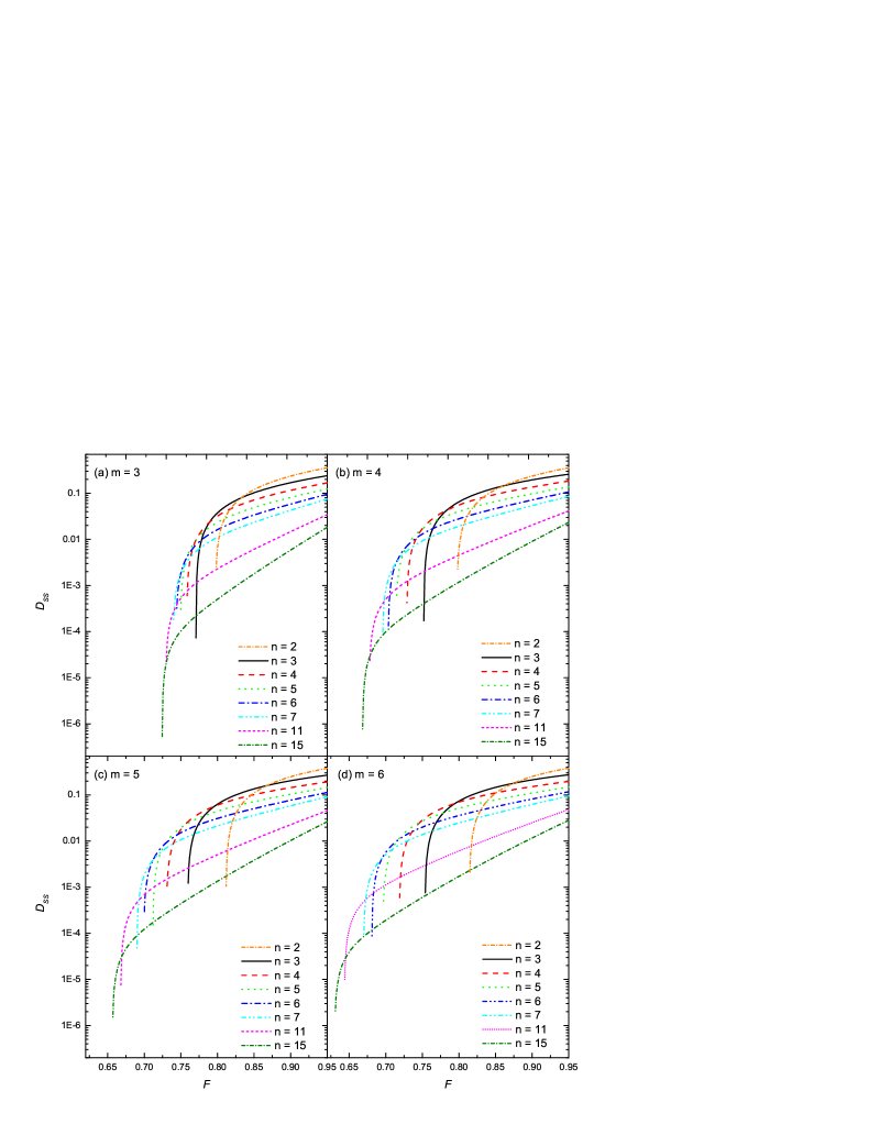
Figure 2: The yield $D_{\textrm{SS}}$ of our first protocol for distilling $\left|\Phi^{m+}\right\rangle$ after passing through a depolarizing channel of fidelity $F$ using the classical repetition code $[n,1,n]$ as the inner code for various $n$ when (a) $m=2$, (b) $m=3$, (c) $m=4$ and (d) $m=5$.

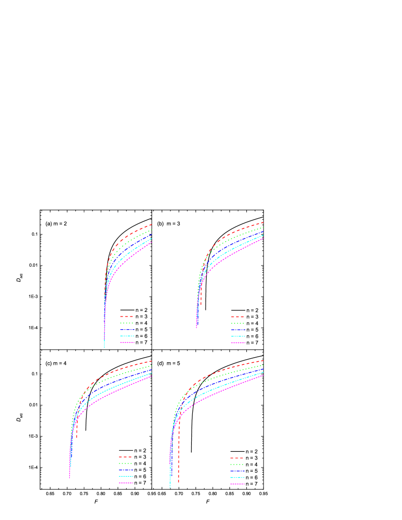
Figure 3: The yield $D_{\textrm{MS}}$ of our second protocol using the same sets of parameters as in Fig. 2.

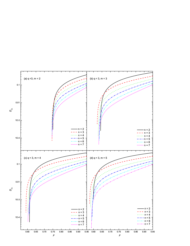
Figure 4: The yield $D_{\textrm{CL}}$ of our third protocol using the same sets of parameters as in Fig. 2.

Our numerical computation shows that $\lim_{n\rightarrow\infty}F_{\text{min}}^{\textrm{SS}}(m,n)$, $\lim_{n\rightarrow\infty}F_{\text{min}}^{\textrm{MS}}(m,n)$ and $\lim_{n\rightarrow\infty}F_{\text{min}}^{\textrm{CL}}(m,n)$ are decreasing functions of $m$. Besides, $\lim_{n\rightarrow\infty}F_{\text{min}}^{\textrm{SS}}(4,n)$ is smaller than 0.7798, the fidelity threshold of the Maneva and Smolin’s hashing scheme in the large $m$ limit Maneva and Smolin (2002). So, for $m\geq 3$, our three protocols all tolerate a higher noise level than all other one-way schemes known to date. Figs. 2–4 further depict that the yields of our protocols $D_{\textrm{SS}}$, $D_{\textrm{MS}}$ and $D_{\textrm{CL}}$ are very steep functions of $F$ around their corresponding threshold fidelities. Thus, a reasonable yield can be obtained when $F$ is equal to, say, $0.02$ higher than the threshold.

Another interesting feature found in Tables 2–4 and Figs. 2–4 is that the threshold fidelities $F_{\text{min}}^{\textrm{SS}}(m,n)$, $F_{\textrm{min}}^{\textrm{MS}}(m,n)$ and $F_{\textrm{min}}^{\textrm{CL}}(m,n)$ are all decreasing functions of $n$ for $m\geq 3$. That is, our protocols attain a higher capacity if players use a longer repetition code whenever $m\geq 3$. In contrast, DiVincenzo et al. found that $F_{\text{min}}^{\textrm{SS}}(2,n)$ attains global minimum when $n=5$. Besides, $F_{\text{min}}^{\textrm{SS}}(2,n)>F_{\text{min}}^{\textrm{SS}}(2,n\pm 1)$ for a small even integer $n$ DiVincenzo et al. (1998). Interestingly, Tables 3 and 4 show that $F_{\textrm{min}}^{\textrm{MS}}(2,n)$ and $F_{\textrm{min}}^{\textrm{CL}}(2,n)$ behave in the same way, too.

Lastly, we remark that for $m\geq 3$, the improvement in the error-tolerant capability for increasing $n$ comes with a price. For a fixed $m\geq 3$, the yields of our protocols decrease as $n$ increases provided that the channel fidelity $F$ is close to $1$ as depicted in Figs. 2–4. This is because as $n$ increases, more shared GHZ states must be wasted in order to obtain the error syndrome $\vec{\boldsymbol{s}}$ even if the channel is noiseless.

III.4 Understanding the trend of the threshold fidelities

Although the discussions in this subsection focuses on the trend of the threshold fidelity of our first protocol, namely, $F_{\textrm{min}}^{\textrm{SS}}(m,n)$, the essential ideas also apply to the cases of our second and third protocols, that is, $F_{\textrm{min}}^{\textrm{MS}}(m,n)$ and $F_{\textrm{min}}^{\textrm{CL}}(m,n)$.

The reason why $F_{\text{min}}^{\textrm{SS}}(2,n)$ is a sawtooth-shaped function of $n$ for $n\lesssim 8$ is related to the behavior of $h(\{\text{Pr}((\delta,\boldsymbol{\gamma})|\vec{\boldsymbol{s}}):(\delta,\boldsymbol{\gamma})\in GF(2)^{m}\})$. It is easy to check that for $m=2$, $h(\{\text{Pr}((\delta,\boldsymbol{\gamma})|\vec{\boldsymbol{s}}):(\delta,\boldsymbol{\gamma})\in GF(2)^{m}\})$ is equal to (much less than) $2$ provided that the depolarization weight $\text{wt}(\vec{\boldsymbol{s}})=n/2$ ($\text{wt}(\vec{\boldsymbol{s}})\neq n/2$). For a small even $n$, there is a non-negligible probability of finding $\vec{\boldsymbol{s}}$ with $\text{wt}(\vec{\boldsymbol{s}})=n/2$ so that the root of $S_{X}=1$ and hence the value of $F_{\text{min}}^{\textrm{SS}}$ are determined mainly by the summing only over those $\vec{\boldsymbol{s}}$’s with depolarization weight $0$ or $n/2$ in Eq. (41). In contrast, for a small odd $n$, all entropies in the R.H.S. of Eq. (41) are much less than $2$. Hence, the corresponding value of $F_{\text{min}}^{\textrm{SS}}(2,n)$ is lower than $F_{\text{min}}^{\textrm{SS}}(2,n\pm 1)$. In other words, the reason for $F_{\text{min}}^{\textrm{SS}}(2,n)>F_{\text{min}}^{\textrm{SS}}(2,n\pm 1)$ for a small even $n$ is that there is a non-negligible chance that exactly half of Bell states used by the inner repetition code have spin flip error so that players have absolutely no idea what kind of error the remaining unmeasured Bell state has experienced.

However, the situation is very different when $m\geq 3$. In this case, the condition for $h(\{\text{Pr}((\delta,\boldsymbol{\gamma})|\vec{\boldsymbol{s}}):(\delta,\boldsymbol{\gamma})\in GF(2)^{m}\})\geq 2$ is that one can find an integer $i$ such that $f_{\vec{\boldsymbol{s}}}(i)\geq 2$ and $f_{\vec{\boldsymbol{s}}}(j)=0$ for all $j<i$. More importantly, for a depolarizing channel with $F>1/2$, the probability $\text{Pr}(\vec{\boldsymbol{s}})$ of finding this kind of $\vec{\boldsymbol{s}}$ with $h(\{\text{Pr}((\delta,\boldsymbol{\gamma})|\vec{\boldsymbol{s}}):(\delta,\boldsymbol{\gamma})\in GF(2)^{m}\})\geq 2$ is much less than that in the situation of $m=2$. Thus, the contribution of terms with entropy greater than or equal to $2$ in Eq. (41) becomes much less significant when $m\geq 3$. So, it is not surprising to find that for a fixed $m\geq 3$, $F_{\text{min}}^{\textrm{SS}}(m,n)$ is not a sawtooth-shaped function of $n$ when $n$ is small.

It is also easy to understand why $\lim_{n\rightarrow\infty}F_{\text{min}}^{\textrm{SS}}(m,n)$ is a decreasing function of $m$. One simply check by Taylor’s series expansion that in the limit of large $n$ and for a fixed $1/2<F<1$. Then we find that the first term in the R.H.S. of Eq. (41) is an increasing function of $m$; and that the summand in the second term in the R.H.S. of Eq. (41) is almost surely a decreasing function of $m$ in the large $n$ limit.

As we have pointed out that the value of $F_{\text{min}}^{\textrm{SS}}(m,n)$ depends on the entropy of a few atypical set of errors experienced by the GHZ states. We do not have a good explanation why $F_{\text{min}}^{\textrm{SS}}(m,n)$ is a decreasing function of $n$ for $m\geq 3$.

III.5 Breaking the $F>0.75$ limit?

No $t$ error correcting quantum code of codeword size $4t$ exists Knill and Laflamme (1997); Bennett et al. (1996). Hence, it is impossible to distill Bell states using an one-way scheme provided that the fidelity of the depolarizing channel is less than or equal to $0.75$ Bennett et al. (1996). That is why $F_{\text{min}}^{\textrm{SS}}(2,n),F_{\textrm{min}}^{\textrm{MS}}(2,n),F_{\textrm{min}}^{\textrm{CL}}(2,n)>0.75$. Interestingly, a few $F_{\text{min}}^{\textrm{SS}}(m,n)$’s, $F_{\text{min}}^{\textrm{MS}}(m,n)$’s and $F_{\text{min}}^{\textrm{CL}}(m,n)$’s listed in Tables 2–4 are less than 0.75. Does it make sense?

To solve this paradox, let us recall that the Pauli errors experienced by a GHZ state shared among $m$ players can always be regarded as taken place in $(m-1)$ of the $m$ qubits. From Eq. (II.1), we may regard that at most one of the $(m-1)$ qubits may experience a phase error. So, the probability that a depolarized GHZ state has experienced phase error but not spin flip is $(1-F)/(2^{m}-1)$, where $F$ is the channel fidelity. And the number of erroneous qubits equals $1$ in this case. Besides, the probability that exactly $i$ out of the $(m-1)$ qubits have experienced spin flip is $2(1-F){m-1\choose i}/(2^{m}-1)$ for $i=1,2,\ldots,m-1$, where the extra factor of $2$ comes from the fact that the spin-flipped GHZ state may experience phase shift as well. Hence, the average number of erroneous qubits divided by $(m-1)$ is given by

$$\bar{e}=\frac{1}{m-1}\left[\frac{1-F}{2^{m}-1}+\frac{2(1-F)}{2^{m}-1}\sum_{i=1}^{m-1}i\enspace{m-1\choose i}\right]=\frac{1-F}{2^{m}-1}\left(2^{m-1}+\frac{1}{m-1}\right)~{}.$$ (42)

Since no $t$ error correcting quantum code has codeword size less than or equal to $4t$ Knill and Laflamme (1997); Bennett et al. (1996), $\bar{e}<1/4$. Consequently, a lower bound for the threshold fidelities $F_{\text{min}}^{\textrm{x}}(m,n)$ (for $\textrm{x}=\textrm{SS},\textrm{MS},\textrm{CL}$) is given by

$$F_{\text{min}}^{\textrm{x}}(m,n)>F_{\text{bound}}=1-\frac{2^{m}-1}{4}\left(2^{m-1}+\frac{1}{m-1}\right)^{-1}~{}.$$ (43)

A quick look at the third and the fourth columns in Table 1 convinces us that our protocols do not violate this general limit. Actually, one of the reasons why we can distill shared GHZ states when $F<0.75$ for $m\geq 3$ is that the average qubit error rate for a depolarized GHZ state is given by Eq. (42), which is smaller than $(1-F)$. Note in particular that in the large $m$ limit, the average qubit error rate for a depolarized GHZ state is close to $1/2$. So, it is not surprising that the bound $F_{\text{bound}}$ approaches $1/2$ in this case.

IV Generalization to higher dimensional spin

IV.1 Our extended protocols

Our three protocols can be generalized to the case when the Hilbert space dimension of each quantum particle is greater than 2. That is to say, the $m$ players wanted to share the state

$$\left|\Phi^{m+}_{q}\right\rangle=\frac{1}{\sqrt{q}}\sum_{i=0}^{q-1}\left|i^{\otimes m}\right\rangle$$ (44)

through a depolarizing channel by one-way entanglement distillation. The quantum codes used in the three generalized protocols are extensions of their corresponding binary codes to the $q$-nary ones. In particular, their common inner code becomes classical $[n,1,n]_{q}$ repetition code.

We have the following two cases to consider.

1. For $q=p^{m}$ where $p$ is a prime number, we may impose a finite field structure $GF(q)$ to the system by defining

   $$X_{j}:\left|i\right\rangle\longmapsto\left|i+j\right\rangle$$ (45)

   and

   $$Z_{j}:\left|i\right\rangle\longmapsto\omega_{p}^{\mathrm{Tr}{(ij)}}\left|i\right\rangle$$ (46)

   for all $j\in GF(q)$ where $\omega_{p}$ is a primitive $p$th root of unity, $\mathrm{Tr}$ is the absolute trace and all arithmetic are performed in the finite field $GF(q)$.

2. Alternatively, for any integer $q\geq 2$, we may impose a ring structure ${\mathbb{Z}}/q{\mathbb{Z}}$ to the system by defining

   $$X_{j}:\left|i\right\rangle\longmapsto\left|i+j\right\rangle$$ (47)

   and

   $$Z_{j}:\left|i\right\rangle\longmapsto\omega_{q}^{ij}\left|i\right\rangle$$ (48)

   for all $j\in\mathbb{Z}/q\mathbb{Z}$ where $\omega_{q}$ is a primitive $q$th root of unity and all arithmetic are performed in the ring ${\mathbb{Z}}/q{\mathbb{Z}}$.

From now on, we use the symbol ${\mathbb{K}}$ to denote either the finite field $GF(q)$ or the ring ${\mathbb{Z}}/q{\mathbb{Z}}$. Similar to the case of $q=2$, we use the compact notation $(\beta,\boldsymbol{\alpha})\equiv(\beta,\alpha_{1},\alpha_{2},\ldots,\alpha_{m-1})$ to denote the eigenvalue of the stabilizer generators where $\beta\in{\mathbb{K}}$ and $\boldsymbol{\alpha}\in{\mathbb{K}}^{m-1}$.

In the qubit case (that is, $q=2$), the error syndrome measurement is performed with the aid of CNOT gates. In the case of $q>2$, this can be done via the operator $|i,j\rangle\longrightarrow|i,i-j\rangle$ for all $i,j\in{\mathbb{K}}$. Suppose the error experienced by the $j$th copy of $\left|\Phi^{m+}_{q}\right\rangle$ is $(\beta_{j},\boldsymbol{\alpha}_{j})$ for $j=0,\ldots,n-1$. Then after measuring the error syndrome for the classical $[n,1,n]_{q}$ repetition code, we get $\vec{\boldsymbol{s}}\equiv(\boldsymbol{s}_{1},\ldots,\boldsymbol{s}_{n-1})$ where

$$\boldsymbol{s}_{j}\equiv\boldsymbol{\alpha}_{j}-\boldsymbol{\alpha}_{0}$$ (49)

for $1\leq j\leq n-1$. Furthermore, the remaining state shared among the players becomes

$$(\delta,\boldsymbol{\gamma})=(\sum_{j=0}^{n-1}\beta_{j},\boldsymbol{\alpha}_{0})~{}.$$ (50)

IV.2 Finding the capacities of our three generalized protocols

The analysis in Sec. III.2 can be easily generalized to the case of qudits (that is, $q>3$). In particular, we prove in the Appendix that

$$\text{Pr}((\delta,\boldsymbol{\gamma})|\vec{\boldsymbol{s}})=\left\{\begin{array}[]{ll}\displaystyle\frac{q^{k-1}(1-F)^{k}(q^{m}F-qF+q-1)^{n-k}}{\sum_{i}f_{\vec{\boldsymbol{s}}}(i)\left[q(1-F)\right]^{i}\left(q^{m}F-qF+q-1\right)^{n-i}}&\enspace\text{if}\enspace k>0,\\ \\ \displaystyle\frac{(q^{m}F-qF+q-1)^{n}+(q-1)\left(q^{m}F-1\right)^{n}}{q\sum_{i}f_{\vec{\boldsymbol{s}}}(i)\left[q(1-F)\right]^{i}\left(q^{m}F-qF+q-1\right)^{n-i}}&\enspace\text{if}\enspace k=0\enspace\text{and}\enspace\delta=0,\\ \\ \displaystyle\frac{(q^{m}F-qF+q-1)^{n}-\left(q^{m}F-1\right)^{n}}{q\sum_{i}f_{\vec{\boldsymbol{s}}}(i)\left[q(1-F)\right]^{i}\left(q^{m}F-qF+q-1\right)^{n-i}}&\enspace\text{if}\enspace k=0\enspace\text{and}\enspace\delta\neq 0,\end{array}\right.$$ (51)

where $k$ and $f_{\vec{\boldsymbol{s}}}(i)$ are given by Eq. (30) and Eq. (61) respectively.

The yields of our three generalized protocols can be computed using Eqs. (8)–(9) and (13)–(17) just like the case of $q=2$. Nevertheless, there is an important subtlety. Since the players can make full use of each of the $q$ possible error syndrome measurement outcomes to distill the generalized GHZ state $|\Phi_{q}^{m+}\rangle$, the entropies and conditional entropies in Eqs. (9), (14), (15) and (17) should be measured in the unit of dit rather than bit. That is to say, the base of the logarithm used in these entropies should be $q$ instead of $2$. And since the dimension of each information carrier $q$ has changed, one should not directly compare the yields of the qudit-based protocols with those of the standard qubit-based ones. Note further that similar to the original qubit-based protocols, we can compute these yields in a time sub-exponential in $n$.

IV.3 Performance of our generalized protocols

Figs. 5–7 depict the yields of our three generalized protocols in the case of $q=3$. And Tables 5–7 list the corresponding threshold fidelities. Clearly, the trend of the threshold fidelities of our three generalized protocols are very similar to their corresponding cases of $q=2$. In particular, for $q=3$, the threshold fidelities $F_{\textrm{min}}^{\textrm{SS}}(m,n)$, $F_{\textrm{min}}^{\textrm{MS}}(m,n)$ and $F_{\textrm{min}}^{\textrm{CL}}(m,n)$ are decreasing function of $n$ for any fixed integer $m\geq 3$; while they reach global minima at $n=7$ provided that $m=2$. These findings are not completely surprising because the arguments we have used to explain the trends of the yields and threshold fidelities for our three protocols in the case of $q=2$ reported in Sec. III.4 are also applicable here after minor adjustments.

		$m$
$F_{\textrm{min}}(m,n)$		2		3		4		5		6
	2	0.7462		0.7538		0.7609		0.7693		0.7778
	3	0.7445		0.7243		0.7145		0.7127		0.7148
	4	0.7445		0.7089		0.6885		0.6799		0.6779
$n$	5	0.7442		0.6994		0.6722		0.6588		0.6539
	6	0.7441		0.6927		0.6611		0.6443		0.6370
	7	0.7441		0.6877		0.6530		0.6337		0.6246
	11	0.7444		0.6759		0.6338		0.6096		0.5962
	15	0.7449		0.6700		0.6238		0.5974		0.5823

Table 5: The threshold fidelity $F_{\textrm{min}}^{\textrm{SS}}$ as a function of $m$ and $n$ for $q=3$.

		$m$
$F_{\textrm{min}}^{\textrm{MS}}(m,n)$		2		3		4		5		6
	2	0.7499		0.7114		0.6892		0.6780		0.6728
	3	0.7450		0.7034		0.6776		0.6640		0.6575
	4	0.7448		0.6944		0.6591		0.6389		0.6289
$n$	5	0.7444		0.6849		0.6452		0.6234		0.6127
	6	0.7443		0.6829		0.6418		0.6172		0.6041
	7	0.7443		0.6810		0.6390		0.6121		0.5967
	11	0.7446		0.6738		0.6289		0.5997		0.5808
	15	0.7451		0.6692		0.6212		0.5927		0.5740

Table 6: The threshold fidelity $F_{\textrm{min}}^{\textrm{MS}}$ as a function of $m$ and $n$ for $q=3$.

		$m$
$F_{\textrm{min}}^{\textrm{CL}}(m,n)$		2		3		4		5		6
	2	0.7499		0.6419		0.6120		0.5981		0.5921
	3	0.7450		0.6222		0.5908		0.5762		0.5697
	4	0.7448		0.6282		0.6016		0.5821		0.5868
$n$	5	0.7444		0.6337		0.6104		0.5916		0.5895
	6	0.7443		0.6334		0.6061		0.5896		0.5855
	7	0.7443		0.6304		0.6023		0.5877		0.5829
	11	0.7446		0.6249		0.5910		0.5790		0.5670
	15	0.7451		0.6235		0.5865		0.5701		0.5560

Table 7: The threshold fidelity $F_{\textrm{min}}^{\textrm{CL}}$ as a function of $m$ and $n$ for $q=3$.

Figure 5: The yield $D_{\textrm{SS}}$ of our first generalized protocol for distilling $\left|\Phi^{m+}_{3}\right\rangle$ after passing through a depolarizing channel of fidelity $F$ using the classical repetition code $[n,1,n]_{q}$ as the inner code for various $n$ when (a) $m=2$, (b) $m=3$, (c) $m=4$ and (d) $m=5$.

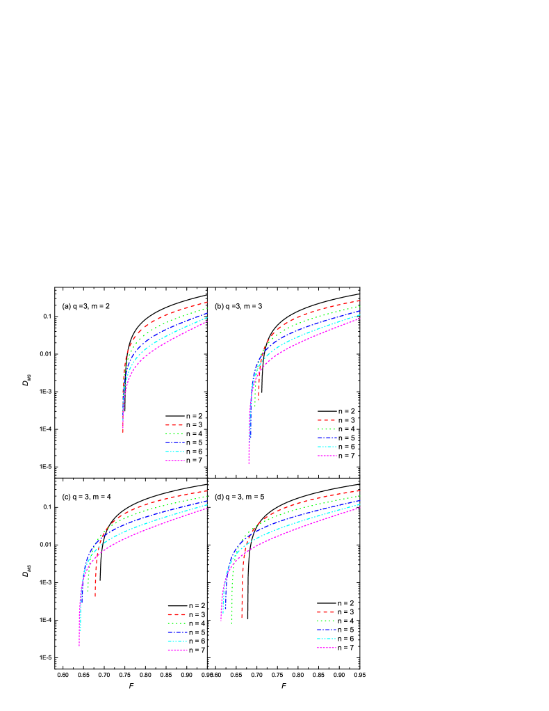
Figure 6: The yield $D_{\textrm{MS}}$ of our second generalized protocol for distilling $\left|\Phi^{m+}_{3}\right\rangle$. The parameters used are the same as those in Fig. 5.

Figure 7: The yield $D_{\textrm{CL}}$ of our third generalized protocol for distilling $\left|\Phi^{m+}_{3}\right\rangle$. The parameters used are the same as those in Fig. 5.

IV.4 Lower bound for the three threshold fidelities

The proof that no $t$ error correcting quantum code with codeword size $4t$ is also applicable to qudits Rains (1999). We may use this fact to establish a lower bound for the threshold fidelities of our three generalized protocols when qudits are used as information carriers. Since the proof is also the same as that of the qubit case reported in Sec. III.5, here we only write down the bound without giving the details of the proof:

$$F_{\text{min}}^{\textrm{SS}}(m,n),F_{\text{min}}^{\textrm{MS}}(m,n),F_{\text{min}}^{\textrm{CL}}(m,n)>F_{\text{bound}}=1-\frac{q^{m}-1}{4(q-1)}\left(q^{m-1}+\frac{1}{m-1}\right)^{-1}~{}.$$ (52)

V Summary and Discussion

In summary, we have introduced three one-way GHZ state purification protocols using degenerate codes by extending the works of DiVincenzo et al. on one-way Bell state purification via degenerate codes Shor and Smolin (1996); DiVincenzo et al. (1998) as well as the works of Maneva and Shor Maneva and Smolin (2002) and its generalization by Chen and Lo Chen and Lo (2007) on multipartite entanglement purification using random asymmetric CSS codes. Then, we calculate the yields of our three protocols when the inputs are Werner states. The method we used to calculate these yields is divided into two steps. The first step is to calculate entropies or conditional entropies such as $h(\{\textrm{Pr}((\delta,\boldsymbol{\gamma}):(\delta,\boldsymbol{\gamma})\in GF(2)^{m}\})$ by means of the so-called depolarization weight enumerator. Actually, the first step can be easily extended to the case of an arbitrary stabilizer inner code, an arbitrary un-correlated noise model and an arbitrary stabilizer output state. The second step involves the computation of a weighted sum of the entropies or conditional entropies obtained in the first step. Nonetheless, for a general stabilizer inner code, a general un-correlated noise model and a general output state, this sum may not be practical as it involves up to about $2^{mn}$ number of terms. Fortunately, as the inner code used in our purification scheme is the highly symmetrical classical repetition code, we are able to greatly simplify the sum, making the computation of the yields in a time which is sub-exponential in $n$ when the GHZ states are subjected to depolarization errors. In this way, we can calculate the corresponding threshold fidelities accurately and reasonably fast. This is quite an accomplishment because finding the threshold fidelities involves the accurate determination of the sign of the difference between two small positive numbers provided that the number of players $m\geq 3$ and the codeword size of the inner repetition code $n$ is large. (See, for example, Eq. (41).) Just like the Bell state case, we discover that the threshold fidelities of our three protocols are better than all known one-way GHZ state purification schemes to date. So, once again, the power of using degenerate codes to combat quantum errors is demonstrated.

We also extended our scheme to tackle the case when the information carriers are qudits instead of qubits. We find that the performance trend of these generalized schemes are quite similar to those of the qubit cases.

There are a few un-answered questions, however. Here we list some of them. The reason why the threshold fidelities $F_{\text{min}}^{\textrm{SS}}$ $F_{\textrm{min}}^{\textrm{MS}}$ and $F_{\textrm{min}}^{\textrm{CL}}$ decrease with $n$ for $m\geq 3$ is not apparent. And apart from the general statement that degenerate codes pack more information than non-degenerate ones making them powerful in one-way purification of GHZ states, can we specifically understand why using classical repetition code concatenated with a random hashing quantum code is more error-tolerant than a few other choices of degenerate codes? Ho and Chau (2008) Along a different line, it is important to find out the value of $\lim_{m\rightarrow\infty}\lim_{n\rightarrow\infty}F_{\text{min}}^{\textrm{CL}}(m,n)$ and compare it with the $1/2$ lower bound. Finally, it is instructive to extend our study to the case of using a different degenerate code to distill another type of entangled state subjected to another noise model, such as the Pauli channel Smith and Smolin (2007).

Appendix A Proof Of Eq. (51)

We prove the validity of Eq. (51) by following the analysis in Sec. III.2. (And we follow the same notations as used in Sec. III.2 after possibly some straight-forward extension to the case of qudits.) First, we extend the definition of depolarization weight as follows. Let $(\beta_{j},\boldsymbol{\alpha}_{j})_{j=0}^{n-1}\in{\mathbb{K}}^{mn}$ be a ordered $n$-tuple. Then its depolarization weight is defined as the Hamming weight by regarding this $n$-tuple as a vector of elements in ${\mathbb{K}}$. Clearly, $\text{Pr}((\delta,\boldsymbol{\gamma})\wedge\vec{\boldsymbol{s}})=\text{Pr}({\mathfrak{E}}(\vec{\boldsymbol{s}},\delta,\boldsymbol{\gamma}))$ where

$${\mathfrak{E}}(\vec{\boldsymbol{s}},\delta,\boldsymbol{\gamma})=\{(\beta_{j},\boldsymbol{\alpha}_{j})_{j=0}^{n-1}\in{\mathbb{K}}^{mn}:\delta=\sum_{j=0}^{n-1}\beta_{j},\boldsymbol{\gamma}=\boldsymbol{\alpha}_{0},\boldsymbol{\alpha}_{\ell}=\boldsymbol{s}_{\ell}+\boldsymbol{\alpha}_{0}\enspace\text{for}\enspace\ell=1,2,\ldots,n-1\}~{}.$$ (53)

Using the same argument as in the case of $q=2$, we conclude that for $k>0$,

$$w({\mathfrak{E}}(\vec{\boldsymbol{s}},\delta,\boldsymbol{\gamma});x,y) = \frac{1}{q}\sum_{\{a_{i,\boldsymbol{t}}\}}\frac{k!}{\displaystyle\prod_{\genfrac{}{}{0.0pt}{}{i\in{\mathbb{K}},}{\boldsymbol{t}\in{{\mathbb{K}}^{m-1}}\setminus\{\boldsymbol{0}\}}}a_{i,\boldsymbol{t}}!}\enspace\frac{(n-k)!}{\displaystyle\prod_{i\in{\mathbb{K}}^{*}}a_{i,\boldsymbol{0}}!}\enspace x^{n-a_{0,\boldsymbol{0}}}y^{a_{0,\boldsymbol{0}}}$$ (54)

$$= q^{k-1}\sum_{a_{0,\boldsymbol{0}}}{n-k\choose a_{0,\boldsymbol{0}}}\enspace(q-1)^{n-k-a_{0,\boldsymbol{0}}}x^{n-a_{0,\boldsymbol{0}}}y^{a_{0,\boldsymbol{0}}}$$

$$= q^{k-1}x^{k}[(q-1)x+y]^{n-k}~{}.$$

For $k=0$, we have to use a slightly different method to compute the depolarization weight enumerator. By substituting $x_{0}=y$ and $x_{\eta}=x$ for all $\eta\neq 0$ into the identity

$$\left(\sum_{\eta\in{\mathbb{K}}}x_{\eta}\right)^{n}=\sum_{\{a_{\eta}\}}\left(\frac{n!}{\prod_{\eta\in{\mathbb{K}}}a_{\eta}!}\prod_{\eta\in{\mathbb{K}}}x_{\eta}^{a_{\eta}}\right)~{},$$ (55)

we have

$$\sum_{\delta\in{\mathbb{K}}}w({\mathfrak{E}}(\vec{\boldsymbol{s}},\delta,\boldsymbol{\gamma});x,y)=[(q-1)x+y]^{n}~{}.$$ (56)

If ${\mathbb{K}}=GF(q)$, then by putting $x_{0}=y$ and $x_{\eta}=\omega_{p}^{\mathrm{Tr}(\eta\rho)}x$ for all $\eta\neq 0$ where $\rho\in GF(q)^{*}$ into Eq. (55), we have

$$\sum_{\delta\in GF(q)}\omega_{p}^{\mathrm{Tr}(\delta\rho)}w({\mathfrak{E}}(\vec{\boldsymbol{s}},\delta,\boldsymbol{\gamma});x,y)=(y-x)^{n}~{}.$$ (57)

If ${\mathbb{K}}={\mathbb{Z}}/q{\mathbb{Z}}$, then we put $x_{0}=y$ and $x_{\eta}=\omega_{q}^{\eta\rho)}x$ for all $\eta\neq 0$ where $\rho\in({\mathbb{Z}}/q{\mathbb{Z}})^{*}$ into Eq. (55), we arrive at

$$\sum_{\delta\in{\mathbb{Z}}/q{\mathbb{Z}}}\omega_{q}^{\delta\rho}w({\mathfrak{E}}(\vec{\boldsymbol{s}},\delta,\boldsymbol{\gamma});x,y)=(y-x)^{n}~{}.$$ (58)

Consequently, we conclude that for ${\mathbb{K}}=GF(q)$ or ${\mathbb{Z}}/q{\mathbb{Z}}$,

$$w({\mathfrak{E}}(\vec{\boldsymbol{s}},\delta,\boldsymbol{\gamma});x,y)=\left\{\begin{array}[]{ll}\displaystyle q^{k-1}x^{k}\left[(q-1)x+y\right]^{n-k}&\enspace\text{if}\enspace k>0,\\ \\ \displaystyle\frac{1}{q}\left\{\left[(q-1)x+y\right]^{n}+(q-1)(y-x)^{n}\right\}&\enspace\text{if}\enspace k=0\enspace\text{and}\enspace\delta=0,\\ \\ \displaystyle\frac{1}{q}\left\{\left[(q-1)x+y\right]^{n}-(y-x)^{n}\right\}&\enspace\text{if}\enspace k=0\enspace\text{and}\enspace\delta\neq 0.\end{array}\right.$$ (59)

Surely, for depolarizing channel, $\text{Pr}((\delta,\boldsymbol{\gamma})\wedge\vec{\boldsymbol{s}})=w({\mathfrak{E}}(\vec{\boldsymbol{s}},\delta,\boldsymbol{\gamma});(1-F)/(q^{m}-1),F)$ and

$$\text{Pr}(\vec{\boldsymbol{s}}) = \sum_{\boldsymbol{t}}\left[\frac{q(1-F)}{q^{m}-1}\right]^{k(\vec{\boldsymbol{s}},\boldsymbol{t})}\left[F+\frac{(q-1)(1-F)}{q^{m}-1}\right]^{n-k(\vec{\boldsymbol{s}},\boldsymbol{t})}$$ (60)

$$= \frac{1}{(q^{m}-1)^{n}}\sum_{i=0}^{n}f_{\vec{\boldsymbol{s}}}(i)\left[q(1-F)\right]^{i}\left(q^{m}F-qF+q-1\right)^{n-i}~{},$$

where

$$f_{\vec{\boldsymbol{s}}}(i)=|\{\boldsymbol{t}\in{\mathbb{K}}^{m-1}:k(\vec{\boldsymbol{s}},\boldsymbol{t})=i\}|~{}.$$ (61)

Combining Eqs. (59)–(61), we arrive at Eq. (51). $\Box$

References

- Shor and Smolin (1996) P. W. Shor and J. A. Smolin, quant-ph/9604006v2 (1996).
- DiVincenzo et al. (1998) D. P. DiVincenzo, P. W. Shor, and J. A. Smolin, Phys. Rev. A 57, 830 (1998).
- Dür et al. (1999) W. Dür, J. I. Cirac, and R. Tarrach, Phys. Rev. Lett. 83, 3562 (1999).
- Maneva and Smolin (2002) E. N. Maneva and J. A. Smolin, AMS Contemporary Mathematics Series 305, 203 (2002).
- Bennett et al. (1996) C. H. Bennett, D. P. DiVincenzo, J. A. Smolin, and W. K. Wootters, Phys. Rev. A 54, 3824 (1996).
- Chen and Lo (2007) K. Chen and H.-K. Lo, Quant. Inf. & Comp. 7, 689 (2007).
- Hostens et al. (2006a) E. Hostens, J. Dehaene, and B. DeMoor, Phys. Rev. A 73, 042316 (2006a).
- Hostens et al. (2006b) E. Hostens, J. Dehaene, and B. DeMoor, Phys. Rev. A 74, 062318 (2006b).
- Kay et al. (2006) A. Kay, J. K. Pachos, W. Dür, and H.-J. Briegel, New J. Phys. 8, 147 (2006).
- Goyal et al. (2006) K. Goyal, A. McCauley, and R. Raussendorf, Phys. Rev. A 74, 032318 (2006).
- Glancy et al. (2006) S. Glancy, E. Knill, and H. M. Vasconcelos, Phys. Rev. A 74, 032319 (2006).
- Andrews (1976) G. E. Andrews, The Theory Of Partitions (Addison-Wesley, Reading, MA, 1976), Eq. (5.1.2) in p. 70.
- Knill and Laflamme (1997) E. Knill and R. Laflamme, Phys. Rev. A 55, 900 (1997).
- Rains (1999) E. Rains, IEEE Trans. Info. Theory 45, 1827 (1999).
- Ho and Chau (2008) K. H. Ho and H. F. Chau, unpublished (2008).
- Smith and Smolin (2007) G. Smith and J. A. Smolin, Phys. Rev. Lett. 98, 030501 (2007).