Domain wall motion of magnetic nanowires under a static field
Abstract
The propagation of a head-to-head magnetic domain-wall (DW) or a tail-to-tail DW in a magnetic nanowire under a static field along the wire axis is studied. Relationship between the DW velocity and DW structure is obtained from the energy consideration. The role of the energy dissipation in the field-driven DW motion is clarified. Namely, a field can only drive a domain-wall propagating along the field direction through the mediation of a damping. Without the damping, DW cannot propagate along the wire. Contrary to the common wisdom, DW velocity is, in general, proportional to the energy dissipation rate, and one needs to find a way to enhance the energy dissipation in order to increase the propagation speed. The theory provides also a nature explanation of the wire-width dependence of the DW velocity and velocity oscillation beyond Walker breakdown field.
pacs:
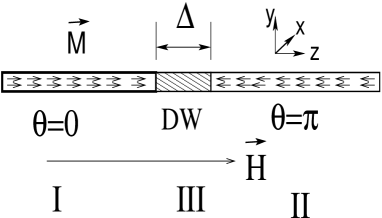
75.60.Jk, 75.60.Ch, 85.70.Kh, 74.25.HaManipulation of domain wall (DW) of magnetic nanowires by a fieldOno ; Cowburn ; Erskine ; Parkin1 ; Erskine1 and/or by a currentErskine1 ; Ber ; Thia ; Mae ; Klaui ; Parkin2 has recently attracted much attention because of its academic interest and potential applications in information storageParkin . Many interesting phenomena were discovered with limited understandings. For a tail-to-tail DW or a head-to-head DW as shown in Fig. 1 in a magnetic nanowire with its easy-axis along the wire axis, the DW will propagate in the wire under an external magnetic field parallel to the wire axis or a current through the wire. The propagating speed of the DW depends on the field strengthErskine ; Parkin1 and/or the current densityErskine1 ; Parkin2 . For the field-driven DW motion, there exists a so-called Walker’s breakdown field Walker . The DW velocity is proportional to the external field for and . DW velocity decreases as the field increases between the two linear H-dependence regimes. The linear regimes are characterized by the DW mobility . For , the DW velocity may also oscillate with timeWalker ; Erskine . Experiments also found that the DW velocity is sensitive to both DW structures and wire widthOno ; Cowburn ; Erskine . Magnetization dynamics is governed by a nonlinear differential equation, called Landau-Lifschitz-Gilbert (LLG) equation. Spatial homogeneous solutions of this equation related to the optimal magnetization reversal of Stoner particles may be solved analyticallyxrw , but general solutions for the DW motion are not known. Our current theoretical knowledge about DW motion is either from the seminar work of WalkerWalker or from the Slonczewski’s one-dimensional modelSlon in which a DW is treated as a rigid body characterized by DW position and a cant angle from the demagnetic field of a film. Both theories are developed for one-dimensional transverse DW of a uniaxial magnetic wire with a demagnetic field.
Though much progress have been made on both experimental and theoretical aspects, DW motion is still poorly understood. Slonczewski model is a great simplification of DW motion from the LLG equation. This model does not contain the detail structure of DW with DW width as an input parameter. Thus the theory can explain neither DW velocity oscillation nor many other interesting issues. Walker’s theory is based on a particular solution of the LLG equation in a special case that does not distinguish different types of DWs. It predicts that the DW mobility is proportional to the DW width and inversely proportional to the damping constant, , where is gyromagnetic ratio, is the DW width and is damping constant. Walker’s analytical analysis is useful in understanding some aspects of experimental findings, but it does not provide deep insight into DW motion such as the origin of the motion. In fact, Walker’s expression of the DW mobility is strange because it is singular in . It does not tell us what will happen when damping goes to zero (the limit of does not exist, and the limit of depends on that is a numeric number smaller than 1). Although Walker’s solution is only correct for a strictly one-dimensional uniaxial wire with a demagnetic field and there is no proof of its correctness for other types of wires, it was widely used to understand DW motion. Thus, it is important to prove whether is true for an arbitrary magnetic wire and to know how the result should be modified if it is not.
In this letter, we shall examine the field-induced DW propagation from an angle different from those of Walker and Slonczewski. Firstly, we shall, from a simple model calculation, show that no static head-to-head DWs or tail-to-tail DWs are allowed in the presence of an external magnetic field along the wire axis. Secondly, energy conservation principle prevents a DW from propagating in the absence of a damping even under a static field, and it leads to a general relationship between the DW velocity and DW structure. Contrary to the common wisdom, DW velocity is proportional to the energy dissipation rate. Thus, the intrinsic critical field for DW propagation in a wire is zero, and the DW velocity is in general proportional to damping constant. Finally, our theory can reproduce the results of both Walker’s and Slonczewski’s models. Furthermore, the present theory attributes a DW velocity oscillation for to the periodic motion of the DW, either the precession of the DW or oscillation of the DW width.
In a magnetic material, magnetic domains are formed in order to minimize the stray field energy. A DW that separates two domains is defined by the balance between the exchange energy and the magnetic anisotropy energy. The stray field plays little role in a DW structure. To describe a head-to-head DW in a magnetic nanowire, let us consider a wire with its easy-axis along the wire axis (the shape anisotropy dominates other magnetic anisotropies and makes the easy-axis along the wire when the wire is small enough) which is chosen as the z-axis as illustrated in Fig. 1. Since the magnitude of the magnetization does not change in the LLG equationxrw , the magnetic state of the wire can be conveniently described by the polar angle (angle between and the z-axis) and the azimuthal angle . The magnetization energy is mainly from the exchange energy and the magnetic anisotropy because the stray field energy is negligible in this case. The wire energy can be written in general as
| (1) |
where is the energy density due to all kinds of magnetic anisotropies which has two equal minima at and (), term is the exchange energy, is the magnitude of magnetization, and is the external magnetic field along z-axis. In the absence of , a head-to-head static DW that separates domain from domain (Fig. 1) can exist in the wire. The domain structure is determined by the equations
| (2) |
In order to show that no intrinsic static head-to-head DW is allowed in the presence of an external field (), consider a special case that the wire is 1D and is a function of only. Then Eq. (2) should include the external field and becomes
| (3) |
The second equation requires . Since and or on the both sides of the DW, . Thus, one can multiply the first equation by and the integration of the first equation yields . However, for a head-to-head DW as shown in Fig. 1, in the far left is not compatible with in the far right. Thus, Eq. (3) does not have a head-to-head DW solution for . In other words, a DW in a nanowire under an external field must be time dependent that could be either a local motion or a propagation along the wire. It should be clear that above argument is only true for an intrinsic head-to-head DW, and it shall fail with defect pinning that changes Eq. (3). Indeed static DWs exist in the presence of a weak field in reality because of pinning.
The following results are based on the fact that a static field can be neither an energy source nor an energy sink. Without a damping, the system is a Hamiltonian system, and will move on an equal energy contour by energy conservation. This viewpoint was important in understanding magnetization reversal of Stoner particles in a static fieldxrw1 , and its extension was used to develop new strategiesxrw2 for the magnetization reversal of Stoner particles. From the LLG equationxrw1 , one can show that the energy damping rate is
| (4) |
where is the effective field. In regions I and II or inside a static DW, is parallel to . Thus no energy dissipation is possible there. The energy dissipation can only occur in the DW region when is not parallel to .
The total energy of the wire equals the sum of the energies of regions I, II, and III, . increases while decreases when the DW propagate from left to the right along the wire. The net energy change in region I plus II due to the DW propagation is
| (5) |
where is the DW propagating speed, and is the cross section of the wire. The energy of region III should not change much because the DW width is defined by the balance of exchange energy and magnetic anisotropy, and is usually order of . A DW cannot absorb or release too much energy, and can at most adjust temporarily energy dissipation rate. In other words, is either zero or fluctuates between positive and negative values with zero time-average. Since energy release from the magnetic wire should be equal to the energy dissipated (to the environment), one has
| (6) |
Thus, the relationship between the DW velocity and the DW structure is
| (7) |
where is the unit vector of . Eq. (7) is our central result. Obviously, the right side of this equation is fully determined by the DW structure. Time averaged velocity is
| (8) |
where bar denotes time average.
Because there is no intrinsic static head-to-head DWs in the presence of a static field, the first term in the right side of Eq. (7) will be positive and non-zero since a time dependent DW requires . Thus time-averaged is always positive. It implies zero intrinsic critical-field for DW propagation which is consistent with Walker’s resultWalker . A DW can have two possible types of motion under an external magnetic field. One is that a DW behaves like a rigid body propagating along the wire. This is the basic assumption in Slonczewski modelSlon ; Thia and Walker’s solution for . Obviously, DW energy is time-independent, . The other one is that the DW structure varies with time while it propagates in the wire. It means that the snap-shots of the DW at different time are different. In the first type of motion, if the DW keep its static structure in the absence of the external field, then the first term in the right side of Eq. (7) shall be proportional to , where , characterize the DW structure, is a numerical number of order of 1 (smaller than 1). This is because the effective field due to the exchange energy and magnetic anisotropy is parallel to , and does not contribute to the energy dissipation. Thus, in this case, with . To show that depends on material parameters, let us consider the Walker’sWalker model in which here and measure the magnetic anisotropies along the easy and hard axes, respectively. From Walker’s trial function
| (9) |
where is the DW width , Eq. (4) becomes
| (10) |
and DW energy change rate is
| (11) |
Substituting Eqs. (10) and (11) into Eq. (7), and together with Walker’s conjectures of and , one can easily reproduce Walker’s DW velocity expression for both and . For example, for , and Eq. (7) gives
| (12) |
This velocity expression is the same as that of the Slonczewski modelSlon ; Thia in a one-dimensional wire. In Walker’s analysis, is fixed by and through . Using this in the above velocity expression, Walker’s mobility coefficient is recovered. This inverse damping relation is from the particular potential landscape in -direction. One should expect different result if the shape of the potential landscape is changed. Thus, this expression should not be used to extract the damping constantOno ; Erskine .
A DW may be substantially distorted from its static structure when as it was revealed in Walker’s analysis. Generally speaking, a physical system under a constant driving force will first try a fixed point solutionxrw3 . It will go to other types of more complicated solutions only if a fixed point solution is not possible. In terms of DW motion, a domain wall will arrange itself as much as possible to satisfy Eq. (3). Of course, it is known that a head-to-head DW solution is only possible for Eq. (2) but not for Eq. (3). Thus, one should expect that is almost parallel to except a small perpendicular component of order of . One may assume with much smaller than 1. This assumption agrees with the minimum energy dissipation principleMea since when for is used, and any modification of should only make smaller. The DW propagating speed is then , a linear relation in both and , but a smaller DW mobility because of the smallness of . This smaller mobility at leads naturally to a negative differential mobility between and ! In other words, this negative differential mobility is due to the transition of the DW from a high energy dissipation structure to a lower one. This picture tells us that one should try to make a DW capable of dissipating as much energy as possible if one wants to achieve a high DW velocity. This is very different from what people would believe from Walker’s special mobility formula of inverse proportion of the damping constant. To increase the energy dissipation, one may reduce defects and surface roughness other than increasing the damping constant. The reason is, by minimum energy dissipation principle, that defects are extra freedoms to lower because, in the worst case, defects will not change when without defects are used.
In the case that the DW precess around wire axis or DW width breathes periodically or both motion are present, one should expect both and energy dissipation rate oscillate with time. According to Eq. (7), DW velocity will also oscillate. DW velocity should oscillate periodically if only one type of DW motion (precession or DW breathing) presents, but it could be very irregular if both motions are present and the ratio of their periods is irrational. Indeed, this oscillation was observed in a recent experimentErskine . It should be pointed out that the DW precession motion was already detected experimentally by MOKE broadening technologyErskine . How can one understand the wire-width dependence of the DW velocity? According to Eq. (7), the velocity is a functional function of DW structure which is very sensitive to the wire width. For example, for a very narrow wire, only transverse DW is possible while a vortex DW is preferred for a very wide wire (large than DW width). Different vortices yield different values of , which in turn results in different DW propagation speed.
The correctness of our central result Eq. (7) depends only on the LLG equation, the general energy expression of Eq. (1), and the fact that a static magnetic field can be neither an energy source nor an energy sink of a system. It does not depend on the details of a DW structure as long as the DW propagation is induced by a static magnetic field. In this sense, our result is very general and robust, and it is applicable to an arbitrary magnetic wire. However, it cannot be applied to a time-dependent field or the current-induced DW propagation, at least not directly. Also, it may be interesting to emphasize that there is no inertial in the DW motion within LLG description since this equation contains only the first order time derivative. Thus, there is no concept of mass in this formulation.
In conclusion, a global view of the field-induced DW propagation is provided, and the importance of energy dissipation in the DW propagation is revealed. A general relationship between the DW velocity and the DW structure is obtained. The result says: no damping, no DW propagation along a magnetic wire. It is shown that the intrinsic critical field for a head-to-head DW is zero. This zero intrinsic critical field is related to the absence of a static head-to-head DW in a magnetic field parallel to the nanowire. Thus, a non-zero critical field can only come from the pinning of defects or surface roughness. The observed negative differential mobility is due to the transition of a DW from a high energy dissipation structure to a low energy dissipation structure. Furthermore, the DW velocity oscillation is attributed to either the DW precession around wire axis or from the DW width oscillation.
This work is supported by Hong Kong UGC/CERG grants (# 603007 and SBI07/08.SC09).
References
- (1) T. Ono, H. Miyajima, K. Shigeto, K. Mibu, N. Hosoito, and T. Shinjo, Science 284, 468 (1999).
- (2) D. Atkinson, D.A. Allwood, G. Xiong, M.D. Cooke, C. Faulkner, and R.P. Cowburn, Nat. Mater. 2, 85 (2003).
- (3) G.S.D. Beach, C. Nistor, C. Knutson, M. Tsoi, and J.L. Erskine, Nat. Mater. 4, 741 (2005); J. Yang, C. Nistor, G.S.D. Beach, and J.L. Erskine, Phys. Rev. B 77, 014413 (2008).
- (4) M. Hayashi, L. Thomas, Y.B. Bazaliy, C. Rettner, R. Moriya, X. Jiang, and S.S.P. Parkin, Phys. Rev. Lett. 96, 197207 (2006).
- (5) G.S.D. Beach, C. Knutson, C. Nistor, M. Tsoi, and J.L. Erskine, Phys. Rev. Lett. 97, 057203 (2006).
- (6) L. Berger, Phys. Rev. B 73, 014407 (2006); ibid 75, 174401 (2007).
- (7) S. Zhang and Z. Li, Phys. Rev. Lett. 93, 127204 (2004); A. Thiaville, Y. Nakatani, J. Miltat, and Y. Suzuki, Europhys. Lett. 69, 990 (2005).
- (8) S.E. Barnes and S. Maekawu, Phys. Rev. Lett. 95, 107204 (2005).
- (9) M. Klaui, C.A.F. Vaz, J.A.C. Bland, W. Wernsdorfer, G. Faini, E. Cambril, L.J. Heyderman, F. Nolting, and U. Rudiger, Phys. Rev. Lett. 94, 106601 (2005).
- (10) L. Thomas, M. Hayashi, X. Jiang, R. Moriya, C. Rettner, and S.S.P. Parkin, Nature 443, 197 (2006); M. Hayashi, L. Thomas, C. Rettner, R. Moriya, Y.B. Bazaliy, and S.S.P. Parkin, Phys. Rev. Lett. 98, 037204 (2007).
- (11) S.S.P. Parkin, U.S. Patent No. US6834005 (2004).
- (12) N.L. Schryer and L.R. Walker, J. of Appl. Physics, 45, 5406 (1974).
- (13) D. Bouzidi and H. Suhl, Phys. Rev. Lett. 65, 2587 (1990).
- (14) Z.Z. Sun and X.R. Wang, Phys. Rev. Lett. 97, 077205 (2006); X.R. Wang and Z.Z. Sun, ibid 98, 077201 (2007).
- (15) A.P. Malozemoff and J.C. Slonczewski, Magnetic Domain Walls in Bubble Material (Academica, New York, 1979).
- (16) Z.Z. Sun, and X.R. Wang, Phys. Rev. B 71, 174430 (2005).
- (17) Z.Z. Sun, and X.R. Wang, Phys. Rev. B 73, 092416 (2006); 74 132401 (2006); T. Moriyama, R. Cao, J.Q. Xiao, J. Lu, X.R. Wang, Q. Wen, and H.W. Zhang, Appl. Phys. Lett. 90, 152503 (2007).
- (18) X. R. Wang, and Q. Niu, Phys. Rev. B 59, R12755 (1999); Z.Z. Sun, H.T. He, J.N. Wang, S.D. Wang, and X.R. Wang, Phys. Rev. B 69, 045315 (2004).
- (19) T. Sun, P. Meakin, and T. Jøssang, Phys. Rev. E 51, 5353 (1995).