A gauge invariant infrared stabilization of $3D$ Yang-Mills gauge theories

Abstract

We demonstrate that the inversion method can be a very useful tool in providing an infrared stabilization of $3D$ gauge theories, in combination with the mass operator $A^{2}$ in the Landau gauge. The numerical results will be unambiguous, since the corresponding theory is ultraviolet finite in dimensional regularization, making a renormalization scale or scheme obsolete. The proposed framework is argued to be gauge invariant, by showing that the nonlocal gauge invariant operator $A^{2}_{\min}$, which reduces to $A^{2}$ in the Landau gauge, could be treated in $3D$, in the sense that it is power counting renormalizable in any gauge. As a corollary of our analysis, we are able to identify a whole set of powercounting renormalizable nonlocal operators of dimension two.

LTH–782

1 Introduction

$3D$ gauge theories are not only of a pure theoretical importance. For example, they naturally appear as the very high temperature limit of their $4D$ counterpart [1], while $3D$ QED can be used as an effective theory describing high temperature cuprate superconductors [2].

When studying $3D$ gauge theories, a key observation is that the gauge coupling $g^{2}$ becomes a dimensionful quantity. A positive consequence is the ensuing superrenormalizability of $3D$ gauge theories, meaning that the ultraviolet sector is relatively well behaved. Unfortunately, this also inflicts a serious problem in the infrared [3]. A simple dimensional counting allows us to understand this problem intuitively. At consecutive orders in perturbation theory in the massive coupling $g^{2}$, an increasing number of inverse momenta is required to obtain a specific dimension of e.g. a particular Green function under study. Consequently, at increasing order of perturbation theory, the low momentum region becomes more and more divergent.

A natural solution to this problem might be the dynamical generation of a mass $m$, so that a perturbative expansion in the dimensionless parameter $\frac{g^{2}}{m}$ might emerge, ensuring a safe infrared limit. This has stimulated several studies, [4, 5, 6, 7, 8, 9] to quote only a few. A common feature of the approaches of for example [4, 5, 6, 7] is that a dynamical gluon mass is derived from a certain gap equation, constructed in a particular approximation scheme, bearing nontrivial solutions.

The aim of this article is to investigate $3D$ gauge theories in the presence of the gauge invariant nonlocal operator

$$A^{2}_{\min}=(VT)^{-1}\min_{U\in SU(N)}\int\mathrm{d}^{3}x\left(A_{\mu}^{U}\right)^{2}\,.$$ (1)

In the first part of this paper, we shall prove its power counting renormalizability, making the mass term $m^{2}A^{2}_{\min}$ a gauge invariant candidate for an infrared regularization. As a nice byproduct of this proof, we shall be able to identify a whole class of gauge invariant nonlocal operators which also enjoy the property of being UV powercounting renormalizable. However, we shall discuss why $A^{2}_{\min}$ plays a preferential role, since we must also take into account potential infrared problems. In the second part we shall employ the inversion method to get a meaningful perturbative expansion for $3D$ gauge theories when the regulating mass coupled to $A^{2}_{\min}$ is brought back to zero. This is done in the case of the Landau gauge, as $A^{2}_{\min}$ then reduces to the local operator $A^{2}$, which has already been studied before, revealing several interesting properties [10, 11]. We end with a discussion of the results.

2 The UV power counting renormalizability of $A^{2}_{\min}$ in $3D$

2.1 Preliminaries

We intend to use the following action in $3D$ Euclidean space time

$$S=\int\mathrm{d}^{3}x\left(\frac{1}{4}F_{\mu\nu}^{2}+b\partial_{\mu}A_{\mu}+\overline{c}\partial_{\mu}D_{\mu}c+\frac{1}{2}m^{2}A_{\mu}^{2}\right)\,,$$ (2)

which corresponds to a Yang-Mills theory plus Landau gauge fixing, supplemented with a regulating mass term. It was not only proven that this action is renormalizable to all orders of perturbation theory, but even that it is finite in dimensional regularization, i.e. no renormalization is needed [10, 11].

There are 2 remaining questions to be answered. The added mass term $\propto A^{2}$ does not appear to be gauge invariant, and the hitherto free mass parameter $m$ should be of a dynamical nature. Since the $3D$ gauge coupling carries a dimension, one expects that the dynamics of the theory will dictate $m\propto g^{2}$.

The operator $A_{\mu}^{2}$ has a gauge invariant meaning in the Landau gauge, $\partial A=0$. Indeed, the gauge invariant operator (1) can be rewritten as a perturbative series [12]

$$A_{\min}^{2} = \frac{1}{2}\int\mathrm{d}^{3}x\left[A_{\mu}^{a}\left(\delta_{\mu\nu}-\frac{\partial_{\mu}\partial_{\nu}}{\partial^{2}}\right)A_{\nu}^{a}-gf^{abc}\left(\frac{\partial_{\nu}}{\partial^{2}}\partial A^{a}\right)\left(\frac{1}{\partial^{2}}\partial{A}^{b}\right)A_{\nu}^{c}\right]\;+O(A^{4})\,,$$ (3)

and clearly $A^{2}_{\min}=A^{2}$ when $\partial A=0$.

Recently, in $4D$, it has been argued that the highly nonlocal operator $A^{2}_{\min}$ might be handled in a perturbative fashion [13]. The idea is to use the following termwise gauge invariant representation of $A^{2}_{\min}$ [14],

$$A_{\min}^{2} = \mbox{Tr}\int\mathrm{d}^{3}x\left(F_{\mu\nu}\frac{1}{D^{2}}F_{\mu\nu}+2ig\frac{1}{D^{2}}F_{\lambda\mu}\left[\frac{1}{D^{2}}D_{\kappa}F_{\kappa\lambda},\frac{1}{D^{2}}D_{\nu}F_{\nu\mu}\right]\right.$$ (4)

$$-2ig\left.\frac{1}{D^{2}}F_{\lambda\mu}\left[\frac{1}{D^{2}}D_{\kappa}F_{\kappa\nu},\frac{1}{D^{2}}D_{\nu}F_{\lambda\mu}\right]\right)+O(F^{4})\,,$$

added to the action in the following form

$$S_{m} = m^{2}\mbox{Tr}\int\mathrm{d}^{3}x\left(F_{\mu\nu}\frac{1}{D^{2}}F_{\mu\nu}+2ig\frac{1}{D^{2}}F_{\lambda\mu}\left[\frac{1}{D^{2}}D_{\kappa}F_{\kappa\lambda},\frac{1}{D^{2}}D_{\nu}F_{\nu\mu}\right]\right.$$ (5)

$$-2ig\left.\frac{1}{D^{2}}F_{\lambda\mu}\left[\frac{1}{D^{2}}D_{\kappa}F_{\kappa\nu},\frac{1}{D^{2}}D_{\nu}F_{\lambda\mu}\right]\right)+O(F^{4})\,,$$

or in a more condensed notation

$$S_{m} = m^{2}\mbox{Tr}\int\mathrm{d}^{3}x\left(\mathcal{O}_{2}+g\mathcal{O}_{3}+g^{2}\mathcal{O}_{4}+\ldots\right)\,,$$ (6)

where the $\mathcal{O}_{k}$ are gauge invariant functionals of the field strength $F$ and covariant derivative $D$. As noticed in [13], this expansion can be seen as one in operators with $k$ legs where $k$ counts the lowest number of gluon legs present in the operator $\mathcal{O}_{k}$.

Since the series (6) or (3) contains infinitely many nonlocal terms, it appears to be beyond our possibilities to show that such a highly nonlocal operator might be renormalizable. In general, the utmost we could achieve is to show the renormalizability up to a certain (low) order. Therefore, we consider the expansion (6). Each of the nonlocal gauge invariant terms could be studied separately. Such an approach was successfully employed in $4D$ in the case of the first term, $F\frac{1}{D^{2}}F$ [15, 16]. At the cost of introducing a set of auxiliary bosonic and fermionic fields, the action with the nonlocal operator added to it, was cast into a local form. Using the many Ward identities of the resulting action, we were able to prove the renormalizability to all orders of perturbation theory. We started from

$$S=\int\mathrm{d}^{4}x\left(\frac{1}{4}F_{\mu\nu}^{a}F_{\mu\nu}^{a}-\frac{1}{4}m^{2}F_{\mu\nu}^{a}\left[\left(D^{2}\right)^{-1}\right]^{ab}F_{\mu\nu}^{b}\right)\,,$$ (7)

recast into

$$S_{local} = \int\mathrm{d}^{4}x\left[\frac{1}{4}F_{\mu\nu}^{a}F_{\mu\nu}^{a}+\frac{im}{4}(B-\overline{B})_{\mu\nu}^{a}F_{\mu\nu}^{a}+\frac{1}{4}\left(\overline{B}_{\mu\nu}^{a}D_{\sigma}^{ab}D_{\sigma}^{bc}B_{\mu\nu}^{c}-\overline{G}_{\mu\nu}^{a}D_{\sigma}^{ab}D_{\sigma}^{bc}G_{\mu\nu}^{c}\right)\right]\,,$$ (8)

with $B,\overline{B}$ a pair of complex bosonic antisymmetric tensor fields in the adjoint representation and $G,\overline{G}$ a pair of anticommuting antisymmetric tensor fields, also in the adjoint representation. We succeeded in constructing a gauge invariant classical action $S_{cl}$ containing the mass parameter $m$ which is renormalizable. This was proven to all orders of perturbation theory in the class of linear covariant gauges, and explicitly checked up to two loop order [15, 16]. In particular, this action reads

$$S_{phys} = S_{cl}+S_{gf}\;,$$ (9)

$$S_{cl} = \int\mathrm{d}^{4}x\left[\frac{1}{4}F_{\mu\nu}^{a}F_{\mu\nu}^{a}+\frac{im}{4}(B-\overline{B})_{\mu\nu}^{a}F_{\mu\nu}^{a}+\frac{1}{4}\left(\overline{B}_{\mu\nu}^{a}D_{\sigma}^{ab}D_{\sigma}^{bc}B_{\mu\nu}^{c}-\overline{G}_{\mu\nu}^{a}D_{\sigma}^{ab}D_{\sigma}^{bc}G_{\mu\nu}^{c}\right)\right.$$ (10)

$$- \left.\frac{3}{8}m^{2}\lambda_{1}\left(\overline{B}_{\mu\nu}^{a}B_{\mu\nu}^{a}-\overline{G}_{\mu\nu}^{a}G_{\mu\nu}^{a}\right)\right.$$

$$+ \left.m^{2}\frac{\lambda_{3}}{32}\left(\overline{B}_{\mu\nu}^{a}-B_{\mu\nu}^{a}\right)^{2}+\frac{\lambda^{abcd}}{16}\left(\overline{B}_{\mu\nu}^{a}B_{\mu\nu}^{b}-\overline{G}_{\mu\nu}^{a}G_{\mu\nu}^{b}\right)\left(\overline{B}_{\rho\sigma}^{c}B_{\rho\sigma}^{d}-\overline{G}_{\rho\sigma}^{c}G_{\rho\sigma}^{d}\right)\right]\,,$$

$$S_{gf} = \int\mathrm{d}^{4}x\;\left(\frac{\alpha}{2}b^{a}b^{a}+b^{a}\partial_{\mu}A_{\mu}^{a}+\overline{c}^{a}\partial_{\mu}D_{\mu}^{ab}c^{b}\right)\,.$$ (11)

We draw attention to the fact that an additional quartic tensor coupling $\lambda^{abcd}$, as well as two new mass couplings $\lambda_{1}$ and $\lambda_{3}$ had to be introduced in order to maintain renormalizability. This fact obscures the identification with the original operator $F\frac{1}{D^{2}}F$, and hence with $A^{2}_{\min}$. Nevertheless, at one loop, these extra couplings are not yet relevant in the renormalization of $A^{2}_{\min}$, as found in [13]. The renormalizability was explicitly confirmed at 1-loop in a general linear covariant gauge, with a gauge parameter independent anomalous dimension. The retrieved value did coincide with the already known result for the anomalous dimension of $A^{2}$ in the Landau gauge [17, 18], as expected from the gauge invariance of $A^{2}_{\min}$ and the perturbative equivalence with $A^{2}$. In this sense, the result of [13] is very interesting as it provides evidence that $A^{2}_{\min}$ could be consistently used at least at lowest order. Since it is gauge invariant, one can opt to work in the Landau gauge, where it reduces to a single local operator, which can enter the OPE for example. Needless to say, this also considerably simplifies practical calculations. However, so far, the analysis was restricted to lowest order. Beyond the 1-loop approximation, little is known. Things inevitably will become complicated since the new coupling $\lambda^{abcd}$ will explicitly enter the analysis, and evidently, when $A^{2}_{\min}$ would be renormalizable, its anomalous dimension is not supposed to contain any new couplings.

In principle, a completely similar pathway could be followed in the $3D$ case. One could investigate whether the consecutive terms in the expansion (5) are renormalizable, by introducing extra fields etc. Almost needless to say, this is still a very cumbersome job. For the first term $\mathcal{O}_{2}$, this would amount to a $3D$ analysis of its localized version similar to $4D$ [15, 16]. The Lorentz structure might be simplified a bit by using the dual vector field $f_{\mu}=\frac{1}{2}\varepsilon_{\mu\kappa\lambda}F_{\kappa\lambda}$ and analogs for the localizing fields. A potential caveat would be the emergence of the extra couplings, which again make it obscure (or even make it impossible) to say that $\mathcal{O}_{2}$ itself is a renormalizable operator. However, it might be very well possible that the massive $3D$ version of (9) without extra couplings ($\lambda_{1}=\lambda_{3}=\lambda^{abcd}=0$) is renormalizable. We recall that these couplings were originally introduced to absorb generated new counterterms. At 1-loop, the $3D$ theory ought to be finite, as the “master integral” is finite in dimensional regularization [11], beyond 2-loops no new counterterms can arise (similar arguments as in [11]), so the only possible source of these extra couplings would lie at 2-loop order. In principle, this could be checked similarly as done for $A^{2}$ in the Landau gauge [11]. In this work, we shall follow a slightly different route, as the situation might be more appealing in $3D$ due to the superrenormalizability.

2.2 Inductive proof of the UV power counting renormalizability of $A^{2}_{\min}$

In this section, we shall establish the UV power counting renormalizability of $A^{2}_{\min}$. As this proof will turn out to be rather technical, let us give a brief sketch of the main argument. We notice that in the expansion (4), vertices will appear with an arbitrary power of the coupling $g$. Hence, as $g$ becomes dimensionful in $3D$, vertices with a certain power of $g$ will necessarily induce a certain power of compensating momenta in the denominator of the analytical expression corresponding to a Feynman diagram containing this vertex in order to obtain the correct dimensionality. Therefore, one may suspect that this $A^{2}_{\min}$ could be UV power counting renormalizable in $3D$.

Let us now put the previous line of intuitive reasoning on a more formal footing. We start the discussion from the operators $\mathcal{O}_{k}$ defined in expression (6). These operators give rise to a set of new vertices. We shall give a diagrammatical inductive argument that these vertices are sufficiently suppressed in the UV such that no new ultraviolet divergences will appear. The already present counterterms of the starting action should be sufficient to render the complete theory finite.

The mass dimension of the operator $\mathcal{O}_{k}$ is actually given by $\mbox{dim}\left[\mathcal{O}_{k}\right]=2-\frac{k}{2}$, since we have $\mbox{dim}[g]=\frac{1}{2}$. We are in $3D$, and each vertex is already multiplied by $m^{2}$. Consider a vertex $V_{i}$ with $i$ ($i\geq 2$) gluons legs present. We are interested in the high momentum influence of such a vertex $V_{i}$, i.e. we are interested in its UV “cost” for the renormalizability analysis. Since $\mbox{dim}[A_{\mu}]=\frac{1}{2}$ and a vertex with $i$ legs is multiplied by $g^{i-2}$, we can conclude that $V_{i}\sim\frac{1}{Q^{i-2}}$, where we represent in general (a combination of) momenta by the rather symbolic notation $Q$.

Consider now a random renormalizable set of diagrams of the original theory. More precisely, we consider an arbitrary set of (connected) $n$-point functions. Since the original theory is supposed to be renormalizable, its $n$-point functions are finite after including all the necessary counterterms. To begin, we want to attach a single vertex $V_{i}$ onto these $n$-point functions, in order to obtain a certain $n^{\prime}$-point function. One can check that we obtain all possibilities just by connecting a series of external gluon legs. As a consequence there are only two possible operations we can undertake:

1. We can attach an external gluon leg of the vertex $V_{i}$ to an external gluon leg of an arbitrary $n$-point function. Take $\ell$ the number of gluon legs of $V_{i}$ attached to original diagrams, then $1\leq\ell\leq i$.

2. We can also glue two gluon legs of the vertex $V_{i}$ together. We assume that in total $2s$ legs are pairwise closed on each other to form loops.

After carrying out these operations, $e$ gluon legs of the vertex $V_{i}$ remain and will serve as external legs. Hence, we have

$$2s+\ell+e = i\,.$$ (12)

We notice that the above procedure will generate all possible $n^{\prime}$-point functions of the new theory in which a single new vertex $V_{i}$ has been used, as the original starting set was arbitrary.

We shall now search for an estimate of the UV “weight” $\mathcal{W}$ caused by the new vertex insertion. We shall work in a “worst case scenario”, i.e. we always consider the case that the UV behaviour is the worst of possible occurring scenarios. In order to make things as comprehensible as possible, we shall explore all possible occurring scenarios one by one.

2.2.1 The vertex

As already explained before, the vertex $V_{i}$ will induce a weight

$$\mathcal{W}_{V} \sim \frac{1}{Q^{i-2}}\,.$$ (13)

2.2.2 The $s$ loops

As it is easily checked, the $2s$ legs closing on each other will generate the following contribution after integration

$$\mathcal{W}_{s} \sim \int\frac{(\mathrm{d}^{3}Q)^{s}}{(Q^{2})^{s}}\sim Q^{s}\,.$$ (14)

2.2.3 The attachment of the $\ell$ legs

Each of the $\ell$ legs of $V_{i}$ shall be glued to an external leg of an original diagram, which is part of a renormalizable set. Such an external leg is coming from a $3$- or $4$-point vertex of the original Yang-Mills theory. We will consider case by case, whereby every case is determined by the number of legs of $V_{i}$ that “arrives” at the same vertex of the original diagram.

• Case 1: the single attachment
  Let us assume that there are $\ell_{1}$ spots at which a single leg arrives. There are 4 scenarios, as shown in Figure 1:

  1. $\ell_{1a}^{\prime}$ by using a 3-vertex with 2 external legs
     As clearly depicted in Figure 1, this corresponds to using $\ell_{1a}^{\prime}$ times a tree level 3-point vertex as starting point. Each time, one leg of it is glued to a leg of the new vertex $V_{i}$. The UV weight is obtained as

     $$\mathcal{W}_{\ell_{1a}^{\prime}} \sim \left(\frac{1}{Q^{2}}Q\right)^{\ell_{1a}^{\prime}}\sim\frac{1}{Q^{\ell_{1a}^{\prime}}}\,.$$ (15)

     The $\frac{1}{Q^{2}}$ corresponds to the extra propagator caused by gluing 2 legs together, the $Q$ comes from the 3-point vertex, and there are no loop integrations possible in this case.

  2. $\ell_{1b}^{\prime}$ by using a 3-vertex with 1 or 0 external legs
     In comparison with the previous case, one of the legs no longer serves as an external leg, but becomes connected itself to another vertex of the old diagram. This possibility is depicted in Figure 1, where the grey area stands for any other diagram. In the current case, one can create additional loops which will influence the to-be-derived weight factor. In addition to the foregoing weight factor, we shall also encounter extra loop integrals. In particular,

     $$\mathcal{W}_{\ell_{1b}^{\prime}} \sim \left(\int\mathrm{d}^{3}Q\frac{1}{Q^{2}}Q\right)^{\ell_{1b}^{\prime}}\sim(Q^{2})^{\ell_{1b}^{\prime}}\,.$$ (16)

     However, this counting procedure is not as fine as desired to obtain a reasonable final result, being a sufficiently suppressed UV weight. Fortunately, there is an alternative way of obtaining such kind of vertex insertion, which allows for a refined weight factor. Namely, taking a look at Figure 1, we see that the original diagram can be thought of as another diagram of the old theory that we have cut open, added an extra old 3-vertex to it, and then we have attached to this extra vertex the legs coming from the new vertex $V_{i}$. The upshot of this viewpoint is that now, we can take into account that the “cut & paste” operation on the new original diagram brings an extra propagator, viz. $\frac{1}{Q^{2}}$, into the game. As such, we obtain

     $$\mathcal{W}_{\ell_{1b}^{\prime}} \sim \left(\int\mathrm{d}^{3}Q\frac{1}{(Q^{2})^{2}}Q\right)^{\ell_{1b}^{\prime}}\sim(1)^{\ell_{1b}^{\prime}}=1$$ (17)

     rather than (16).
     
     A word of caution on the emerging loop integrals: it should be understood that these loop integrations are performed at the end, when all attaching operations are done. However, for the purpose of counting the UV weight, we have distributed them over the several subcases, since this does not influence the formal power counting and allows for a more efficient bookkeeping.

  3. $\ell_{1a}^{\prime\prime}$ by using a 4-vertex with 3 external legs
     This case (see Figure 1) can be treated in an analogous fashion as the $\ell_{1a}^{\prime}$ case, albeit no $Q$ will appear since a 4-vertex does not contain momentum dependent factors. We find

     $$\mathcal{W}_{\ell_{1a}^{\prime\prime}} \sim \frac{1}{(Q^{2})^{\ell_{1a}^{\prime\prime}}}\,.$$ (18)

  4. $\ell_{1b}^{\prime\prime}$ by using a 4-vertex with 2,1 or 0 external legs
     This is analogous as the $\ell_{1b}^{\prime}$ case, but without the $Q$, thus yielding

     $$\mathcal{W}_{\ell_{1b}^{\prime\prime}} \sim \left(\int\mathrm{d}^{3}Q\frac{1}{(Q^{2})^{2}}\right)^{\ell_{1b}^{\prime\prime}}\sim\frac{1}{Q^{\ell_{1b}^{\prime\prime}}}\,.$$ (19)

     The corresponding diagram is shown in Figure 1.

  

  

  

  

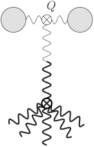
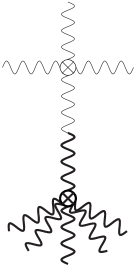
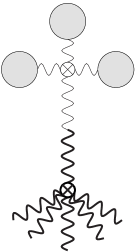
  Figure 1: The possible Feynman diagram configurations for Case 1. Fat lines refer to the new vertex $V_{i}$, while normal lines to the original theory.

• Case 2: the double attachment
  Let us assume that there are $\ell_{2}$ spots at which 2 legs arrive (see Figure 2), whereby evidently each time a loop is created. Also here, 4 configurations arise:

  1. $\ell_{2a}^{\prime}$ by using a 3-vertex with 1 external leg
     The following UV weight is found

     $$\mathcal{W}_{\ell_{2a}^{\prime}} \sim \left(\int\mathrm{d}^{3}Q\frac{1}{(Q^{2})^{2}}Q\right)^{\ell_{2a}^{\prime}}\sim 1\,.$$ (20)

     For the benefit of the reader, let us again explain the origin of the different components in the previous weight factor. There is a loop integral, the two propagators building the loop and an extra $Q$ corresponding to the 3-vertex (cfr Figure 2).

  2. $\ell_{2b}^{\prime}$ by using a 3-vertex with 0 external legs
     Using a slightly adapted argument, namely a pure “paste” one, we obtain in this case (see Figure 2)

     $$\mathcal{W}_{\ell_{2b}^{\prime}} \sim \left(\int(\mathrm{d}^{3}Q)^{2}\frac{1}{(Q^{2})^{3}}Q\right)^{\ell_{2b}^{\prime}}\sim Q^{\ell_{2b}^{\prime}}\,.$$ (21)

     Depicting the procedure for the reader: we attached 2 legs of the new vertex $V_{i}$ to a single external leg of the grey blob by means of 3-gluon vertex.

  3. $\ell_{2a}^{\prime\prime}$ by using a 4-vertex with 2 external legs
     Now one recovers (see Figure 2)

     $$\mathcal{W}_{\ell_{2a}^{\prime\prime}} \sim \left(\int\mathrm{d}^{3}Q\frac{1}{(Q^{2})^{2}}\right)^{\ell_{2a}^{\prime\prime}}\sim\frac{1}{Q^{\ell_{2a}^{\prime\prime}}}\,.$$ (22)

  4. $\ell_{2b}^{\prime\prime}$ by using a 4-vertex with 1 or 0 external legs
     For the fourth double attachment scenario (see Figure 2), we have

     $$\mathcal{W}_{\ell_{2b}^{\prime\prime}} \sim \left(\int(\mathrm{d}^{3}Q)^{2}\frac{1}{(Q^{2})^{3}}\right)^{\ell_{2b}^{\prime\prime}}\sim 1\,,$$ (23)

     which is obtained by the “cut & paste” logic.

  

  

  

  

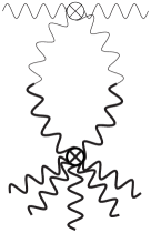
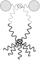
  Figure 2: The possible Feynman diagram configurations for Case 2.

• Case 3: the triple attachment
  Let us assume that there are $\ell_{3}$ spots at which 3 legs arrive. In this case, we observe 3 options:

  1. $\ell_{3}^{\prime}$ by using a 3-vertex
     This is the simplest case, as no external legs are available. We find

     $$\mathcal{W}_{\ell_{3}^{\prime}} \sim \left(\int(\mathrm{d}^{3}Q)^{2}\frac{1}{(Q^{2})^{3}}Q\right)^{\ell_{3}^{\prime}}\sim Q^{\ell_{3}^{\prime}}\,.$$ (24)

     There is a double loop integral, as it immediately follows from the diagram displayed in Figure 3

  2. $\ell_{3a}^{\prime\prime}$ by using a 4-vertex with 1 external leg
     From Figure 3, we find

     $$\mathcal{W}_{\ell_{3a}^{\prime\prime}} \sim \left(\int(\mathrm{d}^{3}Q)^{2}\frac{1}{(Q^{2})^{3}}\right)^{\ell_{3a}^{\prime\prime}}\sim 1\,.$$ (25)

  3. $\ell_{3b}^{\prime\prime}$ by using a 4-vertex with 0 external legs
     Once more employing the “cut & paste” argument leads us to

     $$\mathcal{W}_{\ell_{3b}^{\prime\prime}} \sim \left(\int(\mathrm{d}^{3}Q)^{3}\frac{1}{(Q^{2})^{4}}\right)^{\ell_{3b}^{\prime\prime}}\sim Q^{\ell_{3b}^{\prime\prime}}\,.$$ (26)

     The corresponding diagram is shown in Figure 3.

  

  

  

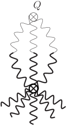
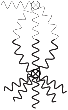
  Figure 3: The possible Feynman diagram configurations for Case 3.

• Case 4: the quadruple attachment
  Finally, we can assume that there are $\ell_{4}$ spots at which 4 legs arrive. Evidently, only one possibility pops up:

  $$\mathcal{W}_{\ell_{4}} \sim \left(\int(\mathrm{d}^{3}Q)^{3}\frac{1}{(Q^{2})^{4}}\right)^{\ell_{4}}\sim Q^{\ell_{4}}\,.$$ (27)

  This was obtained analogously as in Case 2.2.

  

  Figure 4: The possible Feynman diagram configuration for Case 4.

For later use, we mention that

$$\ell = \underbrace{\ell_{1a}^{\prime}+\ell_{1b}^{\prime}+\ell_{1a}^{\prime\prime}+\ell_{1b}^{\prime\prime}}_{=\ell_{1}}+2\underbrace{(\ell_{2a}^{\prime}+\ell_{2b}^{\prime}+\ell_{2a}^{\prime\prime}+\ell_{2b}^{\prime\prime})}_{=\ell_{2}}+3\underbrace{(\ell_{3}^{\prime}+\ell_{3a}^{\prime\prime}+\ell_{3b}^{\prime\prime})}_{=\ell_{3}}+4\ell_{4}\,,$$ (28)

which is readily checked.

We are now ready to combine all the obtained information into a single estimate for the UV weight,

$$\mathcal{W} \sim \frac{1}{Q^{3}}\mathcal{W}_{V}\mathcal{W}_{s}\mathcal{W}_{\ell_{1a}^{\prime}}\mathcal{W}_{\ell_{1b}^{\prime}}\mathcal{W}_{\ell_{1a}^{\prime\prime}}\mathcal{W}_{\ell_{1b}^{\prime\prime}}\mathcal{W}_{\ell_{2a}^{\prime}}\mathcal{W}_{\ell_{2b}^{\prime}}\mathcal{W}_{\ell_{2a}^{\prime\prime}}\mathcal{W}_{\ell_{2b}^{\prime\prime}}\mathcal{W}_{\ell_{3a}^{\prime}}\mathcal{W}_{\ell_{3a}^{\prime\prime}}\mathcal{W}_{\ell_{3b}^{\prime\prime}}\mathcal{W}_{\ell_{4}}\,.$$ (29)

We introduced a factor $\frac{1}{Q^{3}}$, which serves as a “correcting” weight factor related to local momentum conservation at the vertex $V_{i}$. During the derivation of the different weight factors, we have always assumed that the introduced loop integrals were independent, but momentum conservation at $V_{i}$ will at least kill one of these. Let us also mention here that the $e$ external momenta of $V_{i}$ will get related to the other external momenta of the final diagram by means of global momentum conservation.
Simplifying expression (29), we find for the total weight:

$$\mathcal{W}~{}\sim~{}\frac{1}{Q^{\kappa}}\;,$$

$$\text{with}\quad\kappa=(i-2)+3-s+\ell_{1a}^{\prime}+2\ell_{1a}^{\prime\prime}+\ell_{1b}^{\prime\prime}-\ell_{2b}^{\prime}+\ell_{2a}^{\prime\prime}-\ell_{3}^{\prime}-\ell_{3b}^{\prime\prime}-\ell_{4}\,.$$

The power $\kappa$ can be further simplified by means of (12) and (28), which leads to

$$\kappa=1+s+e+2\ell_{1a}^{\prime}+\ell_{1b}^{\prime}+3\ell_{1a}^{\prime\prime}+2\ell_{1b}^{\prime\prime}+2\ell_{2a}^{\prime}+\ell_{2b}^{\prime}+3\ell_{2a}^{\prime\prime}+2\ell_{2b}^{\prime\prime}+2\ell_{3}^{\prime\prime}+3\ell_{3a}^{\prime\prime}+2\ell_{3b}^{\prime\prime}+3\ell_{4}>0\,.$$ (31)

Recapitulating, the power of $\frac{1}{Q}$ is strictly positive, meaning that the UV weight $\mathcal{W}$, (2.2.3), of the new vertex is under control very well when $Q\sim\infty$.

So far, we have ignored the presence of quarks. The counting analysis will however remain valid even in that case. The only cases in which the 3-point quark-gluon vertex will appear and influence the power counting, correspond to the diagrams displayed in the figures 1 or 1. However, the situation corresponding to the case 1 is even further improved since the quark-gluon vertex does not contain an explicit momentum dependence. For the case of 1, we notice that the extra quark propagator will behave as $\frac{1}{Q}$ instead of $\frac{1}{Q^{2}}$, but since there is no $Q$ coming from the vertex itself, the eventual counting remains unaltered since “$\frac{1}{Q^{2}}Q=\frac{1}{Q}$”.

To close the inductive argument, we can of course repeat the previous argument when we allow a second, third, $\ldots$ new vertex of the type $V_{i}$ into where we are now: the theory plus one single vertex. The latter one has just been shown to behave well in the UV. We conclude that any number of new vertices added to the theory will only induce UV harmless additional (pieces of) diagrams.

Before closing this section, a few more words are to be devoted to the $i=2$ case. Setting $i=2$ (and thus $s=e=0$) in the UV estimate (2.2.3), we see that also the 2-legged insertion is UV safe when used to construct new diagrams starting from an originally renormalizable theory. In this case, this would be massless $3D$ YM, whose perturbation theory is unfortunately ill-defined. We can however circumvent this problem. In every “conventional” gauge, there exists a renormalizable (gauge variant) mass operator: the Landau [19], the linear covariant [20], the Curci-Ferrari [21], the maximal Abelian [21] and a class of nonlinear covariant gauges [22]. Strictly speaking, this was proven only in $4D$, with the exception of the Landau and Curci-Ferrari gauges which were also explicitly analyzed in $3D$ [10], but the algebraic renormalizability analysis of the mass operators does not really depend on the space time dimension, and all the relevant Ward identities will remain valid in $3D$. Continuing our reasoning, we choose a gauge to work in and add an IR regulating mass term to it. Starting from this theory, we can apply the foregoing arguments of this subsection also for the 2-legged insertion, and consequently conclude that $A^{2}_{\min}$ is power counting renormalizable in any of these gauges. Once this is established, we can drop again the temporarily introduced gauge variant mass term and immediately add the gauge invariant mass term $\propto A^{2}_{\min}$ to the action.

Summarizing, we have thus demonstrated that $A^{2}_{\min}$ should be power counting renormalizable in $3D$. The gauge invariant mass operator $A_{\min}^{2}$ should thus be consistent with the ultraviolet renormalizability. For practical calculations, it would still be technically challenging to calculate with $A^{2}_{\min}$ even in the Feynman gauge. However, since it is explicitly gauge invariant, we do not make any sacrifices choosing to work in the clearly preferable Landau gauge, in which case we have the relatively simple action (2) at our disposal. In this case, we also do not have to worry about the overabundance of $\frac{1}{\partial^{2}}$ in the expressions (3) or (4), which could cause IR troubles during the calculation of the Feynman integrals. Due to the gauge invariance and the subsequent choice of the Landau gauge where no potentially dangerous $\frac{1}{\partial^{2}}$ terms are present, it is obvious that these possible infrared divergences cannot influence physical quantities (they should cancel out if occurring in intermediate results). We shall come back to this issue at the end of section 3.

2.3 A more general class of powercounting renormalizable gauge invariant 2D operators and the preferred role of $A^{2}_{\min}$

As the attentive reader might have noticed, we can extract more interesting information from our proof than simply the UV powercounting renomalizability of $A^{2}_{\min}$. In fact, all the operators $\mathcal{O}_{i}$ are separately UV powercounting renomalizable. A fortiori, so is any (infinite) linear combination of those. However, there is more to the story in $3D$ than just UV powercounting renormalizability, we should also take the infrared safety into account. First of all, $\mathcal{O}_{2}$ should be present as this is the only one that will give rise to a mass in the gluon propagator, which can serve as a natural infrared cut-off. Secondly, we should also be aware of the potential infrared danger caused by the $\frac{1}{\partial^{2}}$’s in the interaction terms. It is exactly our point that by using a particular series of these operator, viz. $A^{2}_{\min}$, one can motivate that no infrared dangerous terms will occur when calculating gauge invariant quantities, as we have done at the end of the previous subsection.

3 Removal of the regulating mass parameter $m$

3.1 The inversion method

Albeit that we have regularized the $3D$ gauge theory in a gauge invariant fashion by the introduction of the mass $m$, it is still a mass introduced by hand. The next goal is to get rid of this arbitrary parameter.

We shall explain the inversion method with the example of the pole mass. Consider the one loop gauge boson polarization tensor $\pi_{\mu\nu}^{ab}$, which can be decomposed in the traditional way

$$\pi_{\mu\nu}^{ab}(q^{2})=\delta^{ab}\left(\delta_{\mu\nu}-\frac{q_{\mu}q_{\nu}}{q^{2}}\right)\pi(q^{2})+\delta^{ab}\frac{q_{\mu}q_{\nu}}{q^{2}}\omega(q^{2})\,.$$ (32)

It is then easily shown that the corresponding shift in the tree level mass will be given by

$$m^{2}\to m^{2}+\pi(q^{2})\,.$$ (33)

The pole mass (squared) $m_{p}^{2}$ is defined as that value of $(-q^{2})$ such that $q^{2}+m^{2}+\pi(q^{2})=0$. As we are working with a perturbative series, this can be solved in an iterative way, so that at lowest order

$$m_{p}^{2}=m^{2}+g^{2}\pi_{1}(-m^{2})\,,$$ (34)

where $\pi_{1}(q^{2})$ is the one loop contribution to the self energy.

Having found an expression for the pole mass $m_{p}$ in terms of the regulating mass $m$,

$$m_{p}^{2}=m^{2}\left(1+a_{1}\frac{g^{2}}{m}+a_{2}\frac{g^{4}}{m^{2}}+\ldots\right)\equiv m^{2}\mathcal{A}(m^{2})\,,$$ (35)

the question remains what we must do with it, since $m$ should in principle become zero again at the end of any calculation, to restore equivalence with the original starting massless YM action. One option is to simply set $m=0$ in (35). However, as outlined in [23], (certain) nonperturbative effects can be taken into account when the series (35) is inverted as follows,

$$m^{2}=m_{p}^{2}\left(1+b_{1}\frac{g^{2}}{m_{p}}+b_{2}\frac{g^{4}}{m_{p}^{2}}+\ldots\right)\equiv m_{p}^{2}\mathcal{B}(m_{p}^{2})\,.$$ (36)

Apparently, $m=0$ can now be realized in 2 ways: by setting $m_{p}=0$ corresponding to the perturbative (potentially ill-defined) solution, but also by solving the gap equation

$$\mathcal{B}(m_{p}^{2})=0\,,$$ (37)

which can give rise to a nontrivial solution $m_{p}^{2}\neq 0$, whereby that nevertheless $m=0$!

We used the example of the pole mass $m_{p}$ to explain the inversion philosophy, but also other quantities ${\cal Q}$ could be handled: the regulating mass $m$ is introduced to ensure a meaningful perturbative series for ${\cal Q}(m)$, and after inversion a meaningful (finite) result can be found for ${\cal Q}$ even for $m=0$, by solving the gap equation $m({\cal Q})=0$. Hence, it appears that the inversion method can be a very useful tool to obtain results in superrenormalizable quantum field theories, which are plagued by infrared instabilities.

3.2 Explicit calculations

We now turn to an explicit computation. We have calculated the gauge boson self energy at one loop by evaluating the contributing four Feynman diagrams in three dimensions where we also include massless quarks. The diagrams are generated by the Qgraf package, [24], and converted to Form input notation where Form is a symbolic manipulation language, [25]. The self energy is then reduced to a set of master one loop integrals which have previously been determined in [26]. Whilst these have been deduced in dimensional regularization in $d$ $=$ $3$ $-$ $2\epsilon$, the relevant one loop integrals are in fact finite in three dimensions. Hence we find that the transverse part of the self energy is

$$\pi(q^{2}) = -\frac{g^{2}}{8}T_{F}N_{f}\sqrt{q^{2}}+\frac{g^{2}N}{\pi}\left\{\frac{7}{32}m-\frac{1}{32}\frac{m^{3}}{q^{2}}+\frac{5}{32}\frac{q^{2}}{m}+\frac{5}{8}\sqrt{q^{2}}\mbox{ArcTan}\left(\frac{1}{2}\frac{\sqrt{q^{2}}}{m}\right)\right.$$ (38)

$$\left.-\frac{1}{2}\sqrt{q^{2}}\frac{m^{2}}{q^{2}}\mbox{ArcTan}\left(\frac{1}{2}\frac{\sqrt{q^{2}}}{m}\right)+\frac{1}{8}\sqrt{q^{2}}\frac{q^{2}}{m^{2}}\mbox{ArcTan}\left(\frac{1}{2}\frac{\sqrt{q^{2}}}{m}\right)\right.$$

$$\left.-\frac{1}{64}\sqrt{q^{2}}\frac{(q^{2})^{2}}{m^{4}}\mbox{ArcTan}\left(\frac{1}{2}\frac{\sqrt{q^{2}}}{m}\right)-\frac{5}{16}\sqrt{q^{2}}\mbox{ArcTan}\left(\frac{\sqrt{q^{2}}}{m}\right)\right.$$

$$\left.+\frac{1}{32}\sqrt{q^{2}}\frac{m^{4}}{(q^{2})^{2}}\mbox{ArcTan}\left(\frac{\sqrt{q^{2}}}{m}\right)-\frac{1}{8}\sqrt{q^{2}}\frac{m^{2}}{q^{2}}\mbox{ArcTan}\left(\frac{\sqrt{q^{2}}}{m}\right)\right.$$

$$\left.-\frac{1}{8}\sqrt{q^{2}}\frac{q^{2}}{m^{2}}\mbox{ArcTan}\left(\frac{\sqrt{q^{2}}}{m}\right)+\frac{1}{32}\sqrt{q^{2}}\frac{(q^{2})^{2}}{m^{4}}\mbox{ArcTan}\left(\frac{\sqrt{q^{2}}}{m}\right)\right\}$$

$$+g^{2}N\left\{\frac{1}{64}\sqrt{q^{2}}-\frac{1}{128}\sqrt{q^{2}}\frac{(q^{2})^{2}}{m^{4}}\right\}$$

for the transverse component, and

$$\omega(q^{2}) = \frac{g^{2}N}{\pi}\left\{-\frac{1}{16}m+\frac{1}{16}\frac{m^{3}}{q^{2}}-\frac{1}{16}\sqrt{q^{2}}\mbox{ArcTan}\left(\frac{\sqrt{q^{2}}}{m}\right)-\frac{1}{16}\sqrt{q^{2}}\frac{m^{4}}{(q^{2})^{2}}\mbox{ArcTan}\left(\frac{\sqrt{q^{2}}}{m}\right)\right.$$ (39)

$$\left.-\frac{1}{8}\sqrt{q^{2}}\frac{m^{2}}{q^{2}}\mbox{ArcTan}\left(\frac{\sqrt{q^{2}}}{m}\right)\right\}+g^{2}N\frac{\sqrt{q^{2}}}{32}$$

for the longitudinal component. The reader might be a little confused, as the computed 1-loop self energy $\pi_{\mu\nu}^{ab}$ is apparently not transverse. However, the Ward identity in the massive Landau case does not predict a transverse self energy. Details can be found in the Appendix.

3.3 Back to the pole mass

Let us return to the determination of the pole mass, at 1-loop given by

$$m_{p}^{2}=m^{2}+g^{2}\pi_{1}(-m^{2})\,.$$ (40)

A few complications arise. A first one is the appearance of $\mbox{ArcTan}(i)=i\infty$ in $\pi(-m^{2})$, but fortunately, these terms cancel amongst each other. Less fortunately, the presence of $\sqrt{q^{2}}$ results in a complex valued pole mass. We find

$$m_{p}^{2}=m^{2}-\frac{i}{8}T_{F}N_{f}g^{2}m+\frac{N}{\pi}\left(\frac{3}{32}-\frac{63}{128}\ln 3\right)g^{2}m+iN\frac{1}{128}g^{2}m+\ldots\,,$$ (41)

since $\mbox{ArcTan}\left(\frac{i}{2}\right)=\frac{i}{2}\ln 3$. Performing the inversion and solving the induced gap equation, we obtain

$$m_{p}=-\frac{i}{8}T_{F}N_{f}g^{2}+\frac{N}{\pi}\left(\frac{3}{32}-\frac{63}{128}\ln 3\right)g^{2}+iN\frac{1}{128}g^{2}+\ldots\,.$$ (42)

It is interesting that, using a different approach and different mass operators, the works [6, 7] also report a complex pole mass in some cases, depending on the employed (gauge invariant) mass operator.

We recall here that $3D$ gauge theories are also confining. This means that the gluon itself is not a physical particle, and as such, unitarity should not be expected at the level of the elementary gluon excitations. Therefore, we certainly do not claim that we have obtained massive gauge bosons with 3 physical polarizations, even if the eventual pole mass would have been real-valued. Notice that unitarity at the level of the gluons was also not mentioned in e.g. [6, 7]. The main point of these papers and the current work is to find a way to regulate the $3D$ gauge theory to allow for a consistent expansion. Once this is done, one could try to have a look at the physical excitations, which are supposed to be massive glueball states, a fact supported by the $3D$ lattice data [27]. For example, one could try to construct a bound state of gluons using standard techniques, or one could study gauge invariant correlators like $\langle F_{\mu\nu}^{2}(x)F_{\mu\nu}^{2}(y)\rangle$, since the operator $F_{\mu\nu}^{2}$ has the correct quantum numbers to create/annihilate a scalar glueball. This is however beyond the scope of this paper, but let us only underline that an explicit calculation of $\langle F_{\mu\nu}^{2}(x)F_{\mu\nu}^{2}(y)\rangle$ would also be plagued by infrared singularities in $3D$, unless some regulating mechanism is being provided.

3.4 Applying the inversion method to the gluon propagator

As a second example, we shall now determine an estimate for the gluon propagator. In our conventions, the gluon propagator reads

$$D(p)=\frac{1}{p^{2}+m^{2}+\pi(p^{2},m^{2})}\,,$$ (43)

which we have calculated explicitly to 1-loop order. For any value of the Euclidean momentum $p=p_{\ast}$, we can invert (43) to get $m^{2}=\mathcal{F}(D(p_{\ast}))$, and then solve $\mathcal{F}(D(p_{\ast}))=0$ in order to obtain a value for $D(p_{\ast})$. Since we have

$$\frac{1}{D(p)}=p^{2}+m^{2}+g^{2}\pi_{1}(p^{2},m^{2})$$ (44)

at lowest order, where the value of $\pi_{1}(p^{2},m^{2})$ can be extracted from (38), we can solve for $m^{2}$ in an iterative way as follows

$$m^{2}=\xi(p)-g^{2}\pi_{1}(p^{2},\xi)\,,$$ (45)

where we put $\xi(p)=\frac{1}{D(p)}-p^{2}$ for notational simplicity. Assuming that $\xi_{\ast}(p)$ obeys

$$\xi_{\ast}(p)-g^{2}\pi_{1}(p^{2},\xi_{\ast}(p))=0\,,$$ (46)

we arrive at the following 1-loop estimate for the $3D$ gluon propagator

$$D(p)=\frac{1}{p^{2}+\xi_{\ast}(p)}\,.$$ (47)

We plotted $D(p)$ as a function of $p$ in Figure 5.

Since we are still using a series expansion, one might wonder if we have any control over this expansion? We recall that the formal counting of the orders in the expansion is done by $g^{2}$, which unfortunately carries a dimension, hence $g^{2}$ is not really suitable as expansion parameter. However, taking a look at the inverted series (46), we notice that we can say that $\frac{g^{2}}{\sqrt{\xi_{*}}}$ will emerge as a natural dimensionless expansion parameter at each order. In addition, in a $D$-dimensional space time and in the absence of quarks ($N_{f}=0$), the coupling constant is always accompanied by an additional suppressing factor $\frac{N}{(4\pi)^{D/2}}$ due to the loop integrations. In Figure 6, we have therefore plotted the quantity $y(p)=\frac{g^{2}N}{(4\pi)^{3/2}\sqrt{\xi_{*}(p)}}$ in function of the momentum $p$. We recognize this is a rude way of estimating the acceptability of a perturbative approach, but at least we can be satisfied that $y$ is sufficiently small if we do not come too close to zero momentum.

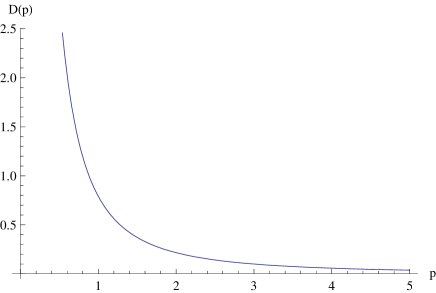
Figure 5: The gluon propagator $D(p)$, in units $g^{2}=1$, for $N=3$.

Figure 6: The expansion parameter $y$, for $N=3$.

3.5 A few extra words on $A^{2}_{\min}$ beyond the Landau gauge

We recall that $A^{2}$ is not gauge invariant, but in the Landau gauge it equals $A^{2}_{\min}$, and we motivated that the latter gauge invariant quantity is power counting renormalizable in $3D$, assuring that we in principle considered a gauge invariant regularization. We draw attention to the fact that the ghost in the Landau gauge is still massless, and might introduce additional infrared instabilities. In order to overcome these, one might consider using the Curci-Ferrari gauge, a generalization of the Landau gauge, in which case the ghosts also attain a mass [10, 11]. At the end of such a calculation, the limit to the Landau gauge can be considered. However, since the ghost mass is explicitly gauge parameter dependent, it will not enter gauge invariant quantities, and as such, the Landau gauge could be immediately used to calculate gauge invariant quantities without risking extra infrared divergences.

The question remains what to do if we would like to calculate e.g. the gluon propagator $D(p)$ in the linear covariant gauges with $A^{2}_{\min}$? Infrared singularities coming from the $\frac{1}{\partial^{2}}$’s in (5) can be avoided by using

$$S_{m} = m^{2}\mbox{Tr}\int\mathrm{d}^{3}x\left(F_{\mu\nu}\frac{1}{D^{2}+\rho^{2}}F_{\mu\nu}+2ig\frac{1}{D^{2}+\rho^{2}}F_{\lambda\mu}\left[\frac{1}{D^{2}+\rho^{2}}D_{\kappa}F_{\kappa\lambda},\frac{1}{D^{2}+\rho^{2}}D_{\nu}F_{\nu\mu}\right]\right.$$ (48)

$$-2ig\left.\frac{1}{D^{2}+\rho^{2}}F_{\lambda\mu}\left[\frac{1}{D^{2}+\rho^{2}}D_{\kappa}F_{\kappa\nu},\frac{1}{D^{2}+\rho^{2}}D_{\nu}F_{\lambda\mu}\right]\right)+\mathcal{O}(F^{4})$$

instead of (5). We introduced an extra mass parameter $\rho^{2}$, but neither the gauge invariance nor good UV behaviour are compromised by this. The potentially dangerous $\frac{1}{\partial^{2}}$ will get replaced by the IR safe $\frac{1}{\partial^{2}+\rho^{2}}$. As such, we will get a well defined $D(p,m^{2},\rho^{2})$. Once this is done, one can check whether the limit $\rho^{2}\to 0$ exists or not. In the Landau gauge, this should be the case as already explained before, in which case we are back to $A^{2}_{\min}$. If not, one can perform a first inversion with respect to $\rho^{2}$ to find a sensible $D(p,m^{2})$, starting from which a second inversion can be done to ensure $m^{2}=0$.

4 Discussion

The purpose of this paper was to illustrate that inclusion of the operator $A^{2}$ in combination with the inversion method allows for a consistent (i.e. infrared protected) perturbative expansion of basically any quantity. However, there are other major sources of effects beyond (regularized) perturbation theory. For example, we can mention the existence of Gribov (gauge) copies in the Landau gauge. Trying to restrict the integration measure in order to take these copies into account, can have a profound influence on the gluon propagator, analogously as in $4D$ [28]. The restriction introduces another mass scale $\gamma$ in the theory [29], and we can expect that $\gamma\propto g^{2}$ in $3D$. A standard Gribov-like propagator looks like $\frac{p^{2}}{p^{4}+\gamma^{4}}$, clearly having 2 complex poles at $p^{2}=\pm i\gamma^{2}$. The Gribov restriction is important as a theoretical tool to find a violation of positivity in the gluon propagator, indicative of confinement [29]. In this light, dynamical gluon mass scales, complex or real, should not be directly related to massive “physical” gluons, as these are confined and hence unphysical. Therefore, a complex pole mass as found here or in other works [6, 7] is not necessarily a catastrophe. We recall that $3D$ gauge theories, although that the classical/perturbative interaction potential is already mildly (viz. logarithmically) confining, also display “true” confinement trough a linear potential, see e.g. [27]. The origin of this piece of the potential is not evident.

When we compare our propagator displayed in Figure 5 with the lattice result of [30], then it is immediately clear that the big difference is located in the deep infrared: the lattice results indicate a finite gluon propagator near zero momentum. But at larger momenta, the inversion mechanism described in this paper which regulates the theory can give acceptable results.

To conclude, it would be recommendable to pursue e.g. an analytical study in $3D$ based on [31] taking into account the existence of Gribov copies, and find out whether a more qualititative agreement with the available lattice data can be found also in $3D$ [29, 32]. At the same time, it can be investigated whether the Gribov scale $\gamma$ would serve as a natural IR regulator.

Appendix A The Ward identity for the gluon self energy

We start from the complete classical action

$$\Sigma = S_{\mathrm{YM}}+S_{\mathrm{Landau}}+S_{\mathrm{ext}}+s\int\mathrm{d}^{3}\!x\,\biggl{(}\frac{1}{2}\tau A^{a}_{\mu}A^{a}_{\mu}\biggr{)}$$ (49)

$$= \int\mathrm{d}^{3}\!x\,\biggl{(}\frac{1}{4}F^{a}_{\mu\nu}F^{a}_{\mu\nu}+b^{a}\partial_{\mu}A^{a}_{\mu}+\overline{c}^{a}\partial_{\mu}D_{\mu}^{ab}c^{b}+\frac{1}{2}JA^{a}_{\mu}A^{a}_{\mu}+\tau A^{a}_{\mu}\partial_{\mu}c^{a}-\Omega^{a}_{\mu}D_{\mu}^{ab}c^{b}+\frac{g}{2}f^{abc}L^{a}c^{b}c^{c}\biggr{)}\;,$$

supplemented with the necessary extra (external) source terms, e.g. $J$ which is used to couple the operator $A^{2}$ to the theory. Moreover, $s$ denotes the usual BRST symmetry generator,

$$sA_{\mu}^{a}=-\left(D_{\mu}c\right)^{a}\,,\qquad sc^{a}=\frac{1}{2}gf^{abc}c^{b}c^{c}\,,\qquad s\overline{c}^{a}=b^{a}\,,\qquad sb^{a}=0\,,$$ (50)

extended to the sources by means of

$$s\tau=J\,,\qquad sJ=0\,,\qquad s\Omega^{a}_{\mu}=0\,,\qquad sL^{a}=0.$$ (51)

The corresponding Slavnov-Taylor identity reads

$$\mathcal{S}(\Sigma)=\int\mathrm{d}^{3}\!x\,\biggl{(}\frac{\delta\Sigma}{\delta\Omega_{\mu}^{a}}\frac{\delta\Sigma}{\delta A_{\mu}^{a}}+\frac{\delta\Sigma}{\delta L^{a}}\frac{\delta\Sigma}{\delta c^{a}}+b^{a}\frac{\delta\Sigma}{\delta\overline{c}^{a}}+J\frac{\delta\Sigma}{\delta\tau}\biggr{)}=0\;.$$ (52)

The Ward identity for the vacuum polarization can be derived from this Slavnov-Taylor identity, suitably extended to the quantum level. At the one loop level, one has

$$\Gamma=\Sigma+\hbar\Gamma^{1}\;,$$ (53)

so that the 1-loop Slavnov-Taylor identity becomes

$$\int\mathrm{d}^{3}x\left(\frac{\delta\Gamma^{1}}{\delta\Omega_{\mu}^{a}}\frac{\delta\Sigma}{\delta A_{\mu}^{a}}+\frac{\delta\Sigma}{\delta\Omega_{\mu}^{a}}\frac{\delta\Gamma^{1}}{\delta A_{\mu}^{a}}+\frac{\delta\Gamma^{1}}{\delta L^{a}}\frac{\delta\Sigma}{\delta c^{a}}+\frac{\delta\Sigma}{\delta L^{a}}\frac{\delta\Gamma^{1}}{\delta c^{a}}+b^{a}\frac{\delta\Gamma^{1}}{\delta\overline{c}^{a}}+J\frac{\delta\Gamma^{1}}{\delta\tau}\right)=0\,.$$

(54)

Using

$$\frac{\delta\Gamma^{1}}{\delta\Omega_{\mu}^{a}} = \left[-\left(D_{\mu}^{ab}c^{b}\right)\cdot\Gamma\right]^{1}\;,\quad\frac{\delta\Gamma^{1}}{\delta L^{a}}=\left[\left(\frac{g}{2}f^{abc}c^{b}c^{c}\;\right)\cdot\Gamma\right]^{1}\;,\quad\frac{\delta\Gamma^{1}}{\delta\tau}=\left[\left(A_{\mu}^{a}\partial_{\mu}c^{a}\right)\;\cdot\Gamma\right]^{1}\,,$$ (55)

we derive

$$\int\mathrm{d}^{3}x\left(\left[-\left(D_{\mu}^{ab}c^{b}\right)\cdot\Gamma\right]^{1}\frac{\delta\Sigma}{\delta A_{\mu}^{a}}-\left(D_{\mu}^{ab}c^{b}\right)\frac{\delta\Gamma^{1}}{\delta A_{\mu}^{a}}+\left[\left(\frac{g}{2}f^{abc}c^{b}c^{c}\;\right)\cdot\Gamma\right]^{1}\frac{\delta\Sigma}{\delta c^{a}}\right.$$ (56)

$$+ \left.\left(\frac{g}{2}f^{abc}c^{b}c^{c}\;\right)\frac{\delta\Gamma^{1}}{\delta c^{a}}+J\left[\left(A_{\mu}^{a}\partial_{\mu}c^{a}\right)\;\cdot\Gamma\right]^{1}+b^{a}\frac{\delta\Gamma^{1}}{\delta\overline{c}^{a}}\right)=0\,.$$

Applying the test operator $\frac{\delta^{2}}{\delta c^{a}(x)\delta A_{\nu}^{b}(y)}$ and setting all fields and sources equal to zero at the end of the operation, except for $J=m^{2}$, one obtains the Ward identity for the vacuum polarization $\pi_{\mu\nu}^{ab}$

$$\partial_{\mu}\pi_{\mu\nu}^{ab}(x,y)\equiv\partial_{\mu}^{x}\frac{\delta^{2}\Gamma^{1}}{\delta A_{\mu}^{a}(x)\delta A_{v}^{b}(y)}=-m^{2}\left(\frac{\delta^{2}\left[\displaystyle\int\mathrm{d}^{3}z\left(A_{\mu}^{a}\partial_{\mu}c^{a}\right)_{z}\;\cdot\Gamma\right]^{1}}{\delta c^{a}(x)\delta A_{\nu}^{b}(y)}\right)+m^{2}\left(\frac{\delta\left[\displaystyle\left(D_{\nu}^{bd}c^{d}\right)_{y}\;\cdot\Gamma\right]^{1}}{\delta c^{a}(x)}\right)\,.$$ (57)

The first term is trivial, by using partial integration and the fact that we are considering the Landau gauge $\partial A=0$. Hence, the vacuum polarization in the massive Landau case is not transverse, but rather subject to the following Ward identity at one loop

$$\partial_{\mu}\pi_{\mu\nu}^{ab}(x,y)=m^{2}\left(\frac{\delta\left[\displaystyle\left(D_{\nu}^{bd}c^{d}\right)_{y}\;\cdot\Gamma\right]^{1}}{\delta c^{a}(x)}\right)\,.$$ (58)

References

- [1] T. Appelquist and R. D. Pisarski, Phys. Rev. D 23 (1981) 2305.
- [2] M. Franz and Z. Tešanović, Phys. Rev. Lett. 87 (2001) 257003.
- [3] R. Jackiw and S. Templeton, Phys. Rev. D 23 (1981) 2291.
- [4] W. Buchmuller and O. Philipsen, Nucl. Phys. B 443 (1995) 47.
- [5] G. Alexanian and V. P. Nair, Phys. Lett. B 352 (1995) 435.
- [6] R. Jackiw and S. Y. Pi, Phys. Lett. B 368 (1996) 131.
- [7] R. Jackiw and S. Y. Pi, Phys. Lett. B 403 (1997) 297.
- [8] D. Karabali and V. P. Nair, Int. J. Mod. Phys. A 12 (1997) 1161.
- [9] O. Philipsen in TFT98: Proceedings of the 5th International Workshop on Thermal Field Theories and Their Applications, edited by U. W. Heinz.
- [10] D. Dudal, J. A. Gracey, V. E. R. Lemes, R. F. Sobreiro, S. P. Sorella and H. Verschelde, Annals Phys. 317 (2005) 203.
- [11] D. Dudal, J. A. Gracey, R. F. Sobreiro, S. P. Sorella and H. Verschelde, Phys. Rev. D 75 (2007) 061701.
- [12] M. Lavelle and D. McMullan, Phys. Rept. 279 (1997) 1.
- [13] J. A. Gracey, Phys. Lett. B 651 (2007) 253.
- [14] D. Zwanziger, Nucl. Phys. B 345 (1990) 461.
- [15] M. A. L. Capri, D. Dudal, J. A. Gracey, V. E. R. Lemes, R. F. Sobreiro, S. P. Sorella and H. Verschelde, Phys. Rev. D 72 (2005) 105016.
- [16] M. A. L. Capri, D. Dudal, J. A. Gracey, V. E. R. Lemes, R. F. Sobreiro, S. P. Sorella and H. Verschelde, Phys. Rev. D 74 (2006) 045008.
- [17] H. Verschelde, K. Knecht, K. Van Acoleyen and M. Vanderkelen, Phys. Lett. B 516 (2001) 307.
- [18] J. A. Gracey, Phys. Lett. B 552 (2003) 101.
- [19] D. Dudal, H. Verschelde and S. P. Sorella, Phys. Lett. B 555 (2003) 126.
- [20] D. Dudal, H. Verschelde, V. E. R. Lemes, M. S. Sarandy, R. F. Sobreiro, S. P. Sorella and J. A. Gracey, Phys. Lett. B 574 (2003) 325.
- [21] D. Dudal, V. E. R. Lemes, M. S. Sarandy, R. Sobreiro, S. P. Sorella, M. Picariello, J .A. Gracey and H. Verschelde, Phys. Lett. B 569 (2003) 57.
- [22] V. E. R. Lemes, R. F. Sobreiro and S. P. Sorella, J. Phys. A 40 (2007) 4025.
- [23] R. Fukuda, Phys. Rev. Lett. 61 (1988) 1549.
- [24] P. Nogueira, J. Comput. Phys. 105 (1993) 279.
- [25] J. A. M. Vermaseren, math-ph/0010025.
- [26] A. K. Rajantie, Nucl. Phys. B 480 (1996) 729 [Erratum-ibid. B 513 (1998)].
- [27] M. J. Teper, Phys. Rev. D 59 (1999) 014512.
- [28] V. N. Gribov, Nucl. Phys. B 139 (1978) 1.
- [29] A. Cucchieri, T. Mendes and A. R. Taurines, Phys. Rev. D 71 (2005) 051902.
- [30] A. Cucchieri, T. Mendes and A. R. Taurines, Phys. Rev. D 67 (2003) 091502.
- [31] D. Dudal, S. P. Sorella, N. Vandersickel and H. Verschelde, Phys. Rev. D 77 (2008) 071501.
- [32] A. Cucchieri and T. Mendes, PoS LAT2007 (2007) 297.