1 Preliminaries
The equations of motion of the Kowalevski top in two constant fields, expressed in the
reference system O 𝐞 1 𝐞 2 𝐞 3 𝑂 subscript 𝐞 1 subscript 𝐞 2 subscript 𝐞 3 O{\bf e}_{1}{\bf e}_{2}{\bf e}_{3} O 𝑂 O
2 ω ˙ 1 = ω 2 ω 3 + β 3 , 2 ω ˙ 2 = − ω 1 ω 3 − α 3 , ω ˙ 3 = α 2 − β 1 , α ˙ 1 = α 2 ω 3 − α 3 ω 2 , β ˙ 1 = β 2 ω 3 − β 3 ω 2 , α ˙ 2 = α 3 ω 1 − α 1 ω 3 , β ˙ 2 = β 3 ω 1 − β 1 ω 3 , α ˙ 3 = α 1 ω 2 − α 2 ω 1 , β ˙ 3 = β 1 ω 2 − β 2 ω 1 formulae-sequence 2 subscript ˙ 𝜔 1 subscript 𝜔 2 subscript 𝜔 3 subscript 𝛽 3 formulae-sequence 2 subscript ˙ 𝜔 2 subscript 𝜔 1 subscript 𝜔 3 subscript 𝛼 3 subscript ˙ 𝜔 3 subscript 𝛼 2 subscript 𝛽 1 formulae-sequence subscript ˙ 𝛼 1 subscript 𝛼 2 subscript 𝜔 3 subscript 𝛼 3 subscript 𝜔 2 subscript ˙ 𝛽 1 subscript 𝛽 2 subscript 𝜔 3 subscript 𝛽 3 subscript 𝜔 2 formulae-sequence subscript ˙ 𝛼 2 subscript 𝛼 3 subscript 𝜔 1 subscript 𝛼 1 subscript 𝜔 3 subscript ˙ 𝛽 2 subscript 𝛽 3 subscript 𝜔 1 subscript 𝛽 1 subscript 𝜔 3 formulae-sequence subscript ˙ 𝛼 3 subscript 𝛼 1 subscript 𝜔 2 subscript 𝛼 2 subscript 𝜔 1 subscript ˙ 𝛽 3 subscript 𝛽 1 subscript 𝜔 2 subscript 𝛽 2 subscript 𝜔 1 \begin{array}[]{c}2\dot{\omega}_{1}=\omega_{2}\omega_{3}+\beta_{3},\;\quad 2\dot{\omega}_{2}=-\omega_{1}\omega_{3}-\alpha_{3},\;\quad\dot{\omega}_{3}=\alpha_{2}-\beta_{1},\\
\dot{\alpha}_{1}=\alpha_{2}\omega_{3}-\alpha_{3}\omega_{2},\;\quad\dot{\beta}_{1}=\beta_{2}\omega_{3}-\beta_{3}\omega_{2},\\
\dot{\alpha}_{2}=\alpha_{3}\omega_{1}-\alpha_{1}\omega_{3},\;\quad\dot{\beta}_{2}=\beta_{3}\omega_{1}-\beta_{1}\omega_{3},\\
\dot{\alpha}_{3}=\alpha_{1}\omega_{2}-\alpha_{2}\omega_{1},\;\quad\dot{\beta}_{3}=\beta_{1}\omega_{2}-\beta_{2}\omega_{1}\end{array} (1.1)
can without loss of generality be restricted to the phase space P 6 ⊂ 𝐑 9 ( 𝝎 , 𝜶 , 𝜷 ) superscript 𝑃 6 superscript 𝐑 9 𝝎 𝜶 𝜷 P^{6}\subset{\bf{R}}^{9}({\boldsymbol{\omega}},{\boldsymbol{\alpha}},{\boldsymbol{\beta}})
α 1 2 + α 2 2 + α 3 2 = a 2 , β 1 2 + β 2 2 + β 3 2 = b 2 , α 1 β 1 + α 2 β 2 + α 3 β 3 = 0 formulae-sequence superscript subscript 𝛼 1 2 superscript subscript 𝛼 2 2 superscript subscript 𝛼 3 2 superscript 𝑎 2 formulae-sequence superscript subscript 𝛽 1 2 superscript subscript 𝛽 2 2 superscript subscript 𝛽 3 2 superscript 𝑏 2 subscript 𝛼 1 subscript 𝛽 1 subscript 𝛼 2 subscript 𝛽 2 subscript 𝛼 3 subscript 𝛽 3 0 \alpha_{1}^{2}+\alpha_{2}^{2}+\alpha_{3}^{2}=a^{2},\quad\beta_{1}^{2}+\beta_{2}^{2}+\beta_{3}^{2}=b^{2},\quad\alpha_{1}\beta_{1}+\alpha_{2}\beta_{2}+\alpha_{3}\beta_{3}=0 (1.2)
(see [1 ] for details). This system is completely integrable
due to the existence of three integrals in involution
[2 , 3 ]
H = ω 1 2 + ω 2 2 + 1 2 ω 3 2 − ( α 1 + β 2 ) , K = ( ω 1 2 − ω 2 2 + α 1 − β 2 ) 2 + ( 2 ω 1 ω 2 + α 2 + β 1 ) 2 , G = 1 4 ( M α 2 + M β 2 ) + 1 2 ω 3 M γ − b 2 α 1 − a 2 β 2 , 𝐻 superscript subscript 𝜔 1 2 superscript subscript 𝜔 2 2 1 2 superscript subscript 𝜔 3 2 subscript 𝛼 1 subscript 𝛽 2 𝐾 superscript superscript subscript 𝜔 1 2 superscript subscript 𝜔 2 2 subscript 𝛼 1 subscript 𝛽 2 2 superscript 2 subscript 𝜔 1 subscript 𝜔 2 subscript 𝛼 2 subscript 𝛽 1 2 𝐺 1 4 superscript subscript 𝑀 𝛼 2 superscript subscript 𝑀 𝛽 2 1 2 subscript 𝜔 3 subscript 𝑀 𝛾 superscript 𝑏 2 subscript 𝛼 1 superscript 𝑎 2 subscript 𝛽 2 \begin{array}[]{l}\displaystyle{H=\omega_{1}^{2}+\omega_{2}^{2}+\frac{1}{2}\omega_{3}^{2}-(\alpha_{1}+\beta_{2}),}\\[8.53581pt]
K=(\omega_{1}^{2}-\omega_{2}^{2}+\alpha_{1}-\beta_{2})^{2}+(2\omega_{1}\omega_{2}+\alpha_{2}+\beta_{1})^{2},\\[8.53581pt]
\displaystyle{G=\frac{1}{4}(M_{\alpha}^{2}+M_{\beta}^{2})+\frac{1}{2}\omega_{3}M_{\gamma}-b^{2}\alpha_{1}-a^{2}\beta_{2},}\end{array} (1.3)
where
M α = 2 ω 1 α 1 + 2 ω 2 α 2 + ω 3 α 3 , M β = 2 ω 1 β 1 + 2 ω 2 β 2 + ω 3 β 3 , M γ = 2 ω 1 ( α 2 β 3 − α 3 β 2 ) + 2 ω 2 ( α 3 β 1 − α 1 β 3 ) + ω 3 ( α 1 β 2 − α 2 β 1 ) . subscript 𝑀 𝛼 2 subscript 𝜔 1 subscript 𝛼 1 2 subscript 𝜔 2 subscript 𝛼 2 subscript 𝜔 3 subscript 𝛼 3 subscript 𝑀 𝛽 2 subscript 𝜔 1 subscript 𝛽 1 2 subscript 𝜔 2 subscript 𝛽 2 subscript 𝜔 3 subscript 𝛽 3 subscript 𝑀 𝛾 2 subscript 𝜔 1 subscript 𝛼 2 subscript 𝛽 3 subscript 𝛼 3 subscript 𝛽 2 2 subscript 𝜔 2 subscript 𝛼 3 subscript 𝛽 1 subscript 𝛼 1 subscript 𝛽 3 subscript 𝜔 3 subscript 𝛼 1 subscript 𝛽 2 subscript 𝛼 2 subscript 𝛽 1 \begin{array}[]{l}M_{\alpha}=2\omega_{1}\alpha_{1}+2\omega_{2}\alpha_{2}+\omega_{3}\alpha_{3},\\
M_{\beta}=2\omega_{1}\beta_{1}+2\omega_{2}\beta_{2}+\omega_{3}\beta_{3},\\
M_{\gamma}=2\omega_{1}(\alpha_{2}\beta_{3}-\alpha_{3}\beta_{2})+2\omega_{2}(\alpha_{3}\beta_{1}-\alpha_{1}\beta_{3})+\omega_{3}(\alpha_{1}\beta_{2}-\alpha_{2}\beta_{1}).\end{array} (1.4)
For the general case
the explicit integration has not been found yet. It is natural to
study first the invariant submanifolds in P 6 superscript 𝑃 6 P^{6} [4 , 1 ] that there exist only three submanifolds
𝔐 , 𝔑 , 𝔒 𝔐 𝔑 𝔒
\mathfrak{M},\mathfrak{N},\mathfrak{O} 𝔐 ∪ 𝔑 ∪ 𝔒 𝔐 𝔑 𝔒 \mathfrak{M}\cup\mathfrak{N}\cup\mathfrak{O}
H × K × G : P 6 → 𝐑 3 . : 𝐻 𝐾 𝐺 → superscript 𝑃 6 superscript 𝐑 3 H\times K\times G:P^{6}\to{\bf{R}}^{3}. (1.6)
If b = 0 𝑏 0 b=0 [5 ] ), then the
critical set of the map (1.6 [6 ] . The set
𝔐 𝔐 \mathfrak{M} [2 ] as the zero level of the
integral K 𝐾 K 𝔐 𝔐 \mathfrak{M} [7 ] . The dynamical system on 𝔑 𝔑 \mathfrak{N} [8 ] . The present work considers the restriction of
the system (1.1 𝔒 𝔒 \mathfrak{O}
Introduce the complex phase variables [9 ] (i 2 = − 1 superscript 𝑖 2 1 i^{2}=-1
x 1 = ( α 1 − β 2 ) + i ( α 2 + β 1 ) , x 2 = ( α 1 − β 2 ) − i ( α 2 + β 1 ) , y 1 = ( α 1 + β 2 ) + i ( α 2 − β 1 ) , y 2 = ( α 1 + β 2 ) − i ( α 2 − β 1 ) , z 1 = α 3 + i β 3 , z 2 = α 3 − i β 3 , w 1 = ω 1 + i ω 2 , w 2 = ω 1 − i ω 2 , w 3 = ω 3 . formulae-sequence subscript 𝑥 1 subscript 𝛼 1 subscript 𝛽 2 𝑖 subscript 𝛼 2 subscript 𝛽 1 subscript 𝑥 2 subscript 𝛼 1 subscript 𝛽 2 𝑖 subscript 𝛼 2 subscript 𝛽 1 formulae-sequence subscript 𝑦 1 subscript 𝛼 1 subscript 𝛽 2 𝑖 subscript 𝛼 2 subscript 𝛽 1 subscript 𝑦 2 subscript 𝛼 1 subscript 𝛽 2 𝑖 subscript 𝛼 2 subscript 𝛽 1 formulae-sequence subscript 𝑧 1 subscript 𝛼 3 𝑖 subscript 𝛽 3 subscript 𝑧 2 subscript 𝛼 3 𝑖 subscript 𝛽 3 formulae-sequence subscript 𝑤 1 subscript 𝜔 1 𝑖 subscript 𝜔 2 formulae-sequence subscript 𝑤 2 subscript 𝜔 1 𝑖 subscript 𝜔 2 subscript 𝑤 3 subscript 𝜔 3 \begin{array}[]{l}x_{1}=(\alpha_{1}-\beta_{2})+i(\alpha_{2}+\beta_{1}),\quad x_{2}=(\alpha_{1}-\beta_{2})-i(\alpha_{2}+\beta_{1}),\\
y_{1}=(\alpha_{1}+\beta_{2})+i(\alpha_{2}-\beta_{1}),\quad y_{2}=(\alpha_{1}+\beta_{2})-i(\alpha_{2}-\beta_{1}),\\
z_{1}=\alpha_{3}+i\beta_{3},\quad z_{2}=\alpha_{3}-i\beta_{3},\\
w_{1}=\omega_{1}+i\omega_{2},\quad w_{2}=\omega_{1}-i\omega_{2},\quad w_{3}=\omega_{3}.\end{array} (1.7)
The system (1.1
x 1 ′ = − x 1 w 3 + z 1 w 1 , x 2 ′ = x 2 w 3 − z 2 w 2 , y 1 ′ = − y 1 w 3 + z 2 w 1 , y 2 ′ = y 2 w 3 − z 1 w 2 , 2 z 1 ′ = x 1 w 2 − y 2 w 1 , 2 z 2 ′ = − x 2 w 1 + y 1 w 2 , 2 w 1 ′ = − ( w 1 w 3 + z 1 ) , 2 w 2 ′ = w 2 w 3 + z 2 , 2 w 3 ′ = y 2 − y 1 . subscript superscript 𝑥 ′ 1 subscript 𝑥 1 subscript 𝑤 3 subscript 𝑧 1 subscript 𝑤 1 subscript superscript 𝑥 ′ 2 subscript 𝑥 2 subscript 𝑤 3 subscript 𝑧 2 subscript 𝑤 2 subscript superscript 𝑦 ′ 1 subscript 𝑦 1 subscript 𝑤 3 subscript 𝑧 2 subscript 𝑤 1 subscript superscript 𝑦 ′ 2 subscript 𝑦 2 subscript 𝑤 3 subscript 𝑧 1 subscript 𝑤 2 2 subscript superscript 𝑧 ′ 1 subscript 𝑥 1 subscript 𝑤 2 subscript 𝑦 2 subscript 𝑤 1 2 subscript superscript 𝑧 ′ 2 subscript 𝑥 2 subscript 𝑤 1 subscript 𝑦 1 subscript 𝑤 2 formulae-sequence 2 subscript superscript 𝑤 ′ 1 subscript 𝑤 1 subscript 𝑤 3 subscript 𝑧 1 formulae-sequence 2 subscript superscript 𝑤 ′ 2 subscript 𝑤 2 subscript 𝑤 3 subscript 𝑧 2 2 subscript superscript 𝑤 ′ 3 subscript 𝑦 2 subscript 𝑦 1 \begin{array}[]{c}\begin{array}[]{ll}{x^{\prime}_{1}=-x_{1}w_{3}+z_{1}w_{1},}&{x^{\prime}_{2}=x_{2}w_{3}-z_{2}w_{2},}\cr{y^{\prime}_{1}=-y_{1}w_{3}+z_{2}w_{1},}&{y^{\prime}_{2}=y_{2}w_{3}-z_{1}w_{2},}\cr{2z^{\prime}_{1}=x_{1}w_{2}-y_{2}w_{1},}&{2z^{\prime}_{2}=-x_{2}w_{1}+y_{1}w_{2},}\end{array}\\
2w^{\prime}_{1}=-(w_{1}w_{3}+z_{1}),\quad 2w^{\prime}_{2}=w_{2}w_{3}+z_{2},\quad 2w^{\prime}_{3}=y_{2}-y_{1}.\end{array} (1.8)
Here the prime stands for d / d ( i t ) 𝑑 𝑑 𝑖 𝑡 d/d(it)
The set 𝔒 𝔒 \mathfrak{O} [1 ] , includes as a proper subset the following points
w 1 = w 2 = 0 , z 1 = z 2 = 0 . formulae-sequence subscript 𝑤 1 subscript 𝑤 2 0 subscript 𝑧 1 subscript 𝑧 2 0 w_{1}=w_{2}=0,\quad z_{1}=z_{2}=0. (1.9)
The invariant relations (1.9 [4 ]
𝜶 = a ( 𝐞 1 cos θ − 𝐞 2 sin θ ) , 𝜷 = ± b ( 𝐞 1 sin θ + 𝐞 2 cos θ ) , 𝜶 × 𝜷 ≡ ± a b 𝐞 3 , 𝝎 = d θ d t 𝐞 3 , d 2 θ d t 2 = − ( a ± b ) sin θ . formulae-sequence 𝜶 𝑎 subscript 𝐞 1 𝜃 subscript 𝐞 2 𝜃 𝜷 plus-or-minus 𝑏 subscript 𝐞 1 𝜃 subscript 𝐞 2 𝜃 formulae-sequence 𝜶 𝜷 plus-or-minus 𝑎 𝑏 subscript 𝐞 3 formulae-sequence 𝝎 𝑑 𝜃 𝑑 𝑡 subscript 𝐞 3 superscript 𝑑 2 𝜃 𝑑 superscript 𝑡 2 plus-or-minus 𝑎 𝑏 𝜃 \begin{array}[]{l}{\boldsymbol{\alpha}}=a({\bf{e}}_{1}\cos\theta-{\bf{e}}_{2}\sin\theta),\quad{\boldsymbol{\beta}}=\pm\,b({\bf{e}}_{1}\sin\theta+{\bf{e}}_{2}\cos\theta),\\[5.69054pt]
{\boldsymbol{\alpha}}\times{\boldsymbol{\beta}}\equiv\pm\,ab\,{\bf{e}}_{3},\quad\displaystyle{{\boldsymbol{\omega}}=\frac{d\theta}{dt}\,{\bf{e}}_{3},\quad\frac{d^{2}\theta}{dt^{2}}=-(a\pm b)\sin\theta.}\end{array} (1.10)
The corresponding values of the integrals (1.3
g = ± a b h , k = ( a ∓ b ) 2 , h ⩾ − ( a ± b ) . formulae-sequence 𝑔 plus-or-minus 𝑎 𝑏 ℎ formulae-sequence 𝑘 superscript minus-or-plus 𝑎 𝑏 2 ℎ plus-or-minus 𝑎 𝑏 g=\pm\,ab\,h,\quad k=(a\mp b)^{2},\quad h\geqslant-(a\pm b). (1.11)
In the sequel we use functions and expressions having singularities
at the points (1.9 1.10 𝔒 𝔒 \mathfrak{O}
R 1 = 0 , R 2 = 0 , formulae-sequence subscript 𝑅 1 0 subscript 𝑅 2 0 R_{1}=0,\quad R_{2}=0, (1.12)
where
R 1 = w 2 x 1 + w 1 y 2 + w 3 z 1 w 1 − w 1 x 2 + w 2 y 1 + w 3 z 2 w 2 , R 2 = ( w 2 z 1 + w 1 z 2 ) w 3 2 + [ w 2 z 1 2 w 1 + w 1 z 2 2 w 2 + w 1 w 2 ( y 1 + y 2 ) + x 1 w 2 2 + x 2 w 1 2 ] w 3 + + w 2 2 x 1 z 1 w 1 + w 1 2 x 2 z 2 w 2 + x 1 z 2 w 2 + x 2 z 1 w 1 + ( w 1 z 2 − w 2 z 1 ) ( y 1 − y 2 ) . formulae-sequence subscript 𝑅 1 subscript 𝑤 2 subscript 𝑥 1 subscript 𝑤 1 subscript 𝑦 2 subscript 𝑤 3 subscript 𝑧 1 subscript 𝑤 1 subscript 𝑤 1 subscript 𝑥 2 subscript 𝑤 2 subscript 𝑦 1 subscript 𝑤 3 subscript 𝑧 2 subscript 𝑤 2 subscript 𝑅 2 subscript 𝑤 2 subscript 𝑧 1 subscript 𝑤 1 subscript 𝑧 2 superscript subscript 𝑤 3 2 delimited-[] subscript 𝑤 2 superscript subscript 𝑧 1 2 subscript 𝑤 1 subscript 𝑤 1 superscript subscript 𝑧 2 2 subscript 𝑤 2 subscript 𝑤 1 subscript 𝑤 2 subscript 𝑦 1 subscript 𝑦 2 subscript 𝑥 1 superscript subscript 𝑤 2 2 subscript 𝑥 2 superscript subscript 𝑤 1 2 subscript 𝑤 3 superscript subscript 𝑤 2 2 subscript 𝑥 1 subscript 𝑧 1 subscript 𝑤 1 superscript subscript 𝑤 1 2 subscript 𝑥 2 subscript 𝑧 2 subscript 𝑤 2 subscript 𝑥 1 subscript 𝑧 2 subscript 𝑤 2 subscript 𝑥 2 subscript 𝑧 1 subscript 𝑤 1 subscript 𝑤 1 subscript 𝑧 2 subscript 𝑤 2 subscript 𝑧 1 subscript 𝑦 1 subscript 𝑦 2 \begin{split}R_{1}&=\displaystyle{\frac{w_{2}x_{1}+w_{1}y_{2}+w_{3}z_{1}}{w_{1}}-\frac{w_{1}x_{2}+w_{2}y_{1}+w_{3}z_{2}}{w_{2}},}\\
R_{2}&=\displaystyle{(w_{2}z_{1}+w_{1}z_{2})w_{3}^{2}+\Bigl{[}\frac{w_{2}z_{1}^{2}}{w_{1}}+\frac{w_{1}z_{2}^{2}}{w_{2}}+w_{1}w_{2}(y_{1}+y_{2})+x_{1}w_{2}^{2}+x_{2}w_{1}^{2}\Bigr{]}w_{3}+}\\
&\phantom{=}+\displaystyle{\frac{w_{2}^{2}x_{1}z_{1}}{w_{1}}+\frac{w_{1}^{2}x_{2}z_{2}}{w_{2}}+x_{1}z_{2}w_{2}+x_{2}z_{1}w_{1}+(w_{1}z_{2}-w_{2}z_{1})(y_{1}-y_{2}).}\end{split} (1.13)
For the derivatives we have, in virtue of (1.8
R 1 ′ = κ 2 R 2 , R 2 ′ = κ 1 R 1 , κ 1 = 1 2 w 1 w 2 [ ( w 1 w 2 w 3 + z 2 w 1 + z 1 w 2 ) 2 + w 1 w 2 ( x 2 w 1 2 + x 1 w 2 2 ) ] , κ 2 = 1 2 w 1 w 2 . formulae-sequence superscript subscript 𝑅 1 ′ subscript 𝜅 2 subscript 𝑅 2 superscript subscript 𝑅 2 ′ subscript 𝜅 1 subscript 𝑅 1 formulae-sequence subscript 𝜅 1 1 2 subscript 𝑤 1 subscript 𝑤 2 delimited-[] superscript subscript 𝑤 1 subscript 𝑤 2 subscript 𝑤 3 subscript 𝑧 2 subscript 𝑤 1 subscript 𝑧 1 subscript 𝑤 2 2 subscript 𝑤 1 subscript 𝑤 2 subscript 𝑥 2 superscript subscript 𝑤 1 2 subscript 𝑥 1 superscript subscript 𝑤 2 2 subscript 𝜅 2 1 2 subscript 𝑤 1 subscript 𝑤 2 \begin{array}[]{c}R_{1}^{\prime}=\kappa_{2}R_{2},\qquad R_{2}^{\prime}=\kappa_{1}R_{1},\\[8.53581pt]
\displaystyle{\kappa_{1}=\frac{1}{2w_{1}w_{2}}\bigl{[}(w_{1}w_{2}w_{3}+z_{2}w_{1}+z_{1}w_{2})^{2}+w_{1}w_{2}(x_{2}w_{1}^{2}+x_{1}w_{2}^{2})\bigr{]},\quad\kappa_{2}=\frac{1}{2w_{1}w_{2}}.}\end{array} (1.14)
The equations (1.14 1.12 1.1 { R 1 , R 2 } subscript 𝑅 1 subscript 𝑅 2 \{R_{1},R_{2}\} 𝔒 𝔒 \mathfrak{O} 𝔒 𝔒 \mathfrak{O}
{ R 1 , R 2 } = 0 subscript 𝑅 1 subscript 𝑅 2 0 \{R_{1},R_{2}\}=0 (1.15)
is the set of points at which the induced symplectic structure is
degenerate. Below we calculate { R 1 , R 2 } subscript 𝑅 1 subscript 𝑅 2 \{R_{1},R_{2}\} 𝔒 𝔒 \mathfrak{O} 1.15 𝔒 𝔒 \mathfrak{O} 1.1
2 Partial integrals
Recall that in the classical Kowalevski case (𝜷 = 0 𝜷 0 {\boldsymbol{\beta}}=0
L = 1 2 𝐈 𝝎 ⋅ 𝜶 ( 𝐈 = diag { 2 , 2 , 1 } ) . 𝐿 bold-⋅ 1 2 𝐈 𝝎 𝜶 𝐈 diag 2 2 1
L=\frac{1}{2}{\bf I}{\boldsymbol{\omega}}{\boldsymbol{\cdot}}{\boldsymbol{\alpha}}\qquad({\bf I}=\mathrm{diag}\,\{2,2,1\}). (2.1)
Then the integral G 𝐺 G L 2 superscript 𝐿 2 L^{2} ℓ ℓ \ell 2.1 especially remarkable motions is defined by
the following conditions.
(i) The second polynomial of Kowalevski has a multiple root. One of
the Kowalevski variables remains constant and equal to the multiple
root s 𝑠 s φ ( s ) = s ( s − h ) 2 + ( a 2 − k ) s − 2 ℓ 2 𝜑 𝑠 𝑠 superscript 𝑠 ℎ 2 superscript 𝑎 2 𝑘 𝑠 2 superscript ℓ 2 \varphi(s)=s(s-h)^{2}+(a^{2}-k)s-2\ell^{2}
φ ( s ) = 0 , φ ′ ( s ) = 0 . formulae-sequence 𝜑 𝑠 0 superscript 𝜑 ′ 𝑠 0 \varphi(s)=0,\quad\varphi^{\prime}(s)=0. (2.2)
(ii) Two equatorial components of the angular velocity are constant:
ω 1 ≡ − ℓ / s subscript 𝜔 1 ℓ 𝑠 {\omega_{1}\equiv-\ell/s} ω 2 ≡ 0 subscript 𝜔 2 0 {\omega_{2}\equiv 0} 𝜷 = 0 𝜷 0 {{\boldsymbol{\beta}}=0}
𝐈 𝝎 ⋅ 𝜶 𝐈 𝝎 ⋅ 𝐞 1 = − s , 𝐈 𝝎 ⋅ 𝜷 = 0 , 𝐈 𝝎 ⋅ 𝐞 2 = 0 . formulae-sequence bold-⋅ 𝐈 𝝎 𝜶 bold-⋅ 𝐈 𝝎 subscript 𝐞 1 𝑠 formulae-sequence bold-⋅ 𝐈 𝝎 𝜷 0 bold-⋅ 𝐈 𝝎 subscript 𝐞 2 0 \frac{{\bf I}{\boldsymbol{\omega}}{\boldsymbol{\cdot}}{\boldsymbol{\alpha}}}{{\bf I}{\boldsymbol{\omega}}{\boldsymbol{\cdot}}{\bf e}_{1}}=-s,\quad{\bf I}{\boldsymbol{\omega}}{\boldsymbol{\cdot}}{\boldsymbol{\beta}}=0,\quad{\bf I}{\boldsymbol{\omega}}{\boldsymbol{\cdot}}{\bf e}_{2}=0. (2.3)
The next statement establishes the conditions similar to
(2.3
Theorem 1 .
On each trajectory belonging to
𝔒 𝔒 \mathfrak{O}
𝐈 𝝎 ⋅ 𝜶 𝐈 𝝎 ⋅ 𝐞 1 , 𝐈 𝝎 ⋅ 𝜷 𝐈 𝝎 ⋅ 𝐞 2 bold-⋅ 𝐈 𝝎 𝜶 bold-⋅ 𝐈 𝝎 subscript 𝐞 1 bold-⋅ 𝐈 𝝎 𝜷 bold-⋅ 𝐈 𝝎 subscript 𝐞 2
\frac{{\bf I}{\boldsymbol{\omega}}{\boldsymbol{\cdot}}{\boldsymbol{\alpha}}}{{\bf I}{\boldsymbol{\omega}}{\boldsymbol{\cdot}}{\bf e}_{1}},\quad\frac{{\bf I}{\boldsymbol{\omega}}{\boldsymbol{\cdot}}{\boldsymbol{\beta}}}{{\bf I}{\boldsymbol{\omega}}{\boldsymbol{\cdot}}{\bf e}_{2}}
are constant and equal to each other.
Proof.
Let
𝐌 = 𝐈 𝝎 , M j = 𝐈 𝝎 ⋅ 𝐞 j ( j = 1 , 2 , 3 ) . formulae-sequence 𝐌 𝐈 𝝎 subscript 𝑀 𝑗 bold-⋅ 𝐈 𝝎 subscript 𝐞 𝑗 𝑗 1 2 3
{\bf{M}}={\bf{I}\boldsymbol{\omega}},\quad M_{j}={\bf{I}\boldsymbol{\omega}}{\boldsymbol{\cdot}}{\bf{e}}_{j}\quad(j=1,2,3). (2.4)
Due to (1.4 M α = 𝐈 𝝎 ⋅ 𝜶 subscript 𝑀 𝛼 bold-⋅ 𝐈 𝝎 𝜶 M_{\alpha}={\bf{I}\boldsymbol{\omega}}{\boldsymbol{\cdot}}{\boldsymbol{\alpha}} M β = 𝐈 𝝎 ⋅ 𝜷 subscript 𝑀 𝛽 bold-⋅ 𝐈 𝝎 𝜷 M_{\beta}={\bf{I}\boldsymbol{\omega}}{\boldsymbol{\cdot}}{\boldsymbol{\beta}} 1.12
M α M 1 − M β M 2 = 0 . subscript 𝑀 𝛼 subscript 𝑀 1 subscript 𝑀 𝛽 subscript 𝑀 2 0 \frac{M_{\alpha}}{M_{1}}-\frac{M_{\beta}}{M_{2}}=0. (2.5)
Introduce the function
S = − M α M 1 + M β M 2 M 1 2 + M 2 2 𝑆 subscript 𝑀 𝛼 subscript 𝑀 1 subscript 𝑀 𝛽 subscript 𝑀 2 superscript subscript 𝑀 1 2 superscript subscript 𝑀 2 2 S=-\frac{M_{\alpha}M_{1}+M_{\beta}M_{2}}{M_{1}^{2}+M_{2}^{2}}
and calculate its time derivative:
d S d t = − ( M 1 2 + M 2 2 ) ω 3 + 4 α 3 M 1 + 4 β 3 M 2 2 ( M 1 2 + M 2 2 ) 2 ( M α M 2 − M β M 1 ) . 𝑑 𝑆 𝑑 𝑡 superscript subscript 𝑀 1 2 superscript subscript 𝑀 2 2 subscript 𝜔 3 4 subscript 𝛼 3 subscript 𝑀 1 4 subscript 𝛽 3 subscript 𝑀 2 2 superscript superscript subscript 𝑀 1 2 superscript subscript 𝑀 2 2 2 subscript 𝑀 𝛼 subscript 𝑀 2 subscript 𝑀 𝛽 subscript 𝑀 1 \frac{dS}{dt}=-\frac{(M_{1}^{2}+M_{2}^{2})\omega_{3}+4\alpha_{3}M_{1}+4\beta_{3}M_{2}}{2(M_{1}^{2}+M_{2}^{2})^{2}}(M_{\alpha}M_{2}-M_{\beta}M_{1}).
In virtue of (2.5 S 𝑆 S 𝔒 𝔒 \mathfrak{O} s 𝑠 s
M α M 1 + M β M 2 M 1 2 + M 2 2 = − s . subscript 𝑀 𝛼 subscript 𝑀 1 subscript 𝑀 𝛽 subscript 𝑀 2 superscript subscript 𝑀 1 2 superscript subscript 𝑀 2 2 𝑠 \frac{M_{\alpha}M_{1}+M_{\beta}M_{2}}{M_{1}^{2}+M_{2}^{2}}=-s. (2.6)
From (2.5 2.6
M α = − s M 1 , M β = − s M 2 formulae-sequence subscript 𝑀 𝛼 𝑠 subscript 𝑀 1 subscript 𝑀 𝛽 𝑠 subscript 𝑀 2 M_{\alpha}=-sM_{1},\quad M_{\beta}=-sM_{2} (2.7)
with the constant value s 𝑠 s
Note that according to (2.7 S 𝑆 S
S = − 1 4 ( M α + i M β ω 1 + i ω 2 + M α − i M β ω 1 − i ω 2 ) = − 1 2 M α + i M β ω 1 + i ω 2 = − 1 2 M α − i M β ω 1 − i ω 2 . 𝑆 1 4 subscript 𝑀 𝛼 𝑖 subscript 𝑀 𝛽 subscript 𝜔 1 𝑖 subscript 𝜔 2 subscript 𝑀 𝛼 𝑖 subscript 𝑀 𝛽 subscript 𝜔 1 𝑖 subscript 𝜔 2 1 2 subscript 𝑀 𝛼 𝑖 subscript 𝑀 𝛽 subscript 𝜔 1 𝑖 subscript 𝜔 2 1 2 subscript 𝑀 𝛼 𝑖 subscript 𝑀 𝛽 subscript 𝜔 1 𝑖 subscript 𝜔 2 \displaystyle{S=-\frac{1}{4}\left(\frac{M_{\alpha}+iM_{\beta}}{\omega_{1}+i\omega_{2}}+\frac{M_{\alpha}-iM_{\beta}}{\omega_{1}-i\omega_{2}}\right)=-\frac{1}{2}\frac{M_{\alpha}+iM_{\beta}}{\omega_{1}+i\omega_{2}}=-\frac{1}{2}\frac{M_{\alpha}-iM_{\beta}}{\omega_{1}-i\omega_{2}}.} (2.8)
Theorem 2 .
On the set 𝔒 𝔒 \mathfrak{O} (1.1 has the partial integral
T = 1 2 ( M α M 1 + M β M 2 ) − 2 ( α 1 β 2 − α 2 β 1 ) + a 2 + b 2 . T 1 2 subscript 𝑀 𝛼 subscript 𝑀 1 subscript 𝑀 𝛽 subscript 𝑀 2 2 subscript 𝛼 1 subscript 𝛽 2 subscript 𝛼 2 subscript 𝛽 1 superscript 𝑎 2 superscript 𝑏 2 \displaystyle{{\rm T}=\frac{1}{2}(M_{\alpha}M_{1}+M_{\beta}M_{2})-2(\alpha_{1}\beta_{2}-\alpha_{2}\beta_{1})+a^{2}+b^{2}.} (2.9)
Proof.
The time derivative of T T \mathrm{T}
d T d t = 1 4 ω 3 ( M α M 2 − M β M 1 ) 𝑑 T 𝑑 𝑡 1 4 subscript 𝜔 3 subscript 𝑀 𝛼 subscript 𝑀 2 subscript 𝑀 𝛽 subscript 𝑀 1 \frac{d{\rm T}}{dt}=\frac{1}{4}\,\omega_{3}(M_{\alpha}M_{2}-M_{\beta}M_{1})
vanishes on 𝔒 𝔒 \mathfrak{O} 2.5
Denote by τ 𝜏 \tau T T {\rm T}
Supposing (1.5 p , r 𝑝 𝑟
p,r p > r > 0 𝑝 𝑟 0 p>r>0
p 2 = a 2 + b 2 , r 2 = a 2 − b 2 . formulae-sequence superscript 𝑝 2 superscript 𝑎 2 superscript 𝑏 2 superscript 𝑟 2 superscript 𝑎 2 superscript 𝑏 2 p^{2}=a^{2}+b^{2},\quad r^{2}=a^{2}-b^{2}. (2.17)
Let h , k , g ℎ 𝑘 𝑔
h,k,g 1.3 1 [1 ] we obtain that on 𝔒 𝔒 \mathfrak{O}
h = p 2 − τ 2 s + s , k = τ 2 − 2 p 2 τ + r 4 4 s 2 + τ , g = p 4 − r 4 4 s + 1 2 ( p 2 − τ ) s . formulae-sequence ℎ superscript 𝑝 2 𝜏 2 𝑠 𝑠 formulae-sequence 𝑘 superscript 𝜏 2 2 superscript 𝑝 2 𝜏 superscript 𝑟 4 4 superscript 𝑠 2 𝜏 𝑔 superscript 𝑝 4 superscript 𝑟 4 4 𝑠 1 2 superscript 𝑝 2 𝜏 𝑠 h=\frac{p^{2}-\tau}{2s}+s,\quad k=\frac{\tau^{2}-2p^{2}\tau+r^{4}}{4s^{2}}+\tau,\quad g=\frac{p^{4}-r^{4}}{4s}+\frac{1}{2}(p^{2}-\tau)s. (2.18)
These equations can be considered as parametric equations of the
corresponding bifurcation sheet of the integral map (1.6 τ 𝜏 \tau
ψ ( s ) = 0 , ψ ′ ( s ) = 0 , formulae-sequence 𝜓 𝑠 0 superscript 𝜓 ′ 𝑠 0 \psi(s)=0,\quad\psi^{\prime}(s)=0, (2.19)
where
ψ ( s ) = s 2 ( s − h ) 2 + ( p 2 − k ) s 2 − 2 g s + p 4 − r 4 4 . 𝜓 𝑠 superscript 𝑠 2 superscript 𝑠 ℎ 2 superscript 𝑝 2 𝑘 superscript 𝑠 2 2 𝑔 𝑠 superscript 𝑝 4 superscript 𝑟 4 4 \psi(s)=s^{2}(s-h)^{2}+(p^{2}-k)s^{2}-2gs+\frac{p^{4}-r^{4}}{4}.
If 𝜷 = 0 𝜷 0 {\boldsymbol{\beta}}=0 p 2 = r 2 = a 2 superscript 𝑝 2 superscript 𝑟 2 superscript 𝑎 2 p^{2}=r^{2}=a^{2} ψ ( s ) = s φ ( s ) 𝜓 𝑠 𝑠 𝜑 𝑠 \psi(s)=s\,\varphi(s) 2.19 2.2 𝔒 𝔒 \mathfrak{O} especially remarkable motions of the 4th Appelrot class.
3 Parametric equations of integral manifolds
Due to the equations (2.18 S , T 𝑆 T
S,{\rm T} 𝔒 𝔒 \mathfrak{O}
{ ζ ∈ P 6 : H ( ζ ) = h , K ( ζ ) = k , G ( ζ ) = g } conditional-set 𝜁 superscript 𝑃 6 formulae-sequence 𝐻 𝜁 ℎ formulae-sequence 𝐾 𝜁 𝑘 𝐺 𝜁 𝑔 \{\zeta\in P^{6}:{H(\zeta)=h},{K(\zeta)=k},{G(\zeta)=g}\}
in this class of motions are equivalent to the relations
(1.12
S = s , T = τ . formulae-sequence 𝑆 𝑠 T 𝜏 S=s,\;{\rm T}=\tau. (3.1)
Using (2.5 2.13 R 1 = 0 subscript 𝑅 1 0 R_{1}=0 S = s 𝑆 𝑠 S=s
( y 2 + 2 s ) w 1 + x 1 w 2 + z 1 w 3 = 0 , x 2 w 1 + ( y 1 + 2 s ) w 2 + z 2 w 3 = 0 . subscript 𝑦 2 2 𝑠 subscript 𝑤 1 subscript 𝑥 1 subscript 𝑤 2 subscript 𝑧 1 subscript 𝑤 3 0 subscript 𝑥 2 subscript 𝑤 1 subscript 𝑦 1 2 𝑠 subscript 𝑤 2 subscript 𝑧 2 subscript 𝑤 3 0 \begin{array}[]{l}(y_{2}+2s)w_{1}+x_{1}w_{2}+z_{1}w_{3}=0,\\
x_{2}w_{1}+(y_{1}+2s)w_{2}+z_{2}w_{3}=0.\end{array} (3.2)
At the same time, from (1.13 2.16 R 2 = 0 subscript 𝑅 2 0 R_{2}=0 T = τ T 𝜏 \mathrm{T}=\tau
x 2 z 1 w 1 + x 1 z 2 w 2 + ( τ − x 1 x 2 ) w 3 = 0 , subscript 𝑥 2 subscript 𝑧 1 subscript 𝑤 1 subscript 𝑥 1 subscript 𝑧 2 subscript 𝑤 2 𝜏 subscript 𝑥 1 subscript 𝑥 2 subscript 𝑤 3 0 \displaystyle x_{2}z_{1}w_{1}+x_{1}z_{2}w_{2}+(\tau-x_{1}x_{2})w_{3}=0, (3.3)
2 s w 1 w 2 − ( x 1 x 2 + z 1 z 2 ) + τ = 0 . 2 𝑠 subscript 𝑤 1 subscript 𝑤 2 subscript 𝑥 1 subscript 𝑥 2 subscript 𝑧 1 subscript 𝑧 2 𝜏 0 \displaystyle 2s\,w_{1}w_{2}-(x_{1}x_{2}+z_{1}z_{2})+\tau=0. (3.4)
To obtain a closed system of equations we must add the geometric
integrals (1.2 1.7
z 1 2 + x 1 y 2 = r 2 , z 2 2 + x 2 y 1 = r 2 , formulae-sequence superscript subscript 𝑧 1 2 subscript 𝑥 1 subscript 𝑦 2 superscript 𝑟 2 superscript subscript 𝑧 2 2 subscript 𝑥 2 subscript 𝑦 1 superscript 𝑟 2 \displaystyle z_{1}^{2}+x_{1}y_{2}=r^{2},\qquad z_{2}^{2}+x_{2}y_{1}=r^{2}, (3.5)
x 1 x 2 + y 1 y 2 + 2 z 1 z 2 = 2 p 2 . subscript 𝑥 1 subscript 𝑥 2 subscript 𝑦 1 subscript 𝑦 2 2 subscript 𝑧 1 subscript 𝑧 2 2 superscript 𝑝 2 \displaystyle x_{1}x_{2}+y_{1}y_{2}+2z_{1}z_{2}=2p^{2}. (3.6)
The variables (1.7
x 2 = x 1 ¯ , y 2 = y 1 ¯ , z 2 = z 1 ¯ , w 2 = w 1 ¯ , w 3 ∈ 𝐑 , formulae-sequence subscript 𝑥 2 ¯ subscript 𝑥 1 formulae-sequence subscript 𝑦 2 ¯ subscript 𝑦 1 formulae-sequence subscript 𝑧 2 ¯ subscript 𝑧 1 formulae-sequence subscript 𝑤 2 ¯ subscript 𝑤 1 subscript 𝑤 3 𝐑 x_{2}=\overline{\mathstrut x_{1}},\quad y_{2}=\overline{\mathstrut y_{1}},\quad z_{2}=\overline{\mathstrut z_{1}},\quad w_{2}=\overline{\mathstrut w_{1}},\quad w_{3}\in{\bf R}, (3.7)
thus forming a space of real dimension 9. Seven relations
(3.2 3.6 S , T 𝑆 T
S,{\rm T}
Let
x = x 1 x 2 , z = z 1 z 2 , ξ = 2 s w 1 w 2 . formulae-sequence 𝑥 subscript 𝑥 1 subscript 𝑥 2 formulae-sequence 𝑧 subscript 𝑧 1 subscript 𝑧 2 𝜉 2 𝑠 subscript 𝑤 1 subscript 𝑤 2 x=\sqrt{\mathstrut x_{1}x_{2}},\quad z=\sqrt{\mathstrut z_{1}z_{2}},\quad\xi=2s\,w_{1}w_{2}. (3.8)
Then from (3.4
ξ = x 2 + z 2 − τ . 𝜉 superscript 𝑥 2 superscript 𝑧 2 𝜏 \xi=x^{2}+z^{2}-\tau. (3.9)
From (3.5 3.8
( r 2 − x 1 y 2 ) ( r 2 − x 2 y 1 ) = z 4 , superscript 𝑟 2 subscript 𝑥 1 subscript 𝑦 2 superscript 𝑟 2 subscript 𝑥 2 subscript 𝑦 1 superscript 𝑧 4 (r^{2}-x_{1}y_{2})(r^{2}-x_{2}y_{1})=z^{4}, (3.10)
and the equation (3.6
y 1 y 2 = 2 p 2 − x 2 − 2 z 2 . subscript 𝑦 1 subscript 𝑦 2 2 superscript 𝑝 2 superscript 𝑥 2 2 superscript 𝑧 2 y_{1}y_{2}=2p^{2}-x^{2}-2z^{2}. (3.11)
Hence
r 2 ( x 1 y 2 + x 2 y 1 ) = r 4 + 2 p 2 x 2 − ( x 2 + z 2 ) 2 . superscript 𝑟 2 subscript 𝑥 1 subscript 𝑦 2 subscript 𝑥 2 subscript 𝑦 1 superscript 𝑟 4 2 superscript 𝑝 2 superscript 𝑥 2 superscript superscript 𝑥 2 superscript 𝑧 2 2 r^{2}(x_{1}y_{2}+x_{2}y_{1})=r^{4}+2p^{2}x^{2}-(x^{2}+z^{2})^{2}. (3.12)
Rewrite (3.5
( z 1 + z 2 ) 2 = 2 r 2 − ( x 1 y 2 + x 2 y 1 ) + 2 z 2 , ( z 1 − z 2 ) 2 = 2 r 2 − ( x 1 y 2 + x 2 y 1 ) − 2 z 2 superscript subscript 𝑧 1 subscript 𝑧 2 2 2 superscript 𝑟 2 subscript 𝑥 1 subscript 𝑦 2 subscript 𝑥 2 subscript 𝑦 1 2 superscript 𝑧 2 superscript subscript 𝑧 1 subscript 𝑧 2 2 2 superscript 𝑟 2 subscript 𝑥 1 subscript 𝑦 2 subscript 𝑥 2 subscript 𝑦 1 2 superscript 𝑧 2 \begin{array}[]{l}(z_{1}+z_{2})^{2}=2r^{2}-(x_{1}y_{2}+x_{2}y_{1})+2z^{2},\\
(z_{1}-z_{2})^{2}=2r^{2}-(x_{1}y_{2}+x_{2}y_{1})-2z^{2}\end{array} (3.13)
and substitute (3.12
r 2 ( z 1 + z 2 ) 2 = Φ 1 , r 2 ( z 1 − z 2 ) 2 = Φ 2 , formulae-sequence superscript 𝑟 2 superscript subscript 𝑧 1 subscript 𝑧 2 2 subscript Φ 1 superscript 𝑟 2 superscript subscript 𝑧 1 subscript 𝑧 2 2 subscript Φ 2 r^{2}(z_{1}+z_{2})^{2}=\Phi_{1},\quad r^{2}(z_{1}-z_{2})^{2}=\Phi_{2}, (3.14)
where
Φ 1 = ( x 2 + z 2 + r 2 ) 2 − 2 ( p 2 + r 2 ) x 2 = ( ξ + τ + r 2 ) 2 − 2 ( p 2 + r 2 ) x 2 , Φ 2 = ( x 2 + z 2 − r 2 ) 2 − 2 ( p 2 − r 2 ) x 2 = ( ξ + τ − r 2 ) 2 − 2 ( p 2 − r 2 ) x 2 . subscript Φ 1 superscript superscript 𝑥 2 superscript 𝑧 2 superscript 𝑟 2 2 2 superscript 𝑝 2 superscript 𝑟 2 superscript 𝑥 2 superscript 𝜉 𝜏 superscript 𝑟 2 2 2 superscript 𝑝 2 superscript 𝑟 2 superscript 𝑥 2 subscript Φ 2 superscript superscript 𝑥 2 superscript 𝑧 2 superscript 𝑟 2 2 2 superscript 𝑝 2 superscript 𝑟 2 superscript 𝑥 2 superscript 𝜉 𝜏 superscript 𝑟 2 2 2 superscript 𝑝 2 superscript 𝑟 2 superscript 𝑥 2 \begin{array}[]{l}\Phi_{1}=(x^{2}+z^{2}+r^{2})^{2}-2(p^{2}+r^{2})x^{2}=(\xi+\tau+r^{2})^{2}-2(p^{2}+r^{2})x^{2},\\
\Phi_{2}=(x^{2}+z^{2}-r^{2})^{2}-2(p^{2}-r^{2})x^{2}=(\xi+\tau-r^{2})^{2}-2(p^{2}-r^{2})x^{2}.\end{array} (3.15)
Note that the equilibria 𝝎 ≡ 0 𝝎 0 {\boldsymbol{\omega}}\equiv 0 1.1 1.10 𝔒 𝔒 \mathfrak{O} 3.2 3.3 w j subscript 𝑤 𝑗 w_{j} j = 1 , 2 , 3 𝑗 1 2 3
j=1,2,3 z 1 2 , z 2 2 superscript subscript 𝑧 1 2 superscript subscript 𝑧 2 2
z_{1}^{2},z_{2}^{2} 3.5 y 1 y 2 subscript 𝑦 1 subscript 𝑦 2 y_{1}y_{2} 3.11
2 s [ ( r 2 x 1 − τ y 1 ) + ( r 2 x 2 − τ y 2 ) ] = − r 2 ( x 1 y 2 + x 2 y 1 ) + + 2 [ 2 s 2 ( τ − x 2 ) + p 2 ( τ + x 2 ) − τ ( x 2 + z 2 ) ] . 2 𝑠 delimited-[] superscript 𝑟 2 subscript 𝑥 1 𝜏 subscript 𝑦 1 superscript 𝑟 2 subscript 𝑥 2 𝜏 subscript 𝑦 2 limit-from superscript 𝑟 2 subscript 𝑥 1 subscript 𝑦 2 subscript 𝑥 2 subscript 𝑦 1 2 delimited-[] 2 superscript 𝑠 2 𝜏 superscript 𝑥 2 superscript 𝑝 2 𝜏 superscript 𝑥 2 𝜏 superscript 𝑥 2 superscript 𝑧 2 \begin{array}[]{l}2s[(r^{2}x_{1}-\tau y_{1})+(r^{2}x_{2}-\tau y_{2})]=-r^{2}(x_{1}y_{2}+x_{2}y_{1})+\\
\quad+2[2s^{2}(\tau-x^{2})+p^{2}(\tau+x^{2})-\tau(x^{2}+z^{2})].\end{array} (3.16)
On the other hand, the direct calculation in view of (3.8 3.11
( r 2 x 1 − τ y 1 ) ( r 2 x 2 − τ y 2 ) = r 4 x 2 + τ ( 2 p 2 − x 2 − 2 z 2 ) − r 2 τ ( x 1 y 2 + x 2 y 1 ) . superscript 𝑟 2 subscript 𝑥 1 𝜏 subscript 𝑦 1 superscript 𝑟 2 subscript 𝑥 2 𝜏 subscript 𝑦 2 superscript 𝑟 4 superscript 𝑥 2 𝜏 2 superscript 𝑝 2 superscript 𝑥 2 2 superscript 𝑧 2 superscript 𝑟 2 𝜏 subscript 𝑥 1 subscript 𝑦 2 subscript 𝑥 2 subscript 𝑦 1 (r^{2}x_{1}-\tau y_{1})(r^{2}x_{2}-\tau y_{2})=r^{4}x^{2}+\tau(2p^{2}-x^{2}-2z^{2})-r^{2}\tau(x_{1}y_{2}+x_{2}y_{1}). (3.17)
Denote
σ = τ 2 − 2 p 2 τ + r 4 , χ = k ⩾ 0 . formulae-sequence 𝜎 superscript 𝜏 2 2 superscript 𝑝 2 𝜏 superscript 𝑟 4 𝜒 𝑘 0 \sigma=\tau^{2}-2p^{2}\tau+r^{4},\quad\chi=\sqrt{k}\geqslant 0. (3.18)
From the second relation (2.18
4 s 2 χ 2 = σ + 4 s 2 τ . 4 superscript 𝑠 2 superscript 𝜒 2 𝜎 4 superscript 𝑠 2 𝜏 4s^{2}\chi^{2}=\sigma+4s^{2}\tau. (3.19)
Introduce the complex conjugate variables
μ 1 = r 2 x 1 − τ y 1 , μ 2 = r 2 x 2 − τ y 2 . formulae-sequence subscript 𝜇 1 superscript 𝑟 2 subscript 𝑥 1 𝜏 subscript 𝑦 1 subscript 𝜇 2 superscript 𝑟 2 subscript 𝑥 2 𝜏 subscript 𝑦 2 \mu_{1}=r^{2}x_{1}-\tau y_{1},\quad\mu_{2}=r^{2}x_{2}-\tau y_{2}. (3.20)
Eliminating x 1 y 2 + x 2 y 1 subscript 𝑥 1 subscript 𝑦 2 subscript 𝑥 2 subscript 𝑦 1 x_{1}y_{2}+x_{2}y_{1} 3.16 3.17 3.12
2 s ( μ 1 + μ 2 ) = ξ 2 − 4 s 2 ( x 2 − τ ) − σ , μ 1 μ 2 = τ ξ 2 + σ x 2 − τ σ . 2 𝑠 subscript 𝜇 1 subscript 𝜇 2 superscript 𝜉 2 4 superscript 𝑠 2 superscript 𝑥 2 𝜏 𝜎 subscript 𝜇 1 subscript 𝜇 2 𝜏 superscript 𝜉 2 𝜎 superscript 𝑥 2 𝜏 𝜎 \begin{array}[]{c}2s(\mu_{1}+\mu_{2})=\xi^{2}-4s^{2}(x^{2}-\tau)-\sigma,\\
\mu_{1}\mu_{2}=\tau\xi^{2}+\sigma x^{2}-\tau\sigma.\end{array} (3.21)
Choose
μ 1 ∗ = 2 s μ 1 − 4 s 2 τ , μ 2 ∗ = 2 s μ 2 − 4 s 2 τ formulae-sequence superscript subscript 𝜇 1 2 𝑠 subscript 𝜇 1 4 superscript 𝑠 2 𝜏 superscript subscript 𝜇 2 2 𝑠 subscript 𝜇 2 4 superscript 𝑠 2 𝜏 \mu_{1}^{*}=\sqrt{2s\mu_{1}-4s^{2}\tau},\quad\mu_{2}^{*}=\sqrt{2s\mu_{2}-4s^{2}\tau} (3.22)
to be complex conjugate. Then the system (3.21
( μ 1 ∗ + μ 2 ∗ ) 2 = Ψ 1 , ( μ 1 ∗ − μ 2 ∗ ) 2 = Ψ 2 , formulae-sequence superscript superscript subscript 𝜇 1 superscript subscript 𝜇 2 2 subscript Ψ 1 superscript superscript subscript 𝜇 1 superscript subscript 𝜇 2 2 subscript Ψ 2 (\mu_{1}^{*}+\mu_{2}^{*})^{2}=\Psi_{1},\quad(\mu_{1}^{*}-\mu_{2}^{*})^{2}=\Psi_{2}, (3.23)
where
Ψ 1 = ξ 2 − 4 s 2 ( x + χ ) 2 , Ψ 2 = ξ 2 − 4 s 2 ( x − χ ) 2 . formulae-sequence subscript Ψ 1 superscript 𝜉 2 4 superscript 𝑠 2 superscript 𝑥 𝜒 2 subscript Ψ 2 superscript 𝜉 2 4 superscript 𝑠 2 superscript 𝑥 𝜒 2 \begin{array}[]{l}\Psi_{1}=\xi^{2}-4s^{2}(x+\chi)^{2},\quad\Psi_{2}=\xi^{2}-4s^{2}(x-\chi)^{2}.\end{array} (3.24)
As was to be expected from dimensional reasoning, all phase variables could be expressed
in terms of two almost everywhere independent auxiliary variables.
The above formulae emphasize the special role of the pair ( x , ξ ) 𝑥 𝜉 (x,\xi)
From (3.22 3.23
μ 1 = 2 s τ + 1 8 s ( Ψ 1 + Ψ 2 ) 2 , μ 2 = 2 s τ + 1 8 s ( Ψ 1 − Ψ 2 ) 2 . formulae-sequence subscript 𝜇 1 2 𝑠 𝜏 1 8 𝑠 superscript subscript Ψ 1 subscript Ψ 2 2 subscript 𝜇 2 2 𝑠 𝜏 1 8 𝑠 superscript subscript Ψ 1 subscript Ψ 2 2 \displaystyle{\mu_{1}=2s\tau+\frac{1}{8s}(\sqrt{\Psi_{1}}+\sqrt{\Psi_{2}})^{2},\quad\mu_{2}=2s\tau+\frac{1}{8s}(\sqrt{\Psi_{1}}-\sqrt{\Psi_{2}})^{2}.} (3.25)
Further on the calculation sequence is as follows. From
(3.14 z 1 , z 2 subscript 𝑧 1 subscript 𝑧 2
z_{1},z_{2} 3.20 x 2 , x 1 subscript 𝑥 2 subscript 𝑥 1
x_{2},x_{1} 3.5
x 2 μ 1 = r 2 x 2 − τ x 2 y 1 = r 2 ( x 2 − τ ) + τ z 2 2 , x 1 μ 2 = r 2 x 2 − τ x 1 y 2 = r 2 ( x 2 − τ ) + τ z 1 2 , subscript 𝑥 2 subscript 𝜇 1 superscript 𝑟 2 superscript 𝑥 2 𝜏 subscript 𝑥 2 subscript 𝑦 1 superscript 𝑟 2 superscript 𝑥 2 𝜏 𝜏 superscript subscript 𝑧 2 2 subscript 𝑥 1 subscript 𝜇 2 superscript 𝑟 2 superscript 𝑥 2 𝜏 subscript 𝑥 1 subscript 𝑦 2 superscript 𝑟 2 superscript 𝑥 2 𝜏 𝜏 superscript subscript 𝑧 1 2 \begin{array}[]{l}x_{2}\mu_{1}=r^{2}x^{2}-\tau x_{2}y_{1}=r^{2}(x^{2}-\tau)+\tau z_{2}^{2},\\
x_{1}\mu_{2}=r^{2}x^{2}-\tau x_{1}y_{2}=r^{2}(x^{2}-\tau)+\tau z_{1}^{2},\end{array}
whence x 1 , x 2 subscript 𝑥 1 subscript 𝑥 2
x_{1},x_{2} 3.20 y 1 , y 2 subscript 𝑦 1 subscript 𝑦 2
y_{1},y_{2}
x 1 = 2 s r 2 4 r 4 ( x 2 − τ ) + τ ( Φ 1 + Φ 2 ) 2 16 s 2 τ + ( Ψ 1 − Ψ 2 ) 2 , x 2 = 2 s r 2 4 r 4 ( x 2 − τ ) + τ ( Φ 1 − Φ 2 ) 2 16 s 2 τ + ( Ψ 1 + Ψ 2 ) 2 , subscript 𝑥 1 2 𝑠 superscript 𝑟 2 4 superscript 𝑟 4 superscript 𝑥 2 𝜏 𝜏 superscript subscript Φ 1 subscript Φ 2 2 16 superscript 𝑠 2 𝜏 superscript subscript Ψ 1 subscript Ψ 2 2 subscript 𝑥 2 2 𝑠 superscript 𝑟 2 4 superscript 𝑟 4 superscript 𝑥 2 𝜏 𝜏 superscript subscript Φ 1 subscript Φ 2 2 16 superscript 𝑠 2 𝜏 superscript subscript Ψ 1 subscript Ψ 2 2 \displaystyle\begin{array}[]{l}\displaystyle{x_{1}=\frac{2s}{r^{2}}\frac{4r^{4}(x^{2}-\tau)+\tau(\sqrt{\mathstrut\Phi_{1}}+\sqrt{\mathstrut\Phi_{2}})^{2}}{16s^{2}\tau+(\sqrt{\mathstrut\Psi_{1}}-\sqrt{\mathstrut\Psi_{2}})^{2}},}\\[11.38109pt]
\displaystyle{x_{2}=\frac{2s}{r^{2}}\frac{4r^{4}(x^{2}-\tau)+\tau(\sqrt{\mathstrut\Phi_{1}}-\sqrt{\mathstrut\Phi_{2}})^{2}}{16s^{2}\tau+(\sqrt{\mathstrut\Psi_{1}}+\sqrt{\mathstrut\Psi_{2}})^{2}},}\end{array} (3.28)
y 1 = 2 s 4 [ 2 τ ξ − τ ( x 2 − τ ) + σ ] − ( Φ 1 − Φ 2 ) 2 16 s 2 τ + ( Ψ 1 − Ψ 2 ) 2 , y 2 = 2 s 4 [ 2 τ ξ − τ ( x 2 − τ ) + σ ] − ( Φ 1 + Φ 2 ) 2 16 s 2 τ + ( Ψ 1 + Ψ 2 ) 2 , subscript 𝑦 1 2 𝑠 4 delimited-[] 2 𝜏 𝜉 𝜏 superscript 𝑥 2 𝜏 𝜎 superscript subscript Φ 1 subscript Φ 2 2 16 superscript 𝑠 2 𝜏 superscript subscript Ψ 1 subscript Ψ 2 2 subscript 𝑦 2 2 𝑠 4 delimited-[] 2 𝜏 𝜉 𝜏 superscript 𝑥 2 𝜏 𝜎 superscript subscript Φ 1 subscript Φ 2 2 16 superscript 𝑠 2 𝜏 superscript subscript Ψ 1 subscript Ψ 2 2 \displaystyle\begin{array}[]{l}\displaystyle{y_{1}=2s\frac{4[2\tau\xi-\tau(x^{2}-\tau)+\sigma]-(\sqrt{\mathstrut\Phi_{1}}-\sqrt{\mathstrut\Phi_{2}})^{2}}{16s^{2}\tau+(\sqrt{\mathstrut\Psi_{1}}-\sqrt{\mathstrut\Psi_{2}})^{2}},}\\[11.38109pt]
\displaystyle{y_{2}=2s\frac{4[2\tau\xi-\tau(x^{2}-\tau)+\sigma]-(\sqrt{\mathstrut\Phi_{1}}+\sqrt{\mathstrut\Phi_{2}})^{2}}{16s^{2}\tau+(\sqrt{\mathstrut\Psi_{1}}+\sqrt{\mathstrut\Psi_{2}})^{2}},}\end{array} (3.31)
z 1 = 1 2 r ( Φ 1 + Φ 2 ) , z 2 = 1 2 r ( Φ 1 − Φ 2 ) . formulae-sequence subscript 𝑧 1 1 2 𝑟 subscript Φ 1 subscript Φ 2 subscript 𝑧 2 1 2 𝑟 subscript Φ 1 subscript Φ 2 \displaystyle\,\,\displaystyle{z_{1}=\frac{1}{2r}(\sqrt{\mathstrut\Phi_{1}}+\sqrt{\mathstrut\Phi_{2}}),\quad z_{2}=\frac{1}{2r}(\sqrt{\mathstrut\Phi_{1}}-\sqrt{\mathstrut\Phi_{2}})}. (3.32)
Note that all radicals are algebraic. The formal choice of signs in
(3.28 3.32 μ 1 , μ 2 , z 1 , z 2 subscript 𝜇 1 subscript 𝜇 2 subscript 𝑧 1 subscript 𝑧 2
\mu_{1},\mu_{2},z_{1},z_{2} Φ j , Ψ j subscript Φ 𝑗 subscript Ψ 𝑗
\Phi_{j},\Psi_{j} ( j = 1 , 2 ) 𝑗 1 2
(j=1,2) x , ξ 𝑥 𝜉
x,\xi ( x , ξ ) 𝑥 𝜉 (x,\xi) ( x , ξ ) 𝑥 𝜉 (x,\xi) 3.28 3.32 Φ 1 , Φ 2 , Ψ 1 Ψ 2 subscript Φ 1 subscript Φ 2 subscript Ψ 1 subscript Ψ 2
\sqrt{\mathstrut\Phi_{1}},\sqrt{\mathstrut\Phi_{2}},\sqrt{\mathstrut\Psi_{1}\Psi_{2}}
To find w 3 subscript 𝑤 3 w_{3} 2.18
2 s w 3 2 + 4 s w 1 w 2 − 2 s ( y 1 + y 2 ) = 4 s 2 + 2 p 2 − 2 τ . 2 𝑠 superscript subscript 𝑤 3 2 4 𝑠 subscript 𝑤 1 subscript 𝑤 2 2 𝑠 subscript 𝑦 1 subscript 𝑦 2 4 superscript 𝑠 2 2 superscript 𝑝 2 2 𝜏 2s\,w_{3}^{2}+4s\,w_{1}w_{2}-2s(y_{1}+y_{2})=4s^{2}+2p^{2}-2\tau.
Substitute 2 s w 1 w 2 2 𝑠 subscript 𝑤 1 subscript 𝑤 2 2s\,w_{1}w_{2} 3.4 2 p 2 2 superscript 𝑝 2 2p^{2} 3.6
2 s w 3 2 = D , 2 𝑠 superscript subscript 𝑤 3 2 𝐷 2s\,w_{3}^{2}=D, (3.33)
where
D = ( y 1 + 2 s ) ( y 2 + 2 s ) − x 1 x 2 𝐷 subscript 𝑦 1 2 𝑠 subscript 𝑦 2 2 𝑠 subscript 𝑥 1 subscript 𝑥 2 D=(y_{1}+2s)(y_{2}+2s)-x_{1}x_{2} (3.34)
is the determinant of (3.2 w 1 , w 2 subscript 𝑤 1 subscript 𝑤 2
w_{1},w_{2} w 3 subscript 𝑤 3 w_{3} w 1 , w 2 subscript 𝑤 1 subscript 𝑤 2
w_{1},w_{2} w 3 subscript 𝑤 3 w_{3} w 3 subscript 𝑤 3 w_{3}
w 1 = x 1 z 2 − ( y 1 + 2 s ) z 1 ( y 1 + 2 s ) ( y 2 + 2 s ) − x 2 w 3 = x 1 z 2 − ( y 1 + 2 s ) z 1 2 s w 3 , w 2 = x 2 z 1 − ( y 2 + 2 s ) z 2 ( y 1 + 2 s ) ( y 2 + 2 s ) − x 2 w 3 = x 2 z 1 − ( y 2 + 2 s ) z 2 2 s w 3 . subscript 𝑤 1 subscript 𝑥 1 subscript 𝑧 2 subscript 𝑦 1 2 𝑠 subscript 𝑧 1 subscript 𝑦 1 2 𝑠 subscript 𝑦 2 2 𝑠 superscript 𝑥 2 subscript 𝑤 3 subscript 𝑥 1 subscript 𝑧 2 subscript 𝑦 1 2 𝑠 subscript 𝑧 1 2 𝑠 subscript 𝑤 3 subscript 𝑤 2 subscript 𝑥 2 subscript 𝑧 1 subscript 𝑦 2 2 𝑠 subscript 𝑧 2 subscript 𝑦 1 2 𝑠 subscript 𝑦 2 2 𝑠 superscript 𝑥 2 subscript 𝑤 3 subscript 𝑥 2 subscript 𝑧 1 subscript 𝑦 2 2 𝑠 subscript 𝑧 2 2 𝑠 subscript 𝑤 3 \begin{array}[]{l}\displaystyle{w_{1}=\frac{x_{1}z_{2}-(y_{1}+2s)z_{1}}{(y_{1}+2s)(y_{2}+2s)-x^{2}}w_{3}=\frac{x_{1}z_{2}-(y_{1}+2s)z_{1}}{2s\,w_{3}},}\\
\displaystyle{w_{2}=\frac{x_{2}z_{1}-(y_{2}+2s)z_{2}}{(y_{1}+2s)(y_{2}+2s)-x^{2}}w_{3}=\frac{x_{2}z_{1}-(y_{2}+2s)z_{2}}{2s\,w_{3}}.}\end{array} (3.35)
With two possibilities of the sign choice for w 3 subscript 𝑤 3 w_{3} 3.33 { S = s , T = τ } ∩ 𝔒 formulae-sequence 𝑆 𝑠 T 𝜏 𝔒 {\{S=s,\mathrm{T}=\tau\}\cap\mathfrak{O}} ( x , ξ ) 𝑥 𝜉 (x,\xi)
We also need the explicit formula for w 3 subscript 𝑤 3 w_{3} x , ξ 𝑥 𝜉
x,\xi 3.31
y 1 + 2 s = 2 s 4 [ 2 τ ξ − τ ( x 2 − τ ) + 4 s 2 χ 2 ] − ( Φ 1 − Φ 2 ) 2 + ( Ψ 1 − Ψ 2 ) 2 16 s 2 τ + ( Ψ 1 − Ψ 2 ) 2 , y 2 + 2 s = 2 s 4 [ 2 τ ξ − τ ( x 2 − τ ) + 4 s 2 χ 2 ] − ( Φ 1 + Φ 2 ) 2 + ( Ψ 1 + Ψ 2 ) 2 16 s 2 τ + ( Ψ 1 + Ψ 2 ) 2 . subscript 𝑦 1 2 𝑠 2 𝑠 4 delimited-[] 2 𝜏 𝜉 𝜏 superscript 𝑥 2 𝜏 4 superscript 𝑠 2 superscript 𝜒 2 superscript subscript Φ 1 subscript Φ 2 2 superscript subscript Ψ 1 subscript Ψ 2 2 16 superscript 𝑠 2 𝜏 superscript subscript Ψ 1 subscript Ψ 2 2 subscript 𝑦 2 2 𝑠 2 𝑠 4 delimited-[] 2 𝜏 𝜉 𝜏 superscript 𝑥 2 𝜏 4 superscript 𝑠 2 superscript 𝜒 2 superscript subscript Φ 1 subscript Φ 2 2 superscript subscript Ψ 1 subscript Ψ 2 2 16 superscript 𝑠 2 𝜏 superscript subscript Ψ 1 subscript Ψ 2 2 \begin{array}[]{l}\displaystyle{y_{1}+2s=2s\frac{4[2\tau\xi-\tau(x^{2}-\tau)+4s^{2}\chi^{2}]-(\sqrt{\mathstrut\Phi_{1}}-\sqrt{\mathstrut\Phi_{2}})^{2}+(\sqrt{\mathstrut\Psi_{1}}-\sqrt{\mathstrut\Psi_{2}})^{2}}{16s^{2}\tau+(\sqrt{\mathstrut\Psi_{1}}-\sqrt{\mathstrut\Psi_{2}})^{2}},}\\[11.38109pt]
\displaystyle{y_{2}+2s=2s\frac{4[2\tau\xi-\tau(x^{2}-\tau)+4s^{2}\chi^{2}]-(\sqrt{\mathstrut\Phi_{1}}+\sqrt{\mathstrut\Phi_{2}})^{2}+(\sqrt{\mathstrut\Psi_{1}}+\sqrt{\mathstrut\Psi_{2}})^{2}}{16s^{2}\tau+(\sqrt{\mathstrut\Psi_{1}}+\sqrt{\mathstrut\Psi_{2}})^{2}}.}\end{array} (3.36)
Note that
[ 16 s 2 τ + ( Ψ 1 − Ψ 2 ) 2 ] [ 16 s 2 τ + ( Ψ 1 + Ψ 2 ) 2 ] = 64 s 2 ( τ ξ 2 + σ x 2 − τ σ ) . delimited-[] 16 superscript 𝑠 2 𝜏 superscript subscript Ψ 1 subscript Ψ 2 2 delimited-[] 16 superscript 𝑠 2 𝜏 superscript subscript Ψ 1 subscript Ψ 2 2 64 superscript 𝑠 2 𝜏 superscript 𝜉 2 𝜎 superscript 𝑥 2 𝜏 𝜎 [{16s^{2}\tau+(\sqrt{\mathstrut\Psi_{1}}-\sqrt{\mathstrut\Psi_{2}})^{2}}][{16s^{2}\tau+(\sqrt{\mathstrut\Psi_{1}}+\sqrt{\mathstrut\Psi_{2}})^{2}}]=64s^{2}(\tau\xi^{2}+\sigma x^{2}-\tau\sigma). (3.37)
Then
D = Φ 1 Φ 2 Ψ 1 Ψ 2 − P 2 ( τ ξ 2 + σ x 2 − τ σ ) , 𝐷 subscript Φ 1 subscript Φ 2 subscript Ψ 1 subscript Ψ 2 𝑃 2 𝜏 superscript 𝜉 2 𝜎 superscript 𝑥 2 𝜏 𝜎 D=\frac{\sqrt{\mathstrut\Phi_{1}\Phi_{2}\Psi_{1}\Psi_{2}}-P}{2(\tau\xi^{2}+\sigma x^{2}-\tau\sigma)},
where
P ( x , ξ ) = ξ 4 + 2 τ ξ 3 + 2 [ ( τ − 2 s 2 − p 2 ) x 2 − τ ( 2 s 2 − p 2 ) − r 4 ] ξ 2 − − 8 s 2 [ ( τ − 2 χ 2 ) x 2 + τ χ 2 ] ξ − 4 s 2 ( x 2 − χ 2 ) [ 2 ( τ − p 2 ) x 2 − ( τ 2 − r 4 ) ] . 𝑃 𝑥 𝜉 superscript 𝜉 4 2 𝜏 superscript 𝜉 3 limit-from 2 delimited-[] 𝜏 2 superscript 𝑠 2 superscript 𝑝 2 superscript 𝑥 2 𝜏 2 superscript 𝑠 2 superscript 𝑝 2 superscript 𝑟 4 superscript 𝜉 2 missing-subexpression missing-subexpression 8 superscript 𝑠 2 delimited-[] 𝜏 2 superscript 𝜒 2 superscript 𝑥 2 𝜏 superscript 𝜒 2 𝜉 4 superscript 𝑠 2 superscript 𝑥 2 superscript 𝜒 2 delimited-[] 2 𝜏 superscript 𝑝 2 superscript 𝑥 2 superscript 𝜏 2 superscript 𝑟 4 \begin{array}[]{rcl}P(x,\xi)&=&\xi^{4}+2\tau\xi^{3}+2[(\tau-2s^{2}-p^{2})x^{2}-\tau(2s^{2}-p^{2})-r^{4}]\xi^{2}-\\
&&-8s^{2}[(\tau-2\chi^{2})x^{2}+\tau\chi^{2}]\xi-4s^{2}(x^{2}-\chi^{2})[2(\tau-p^{2})x^{2}-(\tau^{2}-r^{4})].\end{array}
Let
Q ( x , ξ ) = ( ξ + τ + 2 s 2 − p 2 ) 2 − 4 s 2 x 2 + r 4 − ( 2 s 2 − p 2 ) 2 , P 1 ( x , ξ ) = P ( x , ξ ) + 2 x Q ( x , ξ ) τ ξ 2 + σ x 2 − τ σ , P 2 ( x , ξ ) = P ( x , ξ ) − 2 x Q ( x , ξ ) τ ξ 2 + σ x 2 − τ σ . 𝑄 𝑥 𝜉 superscript 𝜉 𝜏 2 superscript 𝑠 2 superscript 𝑝 2 2 4 superscript 𝑠 2 superscript 𝑥 2 superscript 𝑟 4 superscript 2 superscript 𝑠 2 superscript 𝑝 2 2 subscript 𝑃 1 𝑥 𝜉 𝑃 𝑥 𝜉 2 𝑥 𝑄 𝑥 𝜉 𝜏 superscript 𝜉 2 𝜎 superscript 𝑥 2 𝜏 𝜎 subscript 𝑃 2 𝑥 𝜉 𝑃 𝑥 𝜉 2 𝑥 𝑄 𝑥 𝜉 𝜏 superscript 𝜉 2 𝜎 superscript 𝑥 2 𝜏 𝜎 \begin{array}[]{l}Q(x,\xi)=(\,\xi+\tau+2s^{2}-p^{2})^{2}-4s^{2}x^{2}+r^{4}-(2s^{2}-p^{2})^{2},\\
P_{1}(x,\xi)=P(x,\xi)+2xQ(x,\xi)\sqrt{\tau\xi^{2}+\sigma x^{2}-\tau\sigma},\\
P_{2}(x,\xi)=P(x,\xi)-2xQ(x,\xi)\sqrt{\tau\xi^{2}+\sigma x^{2}-\tau\sigma}.\end{array}
Direct calculation proves the identity P 1 P 2 ≡ Φ 1 Φ 2 Ψ 1 Ψ 2 subscript 𝑃 1 subscript 𝑃 2 subscript Φ 1 subscript Φ 2 subscript Ψ 1 subscript Ψ 2 P_{1}P_{2}\equiv\Phi_{1}\Phi_{2}\Psi_{1}\Psi_{2} P 1 + P 2 ≡ 2 P subscript 𝑃 1 subscript 𝑃 2 2 𝑃 P_{1}+P_{2}\equiv 2P
D = − ( P 1 − P 2 ) 2 4 ( τ ξ 2 + σ x 2 − τ σ ) , 𝐷 superscript subscript 𝑃 1 subscript 𝑃 2 2 4 𝜏 superscript 𝜉 2 𝜎 superscript 𝑥 2 𝜏 𝜎 D=-\frac{({\sqrt{\mathstrut P_{1}}-\sqrt{\mathstrut P_{2}}})^{2}}{4(\tau\xi^{2}+\sigma x^{2}-\tau\sigma)},
whence
w 3 = i P 1 − P 2 2 2 s ( τ ξ 2 + σ x 2 − τ σ ) . subscript 𝑤 3 𝑖 subscript 𝑃 1 subscript 𝑃 2 2 2 𝑠 𝜏 superscript 𝜉 2 𝜎 superscript 𝑥 2 𝜏 𝜎 w_{3}=i\frac{{\sqrt{\mathstrut P_{1}}-\sqrt{\mathstrut P_{2}}}}{2\sqrt{2s\,(\tau\xi^{2}+\sigma x^{2}-\tau\sigma)}}. (3.38)
Below we use one more representation of w 1 , w 2 subscript 𝑤 1 subscript 𝑤 2
w_{1},w_{2} w 3 subscript 𝑤 3 w_{3} 3.2
x 2 w 1 2 = − z 2 w 1 w 3 − ( y 2 + 2 s ) w 1 w 2 , x 1 w 2 2 = − z 1 w 2 w 3 − ( y 1 + 2 s ) w 1 w 2 . formulae-sequence subscript 𝑥 2 superscript subscript 𝑤 1 2 subscript 𝑧 2 subscript 𝑤 1 subscript 𝑤 3 subscript 𝑦 2 2 𝑠 subscript 𝑤 1 subscript 𝑤 2 subscript 𝑥 1 superscript subscript 𝑤 2 2 subscript 𝑧 1 subscript 𝑤 2 subscript 𝑤 3 subscript 𝑦 1 2 𝑠 subscript 𝑤 1 subscript 𝑤 2 x_{2}w_{1}^{2}=-z_{2}w_{1}w_{3}-(y_{2}+2s)w_{1}w_{2},\quad x_{1}w_{2}^{2}=-z_{1}w_{2}w_{3}-(y_{1}+2s)w_{1}w_{2}.
Substitute the expressions for w 1 w 3 subscript 𝑤 1 subscript 𝑤 3 w_{1}w_{3} w 2 w 3 subscript 𝑤 2 subscript 𝑤 3 w_{2}w_{3} 3.35 w 1 w 2 subscript 𝑤 1 subscript 𝑤 2 w_{1}w_{2} 3.4
2 s x 2 w 1 2 = − ( μ 1 − 2 s τ ) − 2 s x 2 , 2 s x 1 w 2 2 = − ( μ 2 − 2 s τ ) − 2 s x 2 . formulae-sequence 2 𝑠 subscript 𝑥 2 superscript subscript 𝑤 1 2 subscript 𝜇 1 2 𝑠 𝜏 2 𝑠 superscript 𝑥 2 2 𝑠 subscript 𝑥 1 superscript subscript 𝑤 2 2 subscript 𝜇 2 2 𝑠 𝜏 2 𝑠 superscript 𝑥 2 2s\,x_{2}w_{1}^{2}=-(\mu_{1}-2s\tau)-2sx^{2},\quad 2s\,x_{1}w_{2}^{2}=-(\mu_{2}-2s\tau)-2sx^{2}.
Then from (3.25
w 1 = i 4 s x 2 ( Θ 1 + Θ 2 ) , w 2 = i 4 s x 1 ( Θ 1 − Θ 2 ) , formulae-sequence subscript 𝑤 1 𝑖 4 𝑠 subscript 𝑥 2 subscript Θ 1 subscript Θ 2 subscript 𝑤 2 𝑖 4 𝑠 subscript 𝑥 1 subscript Θ 1 subscript Θ 2 \displaystyle{w_{1}=\frac{i}{4s\sqrt{x_{2}}}(\sqrt{\mathstrut\Theta_{1}}+\sqrt{\mathstrut\Theta_{2}}),\quad w_{2}=\frac{i}{4s\sqrt{x_{1}}}(\sqrt{\mathstrut\Theta_{1}}-\sqrt{\mathstrut\Theta_{2}}),} (3.39)
where
Θ 1 ( x , ξ ) = ( ξ − 2 s x ) 2 − 4 s 2 χ 2 , Θ 2 ( x , ξ ) = ( ξ + 2 s x ) 2 − 4 s 2 χ 2 . formulae-sequence subscript Θ 1 𝑥 𝜉 superscript 𝜉 2 𝑠 𝑥 2 4 superscript 𝑠 2 superscript 𝜒 2 subscript Θ 2 𝑥 𝜉 superscript 𝜉 2 𝑠 𝑥 2 4 superscript 𝑠 2 superscript 𝜒 2 \Theta_{1}(x,\xi)=(\xi-2sx)^{2}-4s^{2}\chi^{2},\quad\Theta_{2}(x,\xi)=(\xi+2sx)^{2}-4s^{2}\chi^{2}. (3.40)
Note that the products Θ 1 Θ 2 subscript Θ 1 subscript Θ 2 \Theta_{1}\Theta_{2} Ψ 1 Ψ 2 subscript Ψ 1 subscript Ψ 2 \Psi_{1}\Psi_{2} 3.39 ( x 2 w 1 ) ( x 1 w 2 ) = x ξ / 2 s subscript 𝑥 2 subscript 𝑤 1 subscript 𝑥 1 subscript 𝑤 2 𝑥 𝜉 2 𝑠 {(\sqrt{x_{2}}w_{1})(\sqrt{x_{1}}w_{2})=x\,\xi/2s} 3.8 x 1 subscript 𝑥 1 \sqrt{x_{1}} x 2 subscript 𝑥 2 \sqrt{x_{2}} 3.39 3.39 3.2 3.3
Thus, all phase variables are algebraically expressed in terms of
two auxiliary variables x , ξ 𝑥 𝜉
x,\xi
4 Singularities of the induced symplectic structure
The Hamiltonian structure of the system (1.1 𝐑 9 ( 𝝎 , 𝜶 , 𝜷 ) superscript 𝐑 9 𝝎 𝜶 𝜷 {\bf R}^{9}(\boldsymbol{\omega},\boldsymbol{\alpha},\boldsymbol{\beta}) 2.4 [2 ]
{ M j , M k } = ε j k l M l , { M j , α k } = ε j k l α l , { M j , β k } = ε j k l β l , { α j , α k } = { α j , β k } = { β j , β k } = 0 . formulae-sequence subscript 𝑀 𝑗 subscript 𝑀 𝑘 subscript 𝜀 𝑗 𝑘 𝑙 subscript 𝑀 𝑙 formulae-sequence subscript 𝑀 𝑗 subscript 𝛼 𝑘 subscript 𝜀 𝑗 𝑘 𝑙 subscript 𝛼 𝑙 subscript 𝑀 𝑗 subscript 𝛽 𝑘 subscript 𝜀 𝑗 𝑘 𝑙 subscript 𝛽 𝑙 subscript 𝛼 𝑗 subscript 𝛼 𝑘 subscript 𝛼 𝑗 subscript 𝛽 𝑘 subscript 𝛽 𝑗 subscript 𝛽 𝑘 0 \begin{array}[]{c}\{M_{j},M_{k}\}=\varepsilon_{jkl}M_{l},\quad\{M_{j},\alpha_{k}\}=\varepsilon_{jkl}\alpha_{l},\quad\{M_{j},\beta_{k}\}=\varepsilon_{jkl}\beta_{l},\\
\{\alpha_{j},\alpha_{k}\}=\{\alpha_{j},\beta_{k}\}=\{\beta_{j},\beta_{k}\}=0.\end{array} (4.1)
Being restricted to P 6 superscript 𝑃 6 P^{6} 𝝀 ∈ Λ 2 ( P 6 ) 𝝀 superscript Λ 2 superscript 𝑃 6 \boldsymbol{\lambda}\in\Lambda^{2}(P^{6}) N ⊂ P 6 𝑁 superscript 𝑃 6 N\subset P^{6} P 6 superscript 𝑃 6 P^{6}
f 1 = 0 , f 2 = 0 formulae-sequence subscript 𝑓 1 0 subscript 𝑓 2 0 f_{1}=0,\quad f_{2}=0 (4.2)
and let 𝔛 1 , 𝔛 2 subscript 𝔛 1 subscript 𝔛 2
\mathfrak{X}_{1},\mathfrak{X}_{2} f 1 , f 2 subscript 𝑓 1 subscript 𝑓 2
f_{1},f_{2} 𝔛 1 , 𝔛 2 subscript 𝔛 1 subscript 𝔛 2
\mathfrak{X}_{1},\mathfrak{X}_{2} ζ ∈ N 𝜁 𝑁 \zeta\in N T ζ N subscript 𝑇 𝜁 𝑁 T_{\zeta}N 𝝀 𝝀 \boldsymbol{\lambda} N 𝑁 N ζ 𝜁 \zeta
{ f 1 , f 2 } ( ζ ) = 𝝀 ( 𝔛 1 , 𝔛 2 ) ( ζ ) ≠ 0 . subscript 𝑓 1 subscript 𝑓 2 𝜁 𝝀 subscript 𝔛 1 subscript 𝔛 2 𝜁 0 \{f_{1},f_{2}\}(\zeta)=\boldsymbol{\lambda}(\mathfrak{X}_{1},\mathfrak{X}_{2})(\zeta)\neq 0. (4.3)
Let us calculate the bracket { R 1 , R 2 } subscript 𝑅 1 subscript 𝑅 2 \{R_{1},R_{2}\} 1.13 R 1 subscript 𝑅 1 R_{1}
R = 1 i { R 1 , R 2 } . 𝑅 1 𝑖 subscript 𝑅 1 subscript 𝑅 2 \displaystyle{R=\frac{1}{i}\{R_{1},R_{2}\}.} (4.4)
The change of variables (1.7 4.1 R 𝑅 R
R = F 1 w 1 3 w 2 3 w 3 2 [ w 3 ( w 3 F 2 + F 3 ) 2 − F 4 ] , 𝑅 subscript 𝐹 1 superscript subscript 𝑤 1 3 superscript subscript 𝑤 2 3 superscript subscript 𝑤 3 2 delimited-[] subscript 𝑤 3 superscript subscript 𝑤 3 subscript 𝐹 2 subscript 𝐹 3 2 subscript 𝐹 4 R=\frac{F_{1}}{w_{1}^{3}w_{2}^{3}w_{3}^{2}}[w_{3}(w_{3}F_{2}+F_{3})^{2}-F_{4}], (4.5)
where
F 1 = z 1 z 2 w 3 + x 2 z 1 w 1 + x 1 z 2 w 2 , F 2 = w 1 w 2 w 3 + z 2 w 1 + z 1 w 2 , F 3 = 2 w 1 2 w 2 2 + x 2 w 1 2 + x 1 w 2 2 , F 4 = 4 w 1 2 w 2 2 [ ( w 1 2 w 2 2 + x 2 w 1 2 + x 1 w 2 2 ) w 3 + x 2 z 1 w 1 + x 1 z 2 w 2 ] . subscript 𝐹 1 subscript 𝑧 1 subscript 𝑧 2 subscript 𝑤 3 subscript 𝑥 2 subscript 𝑧 1 subscript 𝑤 1 subscript 𝑥 1 subscript 𝑧 2 subscript 𝑤 2 subscript 𝐹 2 subscript 𝑤 1 subscript 𝑤 2 subscript 𝑤 3 subscript 𝑧 2 subscript 𝑤 1 subscript 𝑧 1 subscript 𝑤 2 subscript 𝐹 3 2 superscript subscript 𝑤 1 2 superscript subscript 𝑤 2 2 subscript 𝑥 2 superscript subscript 𝑤 1 2 subscript 𝑥 1 superscript subscript 𝑤 2 2 subscript 𝐹 4 4 superscript subscript 𝑤 1 2 superscript subscript 𝑤 2 2 delimited-[] superscript subscript 𝑤 1 2 superscript subscript 𝑤 2 2 subscript 𝑥 2 superscript subscript 𝑤 1 2 subscript 𝑥 1 superscript subscript 𝑤 2 2 subscript 𝑤 3 subscript 𝑥 2 subscript 𝑧 1 subscript 𝑤 1 subscript 𝑥 1 subscript 𝑧 2 subscript 𝑤 2 \begin{array}[]{l}F_{1}=z_{1}z_{2}w_{3}+x_{2}z_{1}w_{1}+x_{1}z_{2}w_{2},\\[5.69054pt]
F_{2}=w_{1}w_{2}w_{3}+z_{2}w_{1}+z_{1}w_{2},\\[5.69054pt]
F_{3}=2w_{1}^{2}w_{2}^{2}+x_{2}w_{1}^{2}+x_{1}w_{2}^{2},\\[5.69054pt]
F_{4}=4w_{1}^{2}w_{2}^{2}[(w_{1}^{2}w_{2}^{2}+x_{2}w_{1}^{2}+x_{1}w_{2}^{2})w_{3}+x_{2}z_{1}w_{1}+x_{1}z_{2}w_{2}].\end{array} (4.6)
The variables y 1 , y 2 subscript 𝑦 1 subscript 𝑦 2
y_{1},y_{2} 1.12
y 1 = − w 1 w 3 ( x 2 w 1 + z 2 w 3 ) + F 1 w 1 w 2 w 3 , y 2 = − w 2 w 3 ( x 1 w 2 + z 1 w 3 ) + F 1 w 1 w 2 w 3 . formulae-sequence subscript 𝑦 1 subscript 𝑤 1 subscript 𝑤 3 subscript 𝑥 2 subscript 𝑤 1 subscript 𝑧 2 subscript 𝑤 3 subscript 𝐹 1 subscript 𝑤 1 subscript 𝑤 2 subscript 𝑤 3 subscript 𝑦 2 subscript 𝑤 2 subscript 𝑤 3 subscript 𝑥 1 subscript 𝑤 2 subscript 𝑧 1 subscript 𝑤 3 subscript 𝐹 1 subscript 𝑤 1 subscript 𝑤 2 subscript 𝑤 3 \displaystyle{y_{1}=-\frac{w_{1}w_{3}(x_{2}w_{1}+z_{2}w_{3})+F_{1}}{w_{1}w_{2}w_{3}},}\quad\displaystyle{y_{2}=-\frac{w_{2}w_{3}(x_{1}w_{2}+z_{1}w_{3})+F_{1}}{w_{1}w_{2}w_{3}}.} (4.7)
Fixing the values h , k , g , s , τ ℎ 𝑘 𝑔 𝑠 𝜏
h,k,g,s,\tau 1.3 2.13 2.16
w 3 F 2 + F 3 = 2 w 1 w 2 h − 2 ( x 1 x 2 + z 1 z 2 − τ ) , F 4 = 4 w 1 2 w 2 2 w 3 ( τ − k ) . formulae-sequence subscript 𝑤 3 subscript 𝐹 2 subscript 𝐹 3 2 subscript 𝑤 1 subscript 𝑤 2 ℎ 2 subscript 𝑥 1 subscript 𝑥 2 subscript 𝑧 1 subscript 𝑧 2 𝜏 subscript 𝐹 4 4 superscript subscript 𝑤 1 2 superscript subscript 𝑤 2 2 subscript 𝑤 3 𝜏 𝑘 w_{3}F_{2}+F_{3}=2w_{1}w_{2}h-2(x_{1}x_{2}+z_{1}z_{2}-\tau),\quad F_{4}=4w_{1}^{2}w_{2}^{2}w_{3}(\tau-k). (4.8)
Then from (2.18 3.3 3.4 3.8 3.9
w 3 F 2 + F 3 = ξ s ( p 2 − τ 2 s − s ) , F 4 = − σ ξ 2 w 3 4 s 4 , F 1 = ξ w 3 , w 1 3 w 2 3 = ξ 3 8 s 3 . formulae-sequence subscript 𝑤 3 subscript 𝐹 2 subscript 𝐹 3 𝜉 𝑠 superscript 𝑝 2 𝜏 2 𝑠 𝑠 formulae-sequence subscript 𝐹 4 𝜎 superscript 𝜉 2 subscript 𝑤 3 4 superscript 𝑠 4 formulae-sequence subscript 𝐹 1 𝜉 subscript 𝑤 3 superscript subscript 𝑤 1 3 superscript subscript 𝑤 2 3 superscript 𝜉 3 8 superscript 𝑠 3 \begin{array}[]{l}\displaystyle{w_{3}F_{2}+F_{3}=\frac{\xi}{s}(\frac{p^{2}-\tau}{2s}-s),\quad F_{4}=-\frac{\sigma\xi^{2}w_{3}}{4s^{4}},}\quad\displaystyle{F_{1}=\xi w_{3},\quad w_{1}^{3}w_{2}^{3}=\frac{\xi^{3}}{8s^{3}}.}\end{array} (4.9)
Finally, the expression (4.5
R = 8 s [ s 4 − ( p 2 − τ ) s 2 + p 4 − r 4 4 ] . 𝑅 8 𝑠 delimited-[] superscript 𝑠 4 superscript 𝑝 2 𝜏 superscript 𝑠 2 superscript 𝑝 4 superscript 𝑟 4 4 \displaystyle{R=\frac{8}{s}\left[s^{4}-(p^{2}-\tau)s^{2}+\frac{p^{4}-r^{4}}{4}\right].} (4.10)
Obviously, R 𝑅 R
s 4 − ( p 2 − τ ) s 2 + p 4 − r 4 4 = 0 superscript 𝑠 4 superscript 𝑝 2 𝜏 superscript 𝑠 2 superscript 𝑝 4 superscript 𝑟 4 4 0 \displaystyle{s^{4}-(p^{2}-\tau)s^{2}+\frac{p^{4}-r^{4}}{4}=0} (4.11)
defines the set of the integral constants s , τ 𝑠 𝜏
s,\tau 𝔒 𝔒 \mathfrak{O} 𝝀 𝝀 \boldsymbol{\lambda} 2.13 2.16 4.11 𝔒 𝔒 \mathfrak{O} 𝝀 | 𝔒 evaluated-at 𝝀 𝔒 \boldsymbol{\lambda}|_{\mathfrak{O}}
To locate the set (4.11 2.18 𝐑 3 ( h , k , g ) superscript 𝐑 3 ℎ 𝑘 𝑔 {\bf R}^{3}(h,k,g) 2.18
∂ ∂ s ( h , k , g ) × ∂ ∂ τ ( h , k , g ) = [ s 4 − ( p 2 − τ ) s 2 + p 4 − r 4 4 ] ( τ − p 2 2 s 4 , 1 2 s 3 , 1 s 4 ) . 𝑠 ℎ 𝑘 𝑔 𝜏 ℎ 𝑘 𝑔 delimited-[] superscript 𝑠 4 superscript 𝑝 2 𝜏 superscript 𝑠 2 superscript 𝑝 4 superscript 𝑟 4 4 𝜏 superscript 𝑝 2 2 superscript 𝑠 4 1 2 superscript 𝑠 3 1 superscript 𝑠 4 \frac{\partial}{\partial s}(h,k,g)\times\frac{\partial}{\partial\tau}(h,k,g)=\bigl{[}\displaystyle{s^{4}-(p^{2}-\tau)s^{2}+\frac{p^{4}-r^{4}}{4}}\bigr{]}(\frac{\tau-p^{2}}{2s^{4}},\frac{1}{2s^{3}},\frac{1}{s^{4}}).
Therefore, the equation (4.11 2.18
5 Bifurcation diagram and the existence of motions
Introduce the integral map J 𝐽 J 𝔒 𝔒 \mathfrak{O}
J ( ζ ) = ( S ( ζ ) , T ( ζ ) ) ∈ 𝐑 2 , ζ ∈ 𝔒 . formulae-sequence 𝐽 𝜁 𝑆 𝜁 T 𝜁 superscript 𝐑 2 𝜁 𝔒 J(\zeta)=(S(\zeta),{\rm T}(\zeta))\in{\bf{R}}^{2},\quad\zeta\in\mathfrak{O}. (5.1)
The bifurcation diagram Σ ( J ) Σ 𝐽 \Sigma(J) ( s , τ ) 𝑠 𝜏 (s,\tau) J 𝐽 J 3.1 Σ ( J ) Σ 𝐽 \Sigma(J) J 𝐽 J
Define the admissible region as the image of the map
(5.1 ( s , τ ) 𝑠 𝜏 (s,\tau) 3.1 ∂ J ( 𝔒 ) ⊂ Σ ( J ) 𝐽 𝔒 Σ 𝐽 \partial J(\mathfrak{O})\subset\Sigma(J)
Due to the above results the existence of a trajectory on
𝔒 𝔒 \mathfrak{O} s , τ 𝑠 𝜏
s,\tau ( x , ξ ) 𝑥 𝜉 (x,\xi) 3.28 3.32 3.39 3.39 3.7 3.25 3.32 3.8 3.7
Φ 1 ( x , ξ ) ⩾ 0 , Φ 2 ( x , ξ ) ⩽ 0 , formulae-sequence subscript Φ 1 𝑥 𝜉 0 subscript Φ 2 𝑥 𝜉 0 \displaystyle\Phi_{1}(x,\xi)\geqslant 0,\quad\Phi_{2}(x,\xi)\leqslant 0, (5.2)
Ψ 1 ( x , ξ ) ⩾ 0 , Ψ 2 ( x , ξ ) ⩽ 0 formulae-sequence subscript Ψ 1 𝑥 𝜉 0 subscript Ψ 2 𝑥 𝜉 0 \displaystyle\Psi_{1}(x,\xi)\geqslant 0,\quad\Psi_{2}(x,\xi)\leqslant 0 (5.3)
considered in the quadrant x ⩾ 0 𝑥 0 x\geqslant 0 s ξ ⩾ 0 𝑠 𝜉 0 s\,\xi\geqslant 0
Theorem 3 .
The bifurcation diagram Σ ( J ) Σ 𝐽 \Sigma(J) ( s , τ ) 𝑠 𝜏 (s,\tau)
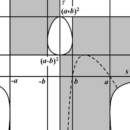
1 ∘ ) τ = ( a + b ) 2 , s ∈ [ − a , 0 ) ∪ [ b , + ∞ ) ; 2 ∘ ) τ = ( a − b ) 2 , s ∈ [ − a , − b ] ∪ ( 0 , + ∞ ) ; 3 ∘ ) s = − a , τ ⩾ ( a − b ) 2 ; 4 ∘ ) s = − b , τ ⩾ ( a − b ) 2 ; 5 ∘ ) s = b , τ ⩽ ( a + b ) 2 ; 6 ∘ ) s = a , τ ⩽ ( a + b ) 2 ; 7 ∘ ) τ = 0 , s ∈ ( 0 , + ∞ ) ; 8 ∘ ) τ = ( a 2 − s 2 + b 2 − s 2 ) 2 , s ∈ [ − b , 0 ) ; 9 ∘ ) τ = ( a 2 − s 2 − b 2 − s 2 ) 2 , s ∈ ( 0 , b ] ; 10 ∘ ) τ = − ( s 2 − a 2 − s 2 − b 2 ) 2 , s ∈ [ a , + ∞ ) . \begin{array}[]{l}\;1^{\circ})\;\tau=(a+b)^{2},\;s\in[-a,0)\cup[b,+\infty);\\
\;2^{\circ})\;\tau=(a-b)^{2},\;s\in[-a,-b]\cup(0,+\infty);\\
\;3^{\circ})\;s=-a,\;\tau\geqslant(a-b)^{2};\\
\;4^{\circ})\;s=-b,\;\tau\geqslant(a-b)^{2};\\
\;5^{\circ})\;s=b,\;\tau\leqslant(a+b)^{2};\\
\;6^{\circ})\;s=a,\;\tau\leqslant(a+b)^{2};\\
\;7^{\circ})\;\tau=0,\;s\in(0,+\infty);\\
\;8^{\circ})\;\tau=(\sqrt{a^{2}-s^{2}}+\sqrt{b^{2}-s^{2}})^{2},\;s\in[-b,0);\\
\;9^{\circ})\;\tau=(\sqrt{a^{2}-s^{2}}-\sqrt{b^{2}-s^{2}})^{2},\;s\in(0,b];\\
10^{\circ})\;\tau=-(\sqrt{s^{2}-a^{2}}-\sqrt{s^{2}-b^{2}})^{2},\;s\in[a,+\infty).\end{array}
Theorem 4 .
The solutions of the system (1.1 under the conditions
(1.12 exist iff the constants of the first integrals
(2.13 , (2.16 satisfy one of the
following
1 ∘ ) − a ⩽ s ⩽ − b , τ ⩾ ( a − b ) 2 ; 2 ∘ ) − b ⩽ s < 0 , τ ⩾ ( a 2 − s 2 + b 2 − s 2 ) 2 ; 3 ∘ ) 0 < s ⩽ b , τ ⩽ ( a 2 − s 2 − b 2 − s 2 ) 2 ; 4 ∘ ) b ⩽ s ⩽ a , τ ⩽ ( a + b ) 2 ; 5 ∘ ) s ⩾ a , − ( s 2 − b 2 − s 2 − a 2 ) 2 ⩽ τ ⩽ ( a + b ) 2 . \begin{array}[]{l}1^{\circ})\;-a\leqslant s\leqslant-b,\;\tau\geqslant(a-b)^{2};\\
2^{\circ})\;-b\leqslant s<0,\;\tau\geqslant(\sqrt{\mathstrut a^{2}-s^{2}}+\sqrt{\mathstrut b^{2}-s^{2}})^{2};\\
3^{\circ})\;\;0<s\leqslant b,\;\tau\leqslant(\sqrt{\mathstrut a^{2}-s^{2}}-\sqrt{\mathstrut b^{2}-s^{2}})^{2};\\
4^{\circ})\;\;b\leqslant s\leqslant a,\;\tau\leqslant(a+b)^{2};\\
5^{\circ})\;\;s\geqslant a,\;-(\sqrt{\mathstrut s^{2}-b^{2}}-\sqrt{\mathstrut s^{2}-a^{2}})^{2}\leqslant\tau\leqslant(a+b)^{2}.\end{array}
The complete proof of these statements is purely technical (see
[10 ] ) and contains the scrupulous analysis of the regions on
the ( x , ξ ) 𝑥 𝜉 (x,\xi) 5.2 5.3 [11 ] for the pair ( S , H ) 𝑆 𝐻 (S,H) 𝔒 𝔒 \mathfrak{O} rank ( H × K × G ) < 2 rank 𝐻 𝐾 𝐺 2 {\rm{rank}}\,(H\times K\times G)<2
Figure 1: The admissible region in the ( s , τ ) 𝑠 𝜏 (s,\tau)
The admissible region is shaded in Fig.1. The dense lines and curves
represent the equations of the bifurcation diagram, the dashed curve
illustrates the equation (4.11
6 Separation of variables
In the sequel we suppose that τ σ ≠ 0 𝜏 𝜎 0 \tau\sigma\neq 0 τ = 0 𝜏 0 \tau=0 2.18 ( 2 g − p 2 h ) 2 = r 4 k superscript 2 𝑔 superscript 𝑝 2 ℎ 2 superscript 𝑟 4 𝑘 {(2g-p^{2}h)^{2}=r^{4}k} 𝔑 𝔑 \mathfrak{N} [9 ] . The equations of motion on
𝔑 𝔑 \mathfrak{N} [8 ] .
If σ = 0 𝜎 0 \sigma=0 2.18 1.11 1.9 𝔒 𝔒 \mathfrak{O} 1.10
Considering the second equation (3.21 μ = | r 2 x 1 − τ y 1 | = | r 2 x 2 − τ y 2 | 𝜇 superscript 𝑟 2 subscript 𝑥 1 𝜏 subscript 𝑦 1 superscript 𝑟 2 subscript 𝑥 2 𝜏 subscript 𝑦 2 \mu=|r^{2}x_{1}-\tau y_{1}|=|r^{2}x_{2}-\tau y_{2}|
μ 2 = τ ξ 2 + σ x 2 − τ σ . superscript 𝜇 2 𝜏 superscript 𝜉 2 𝜎 superscript 𝑥 2 𝜏 𝜎 \mu^{2}=\tau\xi^{2}+\sigma x^{2}-\tau\sigma. (6.1)
This equation defines the second-order surface ℳ ℳ \mathcal{M} 𝐑 3 ( x , ξ , μ ) superscript 𝐑 3 𝑥 𝜉 𝜇 {\bf R}^{3}(x,\xi,\mu) 𝔒 𝔒 \mathfrak{O} ℳ ℳ \mathcal{M}
Theorem 5 .
Supposing τ σ ≠ 0 𝜏 𝜎 0 \tau\sigma\neq 0
U = τ ξ + x μ σ ( τ − x 2 ) , V = τ ξ − x μ σ ( τ − x 2 ) . formulae-sequence 𝑈 𝜏 𝜉 𝑥 𝜇 𝜎 𝜏 superscript 𝑥 2 𝑉 𝜏 𝜉 𝑥 𝜇 𝜎 𝜏 superscript 𝑥 2 \displaystyle{U=\frac{\tau\xi+x\mu}{\sqrt{\sigma}(\tau-x^{2})},\quad V=\frac{\tau\xi-x\mu}{\sqrt{\sigma}(\tau-x^{2})}}. (6.2)
Then the equations of motion on 𝔒 𝔒 \mathfrak{O}
d U Q ( U ) − d V Q ( V ) = 0 , U d U Q ( U ) − V d V Q ( V ) = d t 2 s τ σ . formulae-sequence 𝑑 𝑈 𝑄 𝑈 𝑑 𝑉 𝑄 𝑉 0 𝑈 𝑑 𝑈 𝑄 𝑈 𝑉 𝑑 𝑉 𝑄 𝑉 𝑑 𝑡 2 𝑠 𝜏 𝜎 \displaystyle{\frac{dU}{\sqrt{Q(U)}}-\frac{dV}{\sqrt{Q(V)}}=0,\quad\frac{UdU}{\sqrt{Q(U)}}-\frac{VdV}{\sqrt{Q(V)}}=\frac{dt}{\sqrt{\mathstrut 2s\tau\sigma}}}. (6.3)
Here
Q ( w ) = ( w 2 − 1 ) ( σ w 2 − 4 s 2 χ 2 ) [ ( σ w + τ ) 2 − r 4 ] . 𝑄 𝑤 superscript 𝑤 2 1 𝜎 superscript 𝑤 2 4 superscript 𝑠 2 superscript 𝜒 2 delimited-[] superscript 𝜎 𝑤 𝜏 2 superscript 𝑟 4 Q(w)=(w^{2}-1)({\sigma}w^{2}-{4s^{2}\chi^{2}})[(\sqrt{\sigma}w+\tau)^{2}-r^{4}]. (6.4)
Proof.
Consider the local coordinates u , v 𝑢 𝑣
u,v ℳ ℳ \mathcal{M}
ξ = σ u v + 1 u + v , x = τ u − v u + v , μ = τ σ u v − 1 u + v . formulae-sequence 𝜉 𝜎 𝑢 𝑣 1 𝑢 𝑣 formulae-sequence 𝑥 𝜏 𝑢 𝑣 𝑢 𝑣 𝜇 𝜏 𝜎 𝑢 𝑣 1 𝑢 𝑣 \xi=\sqrt{\sigma}\,\frac{uv+1}{u+v},\quad x=\sqrt{\tau}\,\frac{u-v}{u+v},\quad\mu=\sqrt{\tau\sigma}\,\frac{uv-1}{u+v}. (6.5)
In addition to (3.19
σ + 2 τ ( p 2 ± r 2 ) = ( τ ± r 2 ) 2 . 𝜎 2 𝜏 plus-or-minus superscript 𝑝 2 superscript 𝑟 2 superscript plus-or-minus 𝜏 superscript 𝑟 2 2 \sigma+2\tau(p^{2}\pm r^{2})=(\tau\pm r^{2})^{2}. (6.6)
The polynomials (3.15 3.24 3.40
Φ 1 = κ φ 1 ( u ) φ 1 ( v ) , Φ 2 = κ φ 2 ( u ) φ 2 ( v ) , Ψ 1 = κ ψ 1 ( u ) ψ 2 ( v ) , Ψ 2 = κ ψ 2 ( u ) ψ 1 ( v ) , Θ 1 = κ θ 2 ( u ) θ 1 ( v ) , Θ 2 = κ θ 1 ( u ) θ 2 ( v ) , subscript Φ 1 𝜅 subscript 𝜑 1 𝑢 subscript 𝜑 1 𝑣 subscript Φ 2 𝜅 subscript 𝜑 2 𝑢 subscript 𝜑 2 𝑣 subscript Ψ 1 𝜅 subscript 𝜓 1 𝑢 subscript 𝜓 2 𝑣 subscript Ψ 2 𝜅 subscript 𝜓 2 𝑢 subscript 𝜓 1 𝑣 subscript Θ 1 𝜅 subscript 𝜃 2 𝑢 subscript 𝜃 1 𝑣 subscript Θ 2 𝜅 subscript 𝜃 1 𝑢 subscript 𝜃 2 𝑣 \begin{array}[]{ll}\displaystyle{\Phi_{1}=\kappa\,\varphi_{1}(u)\,\varphi_{1}(v)},&\displaystyle{\Phi_{2}=\kappa\,\varphi_{2}(u)\,\varphi_{2}(v),}\\[5.69054pt]
\displaystyle{\Psi_{1}=\kappa\,\psi_{1}(u)\,\psi_{2}(v)},&\displaystyle{\Psi_{2}=\kappa\,\psi_{2}(u)\,\psi_{1}(v),}\\[5.69054pt]
\displaystyle{\Theta_{1}=\kappa\,\theta_{2}(u)\,\theta_{1}(v)},&\displaystyle{\Theta_{2}=\kappa\,\theta_{1}(u)\,\theta_{2}(v),}\end{array}
where κ = 1 / ( u + v ) 2 𝜅 1 superscript 𝑢 𝑣 2 \kappa=1/(u+v)^{2}
φ 1 ( w ) = σ ( 1 + w 2 ) + 2 ( τ + r 2 ) w , φ 2 ( w ) = σ ( 1 + w 2 ) + 2 ( τ − r 2 ) w , ψ 1 ( w ) = 2 s [ ( χ + τ ) w 2 − ( χ − τ ) ] , ψ 2 ( w ) = 2 s [ ( χ − τ ) w 2 − ( χ + τ ) ] , θ 1 ( w ) = σ ( 1 − w 2 ) + 4 s τ w , θ 2 ( w ) = σ ( 1 − w 2 ) − 4 s τ w . subscript 𝜑 1 𝑤 𝜎 1 superscript 𝑤 2 2 𝜏 superscript 𝑟 2 𝑤 subscript 𝜑 2 𝑤 𝜎 1 superscript 𝑤 2 2 𝜏 superscript 𝑟 2 𝑤 subscript 𝜓 1 𝑤 2 𝑠 delimited-[] 𝜒 𝜏 superscript 𝑤 2 𝜒 𝜏 subscript 𝜓 2 𝑤 2 𝑠 delimited-[] 𝜒 𝜏 superscript 𝑤 2 𝜒 𝜏 subscript 𝜃 1 𝑤 𝜎 1 superscript 𝑤 2 4 𝑠 𝜏 𝑤 subscript 𝜃 2 𝑤 𝜎 1 superscript 𝑤 2 4 𝑠 𝜏 𝑤 \begin{array}[]{ll}\varphi_{1}(w)=\sqrt{\sigma}(1+w^{2})+2(\tau+r^{2})w,&\varphi_{2}(w)=\sqrt{\sigma}(1+w^{2})+2(\tau-r^{2})w,\\[5.69054pt]
\psi_{1}(w)=2s[(\chi+\sqrt{\tau})w^{2}-(\chi-\sqrt{\tau})],&\psi_{2}(w)=2s[(\chi-\sqrt{\tau})w^{2}-(\chi+\sqrt{\tau})],\\[5.69054pt]
\theta_{1}(w)=\sqrt{\sigma}(1-w^{2})+4s\sqrt{\tau}w,&\theta_{2}(w)=\sqrt{\sigma}(1-w^{2})-4s\sqrt{\tau}w.\end{array}
Then from (3.28 3.32
x 1 = 2 s τ r 2 [ φ 1 ( u ) φ 2 ( v ) + φ 2 ( u ) φ 1 ( v ) θ 1 ( u ) θ 1 ( v ) − θ 2 ( u ) θ 2 ( v ) ] 2 , x 2 = 2 s τ r 2 [ φ 1 ( u ) φ 2 ( v ) − φ 2 ( u ) φ 1 ( v ) θ 1 ( u ) θ 1 ( v ) + θ 2 ( u ) θ 2 ( v ) ] 2 , subscript 𝑥 1 2 𝑠 𝜏 superscript 𝑟 2 superscript delimited-[] subscript 𝜑 1 𝑢 subscript 𝜑 2 𝑣 subscript 𝜑 2 𝑢 subscript 𝜑 1 𝑣 subscript 𝜃 1 𝑢 subscript 𝜃 1 𝑣 subscript 𝜃 2 𝑢 subscript 𝜃 2 𝑣 2 subscript 𝑥 2 2 𝑠 𝜏 superscript 𝑟 2 superscript delimited-[] subscript 𝜑 1 𝑢 subscript 𝜑 2 𝑣 subscript 𝜑 2 𝑢 subscript 𝜑 1 𝑣 subscript 𝜃 1 𝑢 subscript 𝜃 1 𝑣 subscript 𝜃 2 𝑢 subscript 𝜃 2 𝑣 2 \displaystyle\begin{array}[]{l}\displaystyle{x_{1}=\frac{2s\tau}{r^{2}}\left[{\frac{\sqrt{\varphi_{1}(u)\varphi_{2}(v)}+\sqrt{\varphi_{2}(u)\varphi_{1}(v)}}{\sqrt{\theta_{1}(u)\theta_{1}(v)}-\sqrt{\theta_{2}(u)\theta_{2}(v)}}}\,\right]^{2},}\\
\displaystyle{x_{2}=\frac{2s\tau}{r^{2}}\left[{\frac{\sqrt{\varphi_{1}(u)\varphi_{2}(v)}-\sqrt{\varphi_{2}(u)\varphi_{1}(v)}}{\sqrt{\theta_{1}(u)\theta_{1}(v)}+\sqrt{\theta_{2}(u)\theta_{2}(v)}}}\,\right]^{2},}\end{array} (6.9)
y 1 = 2 s [ φ 1 ( u ) φ 2 ( v ) + φ 2 ( u ) φ 1 ( v ) ] 2 − 4 σ ( u v − 1 ) 2 [ θ 1 ( u ) θ 1 ( v ) − θ 2 ( u ) θ 2 ( v ) ] 2 , y 2 = 2 s [ φ 1 ( u ) φ 2 ( v ) − φ 2 ( u ) φ 1 ( v ) ] 2 − 4 σ ( u v − 1 ) 2 [ θ 1 ( u ) θ 1 ( v ) + θ 2 ( u ) θ 2 ( v ) ] 2 , subscript 𝑦 1 2 𝑠 superscript delimited-[] subscript 𝜑 1 𝑢 subscript 𝜑 2 𝑣 subscript 𝜑 2 𝑢 subscript 𝜑 1 𝑣 2 4 𝜎 superscript 𝑢 𝑣 1 2 superscript delimited-[] subscript 𝜃 1 𝑢 subscript 𝜃 1 𝑣 subscript 𝜃 2 𝑢 subscript 𝜃 2 𝑣 2 subscript 𝑦 2 2 𝑠 superscript delimited-[] subscript 𝜑 1 𝑢 subscript 𝜑 2 𝑣 subscript 𝜑 2 𝑢 subscript 𝜑 1 𝑣 2 4 𝜎 superscript 𝑢 𝑣 1 2 superscript delimited-[] subscript 𝜃 1 𝑢 subscript 𝜃 1 𝑣 subscript 𝜃 2 𝑢 subscript 𝜃 2 𝑣 2 \displaystyle\begin{array}[]{l}\displaystyle{y_{1}=2s\frac{\left[{{\sqrt{\varphi_{1}(u)\varphi_{2}(v)}+\sqrt{\varphi_{2}(u)\varphi_{1}(v)}}}\,\right]^{2}-4\sigma(uv-1)^{2}}{\left[{\sqrt{\theta_{1}(u)\theta_{1}(v)}-\sqrt{\theta_{2}(u)\theta_{2}(v)}}\,\right]^{2}}\,,}\\
\displaystyle{y_{2}=2s\frac{\left[{\sqrt{\varphi_{1}(u)\varphi_{2}(v)}-\sqrt{\varphi_{2}(u)\varphi_{1}(v)}}\,\right]^{2}-4\sigma(uv-1)^{2}}{\left[{\sqrt{\theta_{1}(u)\theta_{1}(v)}+\sqrt{\theta_{2}(u)\theta_{2}(v)}}\,\right]^{2}}\,,}\end{array} (6.12)
z 1 = 1 2 r ( u + v ) [ φ 1 ( u ) φ 1 ( v ) + φ 2 ( u ) φ 2 ( v ) ] , z 2 = 1 2 r ( u + v ) [ φ 1 ( u ) φ 1 ( v ) − φ 2 ( u ) φ 2 ( v ) ] . subscript 𝑧 1 1 2 𝑟 𝑢 𝑣 delimited-[] subscript 𝜑 1 𝑢 subscript 𝜑 1 𝑣 subscript 𝜑 2 𝑢 subscript 𝜑 2 𝑣 subscript 𝑧 2 1 2 𝑟 𝑢 𝑣 delimited-[] subscript 𝜑 1 𝑢 subscript 𝜑 1 𝑣 subscript 𝜑 2 𝑢 subscript 𝜑 2 𝑣 \displaystyle\begin{array}[]{c}\displaystyle{z_{1}=\frac{1}{2r(u+v)}\left[{\sqrt{\varphi_{1}(u)\varphi_{1}(v)}+\sqrt{\varphi_{2}(u)\varphi_{2}(v)}}\,\right]\,,}\\
\displaystyle{z_{2}=\frac{1}{2r(u+v)}\left[{\sqrt{\varphi_{1}(u)\varphi_{1}(v)}-\sqrt{\varphi_{2}(u)\varphi_{2}(v)}}\,\right]\,.}\end{array} (6.15)
Hence, in particular,
x 1 = 2 s τ r φ 1 ( u ) φ 2 ( v ) + φ 2 ( u ) φ 1 ( v ) θ 1 ( u ) θ 1 ( v ) − θ 2 ( u ) θ 2 ( v ) , x 2 = 2 s τ r φ 1 ( u ) φ 2 ( v ) − φ 2 ( u ) φ 1 ( v ) θ 1 ( u ) θ 1 ( v ) + θ 2 ( u ) θ 2 ( v ) . subscript 𝑥 1 2 𝑠 𝜏 𝑟 subscript 𝜑 1 𝑢 subscript 𝜑 2 𝑣 subscript 𝜑 2 𝑢 subscript 𝜑 1 𝑣 subscript 𝜃 1 𝑢 subscript 𝜃 1 𝑣 subscript 𝜃 2 𝑢 subscript 𝜃 2 𝑣 subscript 𝑥 2 2 𝑠 𝜏 𝑟 subscript 𝜑 1 𝑢 subscript 𝜑 2 𝑣 subscript 𝜑 2 𝑢 subscript 𝜑 1 𝑣 subscript 𝜃 1 𝑢 subscript 𝜃 1 𝑣 subscript 𝜃 2 𝑢 subscript 𝜃 2 𝑣 \begin{array}[]{l}\displaystyle{\sqrt{x_{1}}=\frac{\sqrt{\mathstrut 2s\,\tau}}{r}\frac{\sqrt{\varphi_{1}(u)\varphi_{2}(v)}+\sqrt{\varphi_{2}(u)\varphi_{1}(v)}}{\sqrt{\theta_{1}(u)\theta_{1}(v)}-\sqrt{\theta_{2}(u)\theta_{2}(v)}}},\\[11.38109pt]
\displaystyle{\sqrt{x_{2}}=\frac{\sqrt{\mathstrut 2s\,\tau}}{r}\frac{\sqrt{\varphi_{1}(u)\varphi_{2}(v)}-\sqrt{\varphi_{2}(u)\varphi_{1}(v)}}{\sqrt{\theta_{1}(u)\theta_{1}(v)}+\sqrt{\theta_{2}(u)\theta_{2}(v)}}}.\end{array} (6.16)
Here the arbitrary choice of sign is provided by the algebraic value
2 s τ 2 𝑠 𝜏 \sqrt{2s\tau} 3.39
x 2 w 1 = i 4 s θ 2 ( u ) θ 1 ( v ) + θ 1 ( u ) θ 2 ( v ) u + v , x 1 w 2 = i 4 s θ 2 ( u ) θ 1 ( v ) − θ 1 ( u ) θ 2 ( v ) u + v . subscript 𝑥 2 subscript 𝑤 1 𝑖 4 𝑠 subscript 𝜃 2 𝑢 subscript 𝜃 1 𝑣 subscript 𝜃 1 𝑢 subscript 𝜃 2 𝑣 𝑢 𝑣 subscript 𝑥 1 subscript 𝑤 2 𝑖 4 𝑠 subscript 𝜃 2 𝑢 subscript 𝜃 1 𝑣 subscript 𝜃 1 𝑢 subscript 𝜃 2 𝑣 𝑢 𝑣 \begin{array}[]{l}\displaystyle{\sqrt{x_{2}}w_{1}=\frac{i}{4s}\frac{\sqrt{\theta_{2}(u)\theta_{1}(v)}+\sqrt{\theta_{1}(u)\theta_{2}(v)}}{u+v}},\\[11.38109pt]
\displaystyle{\sqrt{x_{1}}w_{2}=\frac{i}{4s}\frac{\sqrt{\theta_{2}(u)\theta_{1}(v)}-\sqrt{\theta_{1}(u)\theta_{2}(v)}}{u+v}}.\end{array} (6.17)
Substitute (6.16 6.17
w 1 = i r 4 s 2 s τ [ θ 2 ( u ) θ 1 ( v ) + θ 1 ( u ) θ 2 ( v ) ] [ θ 1 ( u ) θ 1 ( v ) + θ 2 ( u ) θ 2 ( v ) ] ( u + v ) [ φ 1 ( u ) φ 2 ( v ) − φ 2 ( u ) φ 1 ( v ) ] , w 2 = i r 4 s 2 s τ [ θ 2 ( u ) θ 1 ( v ) − θ 1 ( u ) θ 2 ( v ) ] [ θ 1 ( u ) θ 1 ( v ) − θ 2 ( u ) θ 2 ( v ) ] ( u + v ) [ φ 1 ( u ) φ 2 ( v ) + φ 2 ( u ) φ 1 ( v ) ] . subscript 𝑤 1 𝑖 𝑟 4 𝑠 2 𝑠 𝜏 delimited-[] subscript 𝜃 2 𝑢 subscript 𝜃 1 𝑣 subscript 𝜃 1 𝑢 subscript 𝜃 2 𝑣 delimited-[] subscript 𝜃 1 𝑢 subscript 𝜃 1 𝑣 subscript 𝜃 2 𝑢 subscript 𝜃 2 𝑣 𝑢 𝑣 delimited-[] subscript 𝜑 1 𝑢 subscript 𝜑 2 𝑣 subscript 𝜑 2 𝑢 subscript 𝜑 1 𝑣 subscript 𝑤 2 𝑖 𝑟 4 𝑠 2 𝑠 𝜏 delimited-[] subscript 𝜃 2 𝑢 subscript 𝜃 1 𝑣 subscript 𝜃 1 𝑢 subscript 𝜃 2 𝑣 delimited-[] subscript 𝜃 1 𝑢 subscript 𝜃 1 𝑣 subscript 𝜃 2 𝑢 subscript 𝜃 2 𝑣 𝑢 𝑣 delimited-[] subscript 𝜑 1 𝑢 subscript 𝜑 2 𝑣 subscript 𝜑 2 𝑢 subscript 𝜑 1 𝑣 \begin{array}[]{l}\displaystyle{w_{1}=\frac{ir}{4s\sqrt{2s\tau}}{{\left[{\sqrt{\theta_{2}(u)\theta_{1}(v)}+\sqrt{\theta_{1}(u)\theta_{2}(v)}}\right]\left[{\sqrt{\theta_{1}(u)\theta_{1}(v)}+\sqrt{\theta_{2}(u)\theta_{2}(v)}}\right]}\over{(u+v)\left[{\sqrt{\varphi_{1}(u)\varphi_{2}(v)}-\sqrt{\varphi_{2}(u)\varphi_{1}(v)}}\right]}},}\\
\displaystyle{w_{2}=\frac{ir}{4s\sqrt{2s\tau}}{{\left[{\sqrt{\theta_{2}(u)\theta_{1}(v)}-\sqrt{\theta_{1}(u)\theta_{2}(v)}}\right]\left[{\sqrt{\theta_{1}(u)\theta_{1}(v)}-\sqrt{\theta_{2}(u)\theta_{2}(v)}}\right]}\over{(u+v)\left[{\sqrt{\varphi_{1}(u)\varphi_{2}(v)}+\sqrt{\varphi_{2}(u)\varphi_{1}(v)}}\right]}}.}\end{array} (6.18)
The axial component is found from (3.39
w 3 = i 2 2 s τ σ θ 1 ( u ) θ 2 ( u ) φ 1 ( v ) φ 2 ( v ) − φ 1 ( u ) φ 2 ( u ) θ 1 ( v ) θ 2 ( v ) ( u + v ) ( u v − 1 ) . subscript 𝑤 3 𝑖 2 2 𝑠 𝜏 𝜎 subscript 𝜃 1 𝑢 subscript 𝜃 2 𝑢 subscript 𝜑 1 𝑣 subscript 𝜑 2 𝑣 subscript 𝜑 1 𝑢 subscript 𝜑 2 𝑢 subscript 𝜃 1 𝑣 subscript 𝜃 2 𝑣 𝑢 𝑣 𝑢 𝑣 1 w_{3}=\frac{i}{2\sqrt{2s\tau\sigma}}\frac{{\sqrt{\theta_{1}(u)\theta_{2}(u)\varphi_{1}(v)\varphi_{2}(v)}-\sqrt{\varphi_{1}(u)\varphi_{2}(u)\theta_{1}(v)\theta_{2}(v)}}}{(u+v)(uv-1)}. (6.19)
Thus we have expressed all phase variables in terms of u , v 𝑢 𝑣
u,v
To obtain the differential equations for u , v 𝑢 𝑣
u,v
s 1 = x 2 + z 2 + r 2 2 x , s 2 = x 2 + z 2 − r 2 2 x . formulae-sequence subscript 𝑠 1 superscript 𝑥 2 superscript 𝑧 2 superscript 𝑟 2 2 𝑥 subscript 𝑠 2 superscript 𝑥 2 superscript 𝑧 2 superscript 𝑟 2 2 𝑥 s_{1}=\frac{x^{2}+z^{2}+r^{2}}{2x},\quad s_{2}=\frac{x^{2}+z^{2}-r^{2}}{2x}. (6.20)
The derivatives, in virtue of the system (1.8
s 1 ′ = r 2 4 x 3 ( z 1 + z 2 ) ( x 1 w 2 − x 2 w 1 ) , s 2 ′ = r 2 4 x 3 ( z 1 − z 2 ) ( x 1 w 2 + x 2 w 1 ) . formulae-sequence superscript subscript 𝑠 1 ′ superscript 𝑟 2 4 superscript 𝑥 3 subscript 𝑧 1 subscript 𝑧 2 subscript 𝑥 1 subscript 𝑤 2 subscript 𝑥 2 subscript 𝑤 1 superscript subscript 𝑠 2 ′ superscript 𝑟 2 4 superscript 𝑥 3 subscript 𝑧 1 subscript 𝑧 2 subscript 𝑥 1 subscript 𝑤 2 subscript 𝑥 2 subscript 𝑤 1 \displaystyle{s_{1}^{\prime}=\frac{r^{2}}{4x^{3}}(z_{1}+z_{2})(x_{1}w_{2}-x_{2}w_{1}),\quad s_{2}^{\prime}=\frac{r^{2}}{4x^{3}}(z_{1}-z_{2})(x_{1}w_{2}+x_{2}w_{1}).} (6.21)
On the other hand, from (6.20 6.5
s 1 = σ ( u v + 1 ) + ( τ + r 2 ) ( u + v ) 2 τ ( u − v ) , s 2 = σ ( u v + 1 ) + ( τ − r 2 ) ( u + v ) 2 τ ( u − v ) , formulae-sequence subscript 𝑠 1 𝜎 𝑢 𝑣 1 𝜏 superscript 𝑟 2 𝑢 𝑣 2 𝜏 𝑢 𝑣 subscript 𝑠 2 𝜎 𝑢 𝑣 1 𝜏 superscript 𝑟 2 𝑢 𝑣 2 𝜏 𝑢 𝑣 \displaystyle{s_{1}=\frac{\sqrt{\sigma}(uv+1)+(\tau+r^{2})(u+v)}{2\sqrt{\tau}(u-v)},}\quad\displaystyle{s_{2}=\frac{\sqrt{\sigma}(uv+1)+(\tau-r^{2})(u+v)}{2\sqrt{\tau}(u-v)},}
whence
∂ s 1 ∂ u = − φ 1 ( v ) 2 τ ( u − v ) 2 , ∂ s 1 ∂ v = φ 1 ( u ) 2 τ ( u − v ) 2 , ∂ s 2 ∂ u = − φ 2 ( v ) 2 τ ( u − v ) 2 , ∂ s 2 ∂ v = φ 2 ( u ) 2 τ ( u − v ) 2 . subscript 𝑠 1 𝑢 subscript 𝜑 1 𝑣 2 𝜏 superscript 𝑢 𝑣 2 subscript 𝑠 1 𝑣 subscript 𝜑 1 𝑢 2 𝜏 superscript 𝑢 𝑣 2 subscript 𝑠 2 𝑢 subscript 𝜑 2 𝑣 2 𝜏 superscript 𝑢 𝑣 2 subscript 𝑠 2 𝑣 subscript 𝜑 2 𝑢 2 𝜏 superscript 𝑢 𝑣 2 \begin{array}[]{ll}\displaystyle{\frac{\partial s_{1}}{\partial u}=-\frac{\varphi_{1}(v)}{2\sqrt{\tau}(u-v)^{2}},}&\displaystyle{\frac{\partial s_{1}}{\partial v}=\frac{\varphi_{1}(u)}{2\sqrt{\tau}(u-v)^{2}},}\\
\displaystyle{\frac{\partial s_{2}}{\partial u}=-\frac{\varphi_{2}(v)}{2\sqrt{\tau}(u-v)^{2}},}&\displaystyle{\frac{\partial s_{2}}{\partial v}=\frac{\varphi_{2}(u)}{2\sqrt{\tau}(u-v)^{2}}.}\end{array}
Therefore,
d u d t = 2 τ ( u − v ) 2 φ 1 ( u ) φ 2 ( v ) − φ 2 ( u ) φ 1 ( v ) [ φ 2 ( u ) d s 1 d t − φ 1 ( u ) d s 2 d t ] , d v d t = 2 τ ( u − v ) 2 φ 1 ( u ) φ 2 ( v ) − φ 2 ( u ) φ 1 ( v ) [ φ 2 ( v ) d s 1 d t − φ 1 ( v ) d s 2 d t ] . 𝑑 𝑢 𝑑 𝑡 2 𝜏 superscript 𝑢 𝑣 2 subscript 𝜑 1 𝑢 subscript 𝜑 2 𝑣 subscript 𝜑 2 𝑢 subscript 𝜑 1 𝑣 delimited-[] subscript 𝜑 2 𝑢 𝑑 subscript 𝑠 1 𝑑 𝑡 subscript 𝜑 1 𝑢 𝑑 subscript 𝑠 2 𝑑 𝑡 𝑑 𝑣 𝑑 𝑡 2 𝜏 superscript 𝑢 𝑣 2 subscript 𝜑 1 𝑢 subscript 𝜑 2 𝑣 subscript 𝜑 2 𝑢 subscript 𝜑 1 𝑣 delimited-[] subscript 𝜑 2 𝑣 𝑑 subscript 𝑠 1 𝑑 𝑡 subscript 𝜑 1 𝑣 𝑑 subscript 𝑠 2 𝑑 𝑡 \begin{array}[]{l}\displaystyle{\frac{du}{dt}=\frac{2\sqrt{\tau}(u-v)^{2}}{\varphi_{1}(u)\varphi_{2}(v)-\varphi_{2}(u)\varphi_{1}(v)}[\varphi_{2}(u)\frac{ds_{1}}{dt}-\varphi_{1}(u)\frac{ds_{2}}{dt}],}\\[11.38109pt]
\displaystyle{\frac{dv}{dt}=\frac{2\sqrt{\tau}(u-v)^{2}}{\varphi_{1}(u)\varphi_{2}(v)-\varphi_{2}(u)\varphi_{1}(v)}[\varphi_{2}(v)\frac{ds_{1}}{dt}-\varphi_{1}(v)\frac{ds_{2}}{dt}].}\end{array} (6.22)
Substitute the values (6.15 6.17 6.21 6.22
f ( u , v ) d u d t = φ 1 ( u ) φ 2 ( u ) θ 1 ( u ) θ 2 ( u ) 2 u 2 s τ σ , f ( u , v ) d v d t = φ 1 ( v ) φ 2 ( v ) θ 1 ( v ) θ 2 ( v ) 2 v 2 s τ σ , formulae-sequence 𝑓 𝑢 𝑣 𝑑 𝑢 𝑑 𝑡 subscript 𝜑 1 𝑢 subscript 𝜑 2 𝑢 subscript 𝜃 1 𝑢 subscript 𝜃 2 𝑢 2 𝑢 2 𝑠 𝜏 𝜎 𝑓 𝑢 𝑣 𝑑 𝑣 𝑑 𝑡 subscript 𝜑 1 𝑣 subscript 𝜑 2 𝑣 subscript 𝜃 1 𝑣 subscript 𝜃 2 𝑣 2 𝑣 2 𝑠 𝜏 𝜎 \begin{array}[]{l}f(u,v)\,\displaystyle{\frac{du}{dt}=\frac{\sqrt{\mathstrut\varphi_{1}(u)\varphi_{2}(u)\,\theta_{1}(u)\,\theta_{2}(u)}}{2u\sqrt{\mathstrut 2s\,\tau\sigma}}},\quad f(u,v)\,\displaystyle{\frac{dv}{dt}=\frac{\sqrt{\mathstrut\varphi_{1}(v)\varphi_{2}(v)\,\theta_{1}(v)\,\theta_{2}(v)}}{2v\sqrt{\mathstrut 2s\,\tau\sigma}}},\end{array} (6.23)
where
f ( u , v ) = ( u − v ) ( 1 − u v ) u v = ( v + 1 v ) − ( u + 1 u ) . 𝑓 𝑢 𝑣 𝑢 𝑣 1 𝑢 𝑣 𝑢 𝑣 𝑣 1 𝑣 𝑢 1 𝑢 \displaystyle{f(u,v)=\frac{(u-v)(1-uv)}{uv}=\Bigl{(}v+\frac{1}{v}\Bigr{)}-\Bigl{(}u+\frac{1}{u}\Bigr{)}}.
The variables (6.2 u , v 𝑢 𝑣
u,v
U = 1 2 ( u + 1 u ) , V = 1 2 ( v + 1 v ) . formulae-sequence 𝑈 1 2 𝑢 1 𝑢 𝑉 1 2 𝑣 1 𝑣 U=\frac{1}{2}\Bigl{(}u+\frac{1}{u}\Bigr{)},\quad V=\frac{1}{2}\Bigl{(}v+\frac{1}{v}\Bigr{)}. (6.24)
To be definite choose u = U − U 2 − 1 𝑢 𝑈 superscript 𝑈 2 1 u=U-\sqrt{\mathstrut U^{2}-1} v = V − V 2 − 1 𝑣 𝑉 superscript 𝑉 2 1 v=V-\sqrt{\mathstrut V^{2}-1} 6.23
( U − V ) d U d t = 1 2 s τ σ Q ( U ) , ( U − V ) d V d t = 1 2 s τ σ Q ( V ) formulae-sequence 𝑈 𝑉 𝑑 𝑈 𝑑 𝑡 1 2 𝑠 𝜏 𝜎 𝑄 𝑈 𝑈 𝑉 𝑑 𝑉 𝑑 𝑡 1 2 𝑠 𝜏 𝜎 𝑄 𝑉 (U-V)\frac{dU}{dt}=\frac{1}{\sqrt{2s\,\tau\sigma}}\sqrt{Q(U)},\quad(U-V)\frac{dV}{dt}=\frac{1}{\sqrt{2s\,\tau\sigma}}\sqrt{Q(V)} (6.25)
with the polynomial (6.4 6.3
To reveal the connection of Theorem 5 6.4 Q ( w ) 𝑄 𝑤 Q(w) Q ′ ( w ) superscript 𝑄 ′ 𝑤 Q^{\prime}(w)
2 32 a 4 b 4 ( a 2 − b 2 ) 2 s 10 τ 12 σ 8 χ 2 ( a 2 − s 2 ) 2 ( b 2 − s 2 ) 2 . superscript 2 32 superscript 𝑎 4 superscript 𝑏 4 superscript superscript 𝑎 2 superscript 𝑏 2 2 superscript 𝑠 10 superscript 𝜏 12 superscript 𝜎 8 superscript 𝜒 2 superscript superscript 𝑎 2 superscript 𝑠 2 2 superscript superscript 𝑏 2 superscript 𝑠 2 2 2^{32}a^{4}b^{4}(a^{2}-b^{2})^{2}s^{10}\tau^{12}\sigma^{8}\chi^{2}(a^{2}-s^{2})^{2}(b^{2}-s^{2})^{2}. (6.26)
According to (2.18 s ≠ 0 𝑠 0 s\neq 0 𝔒 𝔒 \mathfrak{O} σ = 0 𝜎 0 \sigma=0 τ = ( a ± b ) 2 𝜏 superscript plus-or-minus 𝑎 𝑏 2 \tau=(a\pm b)^{2} χ = 0 𝜒 0 \chi=0 τ = ( a 2 − s 2 ± b 2 − s 2 ) 2 𝜏 superscript plus-or-minus superscript 𝑎 2 superscript 𝑠 2 superscript 𝑏 2 superscript 𝑠 2 2 \tau=(\sqrt{\mathstrut a^{2}-s^{2}}\pm\sqrt{\mathstrut b^{2}-s^{2}})^{2} J = S × T 𝐽 𝑆 T {J=S\times\mathrm{T}} 6.4
Note that all roots of the polynomial (6.4
φ 1 ( w ) φ 2 ( w ) θ 1 ( w ) θ 2 ( w ) subscript 𝜑 1 𝑤 subscript 𝜑 2 𝑤 subscript 𝜃 1 𝑤 subscript 𝜃 2 𝑤 \varphi_{1}(w)\varphi_{2}(w)\,\theta_{1}(w)\,\theta_{2}(w) (6.27)
defining the solutions of the system (6.23 τ > 0 𝜏 0 \tau>0 σ > 0 𝜎 0 \sigma>0 6.5 u , v 𝑢 𝑣
u,v U , V 𝑈 𝑉
U,V u , v 𝑢 𝑣
u,v s , τ 𝑠 𝜏
s,\tau 𝐑 2 \ Σ ( J ) \ superscript 𝐑 2 Σ 𝐽 {\bf R}^{2}\backslash\Sigma(J) u , v 𝑢 𝑣
u,v