Oscillatory dynamics in evolutionary games are suppressed by heterogeneous adaptation rates of players

Abstract

Game dynamics in which three or more strategies are cyclically competitive, as represented by the rock-scissors-paper game, have attracted practical and theoretical interests. In evolutionary dynamics, cyclic competition results in oscillatory dynamics of densities of individual strategists. In finite-size populations, it is known that oscillations blow up until all but one strategies are eradicated if without mutation. In the present paper, we formalize replicator dynamics with players that have different adaptation rates. We show analytically and numerically that the heterogeneous adaptation rate suppresses the oscillation amplitude. In social dilemma games with cyclically competing strategies and homogeneous adaptation rates, altruistic strategies are often relatively weak and cannot survive in finite-size populations. In such situations, heterogeneous adaptation rates save coexistence of different strategies and hence promote altruism. When one strategy dominates the others without cyclic competition, fast adaptors earn more than slow adaptors. When not, mixture of fast and slow adaptors stabilizes population dynamics, and slow adaptation does not imply inefficiency for a player.

Keywords: cyclic competition, replicator dynamics, altruism, coexistence

1 Introduction

Cyclic competition among different phenotypes is often found in nature. A minimal system of cyclic competition consists of individuals of three phenotypes. In so-called rock-scissors-paper (RSP) dynamics, R beats S, S beats P, and P beats R, hence no phenotype is entirely dominant. Examples of natural RSP dynamics include tropical marine ecosystems [Buss, 1980], color polymorphism of natural lizards [Sinervo and Lively, 1996], vertebrate ecosystems in high-arctic areas [Gilg et al., 2003], real microbial communities of Escherichia coli [Kerr et al., 2002], and various disease dynamics represented by the susceptible-infected-recovered-susceptible model or its variants [Anderson and May, 1991].

Also in evolutionary game theory, cyclic competition dynamics realized by three or more strategies often appear. In social dilemma games such as the Prisoner’s Dilemma, cyclic competition often underlies the survival of altruistic strategies subject to invasion by nonaltruistic strategies. For example, if the players can take either unconditional cooperation (ALLC) or unconditional defection (ALLD) in the Prisoner’s Dilemma, ALLD eventually prevails. However, if discriminators that use reputation of other players regarding the cooperation tendency are allowed, ALLC, ALLD, and discriminators form an RSP cycle; ALLD is stronger than ALLC, ALLC and discriminators are neutral, and discriminators are stronger than ALLD under certain conditions. Accordingly, these strategies alternately prosper in the population, which implies survival of altruistic players, namely, ALLC and discriminators [Nowak and Sigmund, 1998a, Nowak and Sigmund, 1998b]. Alternatively, if players can choose not to play the public goods games, such players called loners beat ALLD, ALLD beats ALLC, and ALLC beats loners. The elicited RSP dynamics save altruistic ALLC players, which would not survive without loners [Hauert et al., 2002a, Hauert et al., 2002b, Semmann et al., 2003]. In the iterated Prisoner’s Dilemma, a mixture of ALLC, ALLD, and tit-for-tat (TFT) constitutes RSP dynamics so that altruism survives under small mutation rates [Imhof et al., 2005]. Finally, a population of different types of strategies, each of which is based only on the last actions of players, shows periodic and chaotic oscillations of population densities associated with cyclic competition [Nowak and Sigmund, 1989a, Nowak and Sigmund, 1989b, Nowak and Sigmund, 1993, Brandt and Sigmund, 2006].

As illustrated by these examples, an important consequence of cyclically competing evolutionary dynamics is oscillations of population densities. Each strategy or phenotype alternately becomes the majority until it is devoured by its enemy. Oscillations are usually self-destructive in small populations because the finite-size effect usually drives the evolutionary dynamics to eventual dominance of one of the competing phenotypes [Taylor and Jonker, 1978, Nowak and Sigmund, 1998b, Reichenbach et al., 2006]. If the model represents a ecosystem, dominance of one species implies a loss of biodiversity. In social dilemma games, a situation in which one strategy wins cyclic competition often implies a loss of altruism; in many models, an altruistic strategy is relatively weak compared to others and beats another strategy only barely [Nowak and Sigmund, 1998b, Hauert et al., 2002b, Imhof et al., 2005].

If oscillations are stabilized or suppressed, cyclically competing strategies will coexist in a population. Oscillations can be suppressed by introduction of spatial structure such as the square lattice [Hassell et al., 1991, Tainaka, 1993, Durrett and Levin, 1998, Frean and Abraham, 2001]. In line with this, oscillation amplitudes grow as the underlying population structure transits from the regular lattice to the well-mixed population by increasing the number of long-range edges [Szabó et al., 2004, Ying et al., 2007] (see [Szabó and Fáth, 2007] for more references). Alternatively, heterogeneous contact rates of individuals suppress oscillations. In this scenario, hubs, namely, individuals with many neighbors, are more susceptible to invasion by their enemies, because hubs have many enemies in the neighborhood than non-hubs on average. Then hubs complete a state-transition cycle in shorter periods. Mixture of individuals with different oscillation periods abolishes the oscillation of the entire population density [Masuda and Konno, 2006].

An implicit assumption made by these and many other studies of cyclic competition [Szabó and Fáth, 2007] is that a focal individual is invaded by each enemy neighbor independently at a constant rate. For example, if a focal individual is in state R and it has 10 neighbors, the state of the focal individual is replaced by state P, which governs R, at a rate proportional to the number of P among the 10 neighbors. In other words, each P individual preys on each R neighbor independently at a constant rate. The contributions of different P individuals add linearly. In evolutionary games, however, the effect of each neighbor adds linearly in the sense that the aggregated payoff of the focal player over is the linear sum of the payoff obtained by playing with each neighbor. Then natural selection operates on the aggregated payoff in a nonlinear manner. Here how one player elicits state transition of another player is not straightforward.

In addition, suppression of oscillations by the heterogeneity mechanism requires that the number of contacts, or neighbors, depends on individuals [Masuda and Konno, 2006]. In the context of evolutionary games, heterogeneous contact numbers also pave the way to increased altruism [Santos and Pacheco, 2005, Santos et al., 2006]. In this situation, enhanced cooperation stems from players with many contacts, who earn more by participating in the game more often. However, how to compare aggregated payoffs of players with different numbers of participation is an unresolved issue [Masuda, 2007].

In this work, we explore how oscillations in RSP dynamics can be stabilized or suppressed in evolutionary games. To avoid the problem of the heterogeneous number of contact per player, we consider a well-mixed population and assume that the adaptation rate, but not the contact number, depends on players. Some players are quicker to copy successful strategies than others. Such heterogeneous adaptation rates are known to enhance cooperation in the evolutionary Prisoner’s Dilemma on the regular lattices and small-world networks [Kim et al., 2002, Szolnoki and Szabó, 2007]. By extending the replicator dynamics, we show that heterogeneous adaptation rates suppress oscillations of population densities in well-mixed populations. We validate our theory by numerical simulations of the RSP games and the public goods game with loners [Hauert et al., 2002a, Hauert et al., 2002b].

2 Model

2.1 Replicator dynamics

We begin with the standard replicator dynamics. Suppose that there are $m$ possible phenotypes, which we call strategies. The proportion of individuals, which we call players, with strategy $i$ in the population of $n$ players is denoted by $x_{i}$ ($1\leq i\leq m$), where $\sum_{i}x_{i}=1$ and $0\leq x_{i}\leq 1$ ($1\leq i\leq m$) are always satisfied. The fitness of strategy $i$ is denoted by $f_{i}$. The standard replicator dynamics are represented by

$$\frac{dx_{i}}{dt} = x_{i}\left(f_{i}-\sum_{j=1}^{m}f_{j}x_{j}\right)$$ (1)

$$= x_{i}\sum_{j}\left(f_{i}-f_{j}\right)x_{j},$$

where we suppress the range of $j$ when no confusion arises. Players with strategy $i$ increase in number at a rate proportional to the excess of $f_{i}$ relative to the average fitness $\sum_{j}f_{j}x_{j}$. Put another way, a player with strategy $j$ switches its strategy to strategy $i$ of a randomly picked opponent at a rate proportional to the fitness difference $f_{i}-f_{j}$, if $f_{i}-f_{j}\geq 0$. If $f_{i}-f_{j}<0$, players with strategy $i$ may switch to strategy $j$. The players are interpreted to form a well-mixed population.

We rewrite Eq. (1) as

$$\frac{dx_{i}}{dt}=x_{i}\sum_{j}G(f_{i}-f_{j})x_{j}-x_{i}\sum_{j}G(f_{j}-f_{i})x_{j},$$ (2)

where

$$G(x)=\left\{\begin{array}[]{ll}x,&(x\geq 0)\\ 0.&(x<0)\end{array}\right.$$ (3)

The first term of Eq. (2) represents the inflow of the population density to strategy $i$ and the second term represents the outflow from $i$ to other strategies. Note that

$$G(x)-G(-x)=x$$ (4)

is satisfied.

2.2 Extended replicator dynamics

We extend the standard replicator dynamics by considering a heterogeneous population of players who differ in the adaptation rate. For simplicity, we assume only two adaptation rates $\beta_{x}$ and $\beta_{y}$. The corresponding proportions of each strategy in two different subpopulations are specified by $x_{i}$ and $y_{i}$ ($1\leq i\leq m$), where $\sum_{i}x_{i}=\sum_{i}y_{i}=1$, and $0\leq x_{i},y_{i}\leq 1$ ($1\leq i\leq m$). In a homogeneous population, the adaptation rate, which is common to all the players, can be ignored by rescaling the time, as is evident in Eq. (1). With two adaptation rates, the ratio $\beta_{x}/\beta_{y}$ is an essential parameter that may alter dynamical consequences. Note that the interaction rate is common to all the players, which contrasts with Taylor and Nowak (2006).

If one strategy is more profitable than another strategy irrespective of the values of $x_{i}$ and $y_{i}$ ($1\leq i\leq m$), players that adapt more rapidly enjoy more benefits. For example, in the Prisoner’s Dilemma with ALLC and ALLD strategies only, everybody in a well-mixed population will choose ALLD. Rapidly adapting ALLC players switch to ALLD in early stages to transiently exploit slowly adapting ALLC players. However, under cyclic competition, it may not be profitable to myopically follow apparently successful others. In a long term, players may be better off by adapting slowly.

We assume that players differ only in adaptation rates and that they are well-mixed. Therefore, the total payoff of a player with strategy $i$ is equal to $f_{i}$ regardless of the adaptation rate. We represent the extended replicator dynamics as follows:

$$\frac{1}{\beta_{x}}\frac{dx_{i}}{dt} = x_{i}\left(f_{i}-\sum_{j}f_{j}x_{j}\right)+y_{i}\sum_{j}G(f_{i}-f_{j})x_{j}-x_{i}\sum_{j}G(f_{j}-f_{i})y_{j}$$ (5)

$$\frac{1}{\beta_{y}}\frac{dy_{i}}{dt} = y_{i}\left(f_{i}-\sum_{j}f_{j}y_{j}\right)+x_{i}\sum_{j}G(f_{i}-f_{j})y_{j}-y_{i}\sum_{j}G(f_{j}-f_{i})x_{j}.$$ (6)

In Eq. (5), the first term in the right-hand side represents the competition within players that have adaptation rate $\beta_{x}$. This part is identical to the standard replicator dynamics. The second term represents the transition from strategy $j$ to strategy $i$ as a result of imitating a player with the different adaptation rate, that is, $\beta_{y}$. Players with strategy $j$ and adaptation rate $\beta_{x}$, whose density is $x_{j}$, switch to strategy $i$ when they meet a player with strategy $i$ and adaptation rate $\beta_{y}$. The transition rate is proportional to $G(f_{i}-f_{j})$. Note that the transition from $j$ to $i$ such that players with strategy $i$ and adaptation rate $\beta_{x}$ are imitated is taken care of by the first term. The third term represents the rate at which players with strategy $i$ and adaptation rate $\beta_{x}$ switch to strategy $j$ when they meet a player with strategy $j$ and adaptation rate $\beta_{y}$. Equation (6) can be interpreted similarly. Equations (5) and (6) guarantee $\sum_{i}dx_{i}/dt=0$ and $\sum_{i}dy_{i}/dt=0$, so that the number of players in each subpopulation is conserved.

Cyclic competition often yields coexistence of all the relevant strategies. Interested in this phenomenon, we focus on interior equilibria, which satisfy $x_{i}>0$ ($1\leq\forall i\leq m$). In the standard replicator dynamics shown in Eq. (1), suppose that the total payoff for each strategy $f_{i}$ is linear in $x_{1}$, $x_{2}$, $\ldots$, $x_{m}$, as is the case when the payoff is defined by a payoff matrix. Then the interior equilibrium is unique and determined from $f_{1}$ $=$ $f_{2}$ $=$ $\ldots$ $=$ $f_{m}$ and $\sum_{i}x_{i}=1$ [Zeeman, 1980, Hofbauer and Sigmund, 1998]. For the extended replicator dynamics, the interior equilibrium is not unique even when $f_{i}$ is linear in the density of each strategy $x_{1}+y_{1}$, $x_{2}+y_{2}$, $\ldots$, and $x_{m}+y_{m}$. Indeed, any configuration that satisfies $f_{1}$ $=$ $f_{2}$ $=$ $\ldots$ $=$ $f_{m}$, $\sum_{i}x_{i}=1$, and $\sum_{i}y_{i}=1$ leads to $dx_{i}/dt=dy_{i}/dt=0$ in Eqs. (5) and (6) for $G$ given in Eq. (3). Because there are $2m$ unknown variables and $m+1$ equations, the equilibrium is underdetermined. Only the proportion of each strategy with different adaptation rates pooled, namely, $x_{i}+y_{i}$, is determined by the equilibrium condition.

To avoid this ambiguity, we introduce a realistic assumption for $G$. Because of bounded cognitive ability and stochastic environments, players may mimic strategies of unsuccessful others with small probabilities. This factor can be implemented by allowing $G(x)>0$ for $x<0$ [Blume, 1993, Nowak et al., 2004, Ohtsuki et al., 2006, Traulsen et al., 2006]. More specifically, we assume that $G$ is any differentiable function that satisfies $G^{\prime}(x)>0$, $\lim_{x\to-\infty}G(x)=0$, and Eq. (4). This assumption implies that $\lim_{x\to\infty}G(x)/x=\lim_{x\to\infty}(x+G(-x))/x=1$ and $G^{\prime}(0)=1/2$.

Then, it is straightforward to see that the interior equilibrium in the case of the linear payoff is uniquely given by $f_{1}$ $=$ $f_{2}$ $=$ $\ldots$ $=$ $f_{m}$, $\sum_{i}x_{i}=1$, $\sum_{i}y_{i}=1$, and $x_{i}=y_{i}$ ($1\leq i\leq m$). The uniqueness can be shown as follows. If $f_{1}$ $=$ $f_{2}$ $=$ $\ldots$ $=$ $f_{m}$ does not hold at an interior equilibrium, there exists an $i_{0}$ such that $f_{i_{0}}>\sum_{j}f_{j}x_{j}$ and $f_{i_{0}}>\sum_{j}f_{j}y_{j}$ at this point. For this $i_{0}$, summation of Eqs. (5) and (6) yields

$$0=\frac{1}{\beta_{x}}\frac{dx_{i_{0}}}{dt}+\frac{1}{\beta_{y}}\frac{dy_{i_{0}}}{dt}=x_{i_{0}}\left(f_{i_{0}}-\sum_{j}f_{j}x_{j}\right)+y_{i_{0}}\left(f_{i_{0}}-\sum_{j}f_{j}y_{j}\right)>0,$$ (7)

which is a contradiction. Therefore, $f_{1}$ $=$ $f_{2}$ $=$ $\ldots$ $=$ $f_{m}$ holds. Then the first terms in the right-hand sides of Eqs. (5) and (6) vanish, and we obtain $x_{i}=y_{i}$ ($1\leq i\leq m$).

3 Analysis of the RSP games

We consider the symmetric RSP game whose fitness $f_{i}$ is specified via the following payoff matrix:

$$A=\left(\begin{array}[]{ccc}0&-a_{2}&b_{3}\\ b_{1}&0&-a_{3}\\ -a_{1}&b_{2}&0\end{array}\right)$$ (8)

[Zeeman, 1980, Hofbauer and Sigmund, 1998]. Each player can take one of the three strategies ($m=3$), and the row player and the column player correspond to the focal player and the opponent, respectively.

The unique interior equilibrium of the extended replicator dynamics is given by

$$\left(\begin{array}[]{c}x_{1}^{*}\\ x_{2}^{*}\\ x_{3}^{*}\end{array}\right)=\left(\begin{array}[]{c}y_{1}^{*}\\ y_{2}^{*}\\ y_{3}^{*}\end{array}\right)=\frac{1}{\Sigma}\left(\begin{array}[]{c}a_{2}a_{3}+a_{3}b_{2}+b_{2}b_{3}\\ a_{1}a_{3}+a_{1}b_{3}+b_{1}b_{3}\\ a_{1}a_{2}+a_{2}b_{1}+b_{1}b_{2}\end{array}\right),$$ (9)

where $\Sigma$ is the normalization constant. In the standard replicator dynamics, this equilibrium is asymptotically stable when $a_{1}a_{2}a_{3}<b_{1}b_{2}b_{3}$ [Zeeman, 1980, Hofbauer and Sigmund, 1998]. If $a_{1}a_{2}a_{3}>b_{1}b_{2}b_{3}$, the equilibrium is unstable, and in a finite population, the population density oscillates with ever increasing amplitudes until the population consists entirely of a single strategy. The relation $a_{1}a_{2}a_{3}=b_{1}b_{2}b_{3}$ stipulates a borderline situation in which the interior equilibrium is neutrally stable.

By a one-to-one mapping of the population density vector, the payoff matrix $A$ can be transformed to the following form [Zeeman, 1980, Hofbauer and Sigmund, 1998]:

$$A^{\prime}=\left(\begin{array}[]{ccc}0&-a_{2}&a_{1}+\epsilon\\ a_{2}+\epsilon&0&-a_{3}\\ -a_{1}&a_{3}+\epsilon&0\end{array}\right)$$ (10)

Now, the asymptotic stability of the interior equilibrium is equivalent to $\epsilon>0$.

To show that heterogeneous adaptation rates stabilize the interior equilibrium, we even simplify Eq. (10) by setting $a_{1}=a_{2}=a_{3}=1$ [Zeeman, 1980]:

$$A^{\prime\prime}=\left(\begin{array}[]{ccc}0&-1&1+\epsilon\\ 1+\epsilon&0&-1\\ -1&1+\epsilon&0\end{array}\right)$$ (11)

The interior equilibrium is now given by

$$\left(\begin{array}[]{c}x_{1}^{*}\\ x_{2}^{*}\\ x_{3}^{*}\end{array}\right)=\left(\begin{array}[]{c}y_{1}^{*}\\ y_{2}^{*}\\ y_{3}^{*}\end{array}\right)=\frac{1}{3}\left(\begin{array}[]{c}1\\ 1\\ 1\end{array}\right),$$ (12)

which is asymptotically stable if and only if $\epsilon>0$. When $\epsilon=0$, the equilibrium is neutrally stable, with $A^{\prime\prime}$ defining a zerosum game. The standard replicator dynamics for $\epsilon=0$ becomes the most famous RSP dynamics:

$$\frac{dx_{1}}{dt} = x_{1}(x_{3}-x_{2}),$$ (13)

$$\frac{dx_{2}}{dt} = x_{2}(x_{1}-x_{3}),$$ (14)

$$\frac{dx_{3}}{dt} = x_{3}(x_{2}-x_{1}).$$ (15)

For $A^{\prime\prime}$ given in Eq. (11), we obtain

$$f_{1} = (1+\epsilon)(x_{3}+y_{3})-(x_{2}+y_{2}),$$ (16)

$$f_{2} = (1+\epsilon)(x_{1}+y_{1})-(x_{3}+y_{3}),$$ (17)

$$f_{3} = (1+\epsilon)(x_{2}+y_{2})-(x_{1}+y_{1}).$$ (18)

We linearize the extended replicator dynamics around the interior equilibrium by setting $x_{i}=x_{i}^{*}+\Delta x_{i}$, $y_{i}=y_{i}^{*}+\Delta y_{i}$ ($1\leq i\leq 3$), where $\Delta x_{i}$ and $\Delta y_{i}$ are small. Using $\Delta x_{1}+\Delta x_{2}+\Delta x_{3}=\Delta y_{1}+\Delta y_{2}+\Delta y_{3}=0$ and $G^{\prime}(0)=1/2$, we obtain

$$\frac{1}{\beta_{x}}\frac{d\Delta x_{1}}{dt}$$ (19)

$$= \left(\frac{1}{3}+\Delta x_{1}\right)\left[\left(1+\epsilon\right)\left(\Delta x_{3}+\Delta y_{3}\right)-\left(\Delta x_{2}+\Delta y_{2}\right)\right.$$

$$- \left.\epsilon\left(\Delta x_{1}+\Delta x_{2}+\Delta x_{3}\right)-\frac{\epsilon}{3}\left(\Delta y_{1}+\Delta y_{2}+\Delta y_{3}\right)\right]$$

$$+ \left(\frac{1}{3}+\Delta y_{1}\right)\sum_{j}\left[G\left(0\right)+G^{\prime}\left(0\right)\left(\Delta f_{1}-\Delta f_{j}\right)\right]\left(\frac{1}{3}+\Delta x_{j}\right)$$

$$- \left(\frac{1}{3}+\Delta x_{1}\right)\sum_{j}\left[G\left(0\right)+G^{\prime}\left(0\right)\left(\Delta f_{j}-\Delta f_{1}\right)\right]\left(\frac{1}{3}+\Delta y_{j}\right)$$

$$= \left[-\frac{2(1+\epsilon)}{3}-G\left(0\right)\right]\Delta x_{1}-\frac{2(2+\epsilon)}{3}\Delta x_{2}$$

$$+\left[-\frac{2(1+\epsilon)}{3}+G\left(0\right)\right]\Delta y_{1}-\frac{2(2+\epsilon)}{3}\Delta x_{2},$$

where $\Delta f_{i}$ is perturbation of the steady-state $f_{i}$ that originates from $\Delta x_{1}$, $\Delta x_{2}$, and $\Delta x_{3}$. By doing similar calculations for $\Delta x_{2}$, $\Delta y_{1}$, and $\Delta y_{2}$, we obtain the linear dynamics around the equilibrium given by Eq. (12) as follows:

$$\frac{d}{dt}\left(\begin{array}[]{c}\Delta x_{1}\\ \Delta x_{2}\\ \Delta y_{1}\\ \Delta y_{2}\end{array}\right)=\left(\begin{array}[]{cccc}-(1+\epsilon)B_{x}-C_{x}&-(2+\epsilon)B_{x}&-(1+\epsilon)B_{x}+C_{x}&-(2+\epsilon)B_{x}\\ (2+\epsilon)B_{x}&B_{x}-C_{x}&(2+\epsilon)B_{x}&B_{x}+C_{x}\\ -(1+\epsilon)B_{y}+C_{y}&-(2+\epsilon)B_{y}&-(1+\epsilon)B_{y}-C_{y}&-(2+\epsilon)B_{y}\\ (2+\epsilon)B_{y}&B_{y}+C_{y}&(2+\epsilon)B_{y}&B_{y}-C_{y}\end{array}\right)\left(\begin{array}[]{c}\Delta x_{1}\\ \Delta x_{2}\\ \Delta y_{1}\\ \Delta y_{2}\end{array}\right),$$ (20)

where $B_{x}=2\beta_{x}/3$, $B_{y}=2\beta_{y}/3$, $C_{x}=\beta_{x}G(0)$, and $C_{y}=\beta_{y}G(0)$. Noting that $B_{x}C_{y}=B_{y}C_{x}$, we obtain the following eigenvalue equation:

$$\lambda^{4}+\left[2\left(C_{x}+C_{y}\right)+\epsilon\left(B_{x}+B_{y}\right)\right]\lambda^{3}$$ (21)

$$+ \left[\left(3+3\epsilon+\epsilon^{2}\right)\left(B_{x}^{2}+B_{y}^{2}\right)+\left(C_{x}+C_{y}\right)^{2}+\left(6+6\epsilon+\epsilon^{2}\right)B_{x}B_{y}\right.$$

$$+ \left.\epsilon\left(B_{x}C_{x}+B_{y}C_{y}+3B_{x}C_{y}+3B_{y}C_{x}\right)\right]\lambda^{2}$$

$$+ \left[6\left(2+\epsilon\right)^{2}B_{x}B_{y}\left(C_{x}+C_{y}\right)+4\epsilon\left(B_{x}+B_{y}\right)C_{x}C_{y}\right]\lambda+12(2+\epsilon)^{2}B_{x}B_{y}C_{x}C_{y}=0.$$

The interior equilibrium is stable if all the solutions of Eq. (21) have negative real parts. The Routh-Hurwitz criteria dictate that all the eigenvalues of Eq. (21) are negative if and only if the four principal minors of a matrix calculated from the coefficients of Eq. (21) are all positive. To the first order of $\epsilon$, the principal minors are calculated as:

$$|H_{1}| = 2(C_{x}+C_{y})+\epsilon(B_{x}+B_{y}),$$ (22)

$$|H_{2}| = 6(1+\epsilon)\left(B_{x}-B_{y}\right)^{2}(C_{x}+C_{y})+2\left(C_{x}+C_{y}\right)^{3}+3\epsilon(B_{x}+B_{y})^{3}$$ (23)

$$+ \epsilon(B_{x}+B_{y})(3C_{x}^{2}+10C_{x}C_{y}+3C_{y}^{2})$$

$$|H_{3}| = 144(1+2\epsilon)(B_{x}-B_{y})^{2}B_{x}B_{y}(C_{x}+C_{y})^{2}+48(1+\epsilon)B_{x}B_{y}(C_{x}+C_{y})^{2}(C_{x}-C_{y})^{2}$$ (24)

$$+ 72\epsilon(B_{x}+B_{y})^{3}B_{x}B_{y}(C_{x}+C_{y})+24\epsilon(B_{x}+B_{y})B_{x}B_{y}(C_{x}+C_{y})(2C_{x}^{2}+3C_{x}C_{y}+2C_{y})^{2}$$

$$+ 24\epsilon(B_{x}+B_{y})(B_{x}-B_{y})^{2}(C_{x}+C_{y})C_{x}C_{y}+8\epsilon(B_{x}+B_{y})(C_{x}+C_{y})^{3}C_{x}C_{y},$$

$$|H_{4}| = 48(1+\epsilon)B_{x}B_{y}C_{x}C_{y}|H_{3}|$$ (25)

These relations hold whenever $\epsilon>0$, that is, when the interior equilibrium is stable even without heterogeneous adaptation rates. When $\epsilon<0$, the interior equilibrium is unstable with homogeneous adaptation rates. In accordance, $|H_{3}|<0$ holds when $B_{x}=B_{y}>0$, $C_{x}=C_{y}>0$, and $\epsilon<0$. To make $|H_{3}|$ positive for $\epsilon<0$, the heterogeneity quantified by $(B_{x}-B_{y})^{2}$ and $(C_{x}-C_{y})^{2}$, must be large enough to compensate the negative contribution of the last four $\epsilon$ terms of Eq. (24) to $|H_{3}|$.

Although Eqs. (22)–(25) are valid for infinitesimally small $|\epsilon|$, they are exact when $\epsilon=0$. In this case, the standard replicator dynamics have a neutrally stable interior equilibrium [Zeeman, 1980, Hofbauer and Sigmund, 1998]. Actually, $|H_{3}|=0$ holds when $B_{x}=B_{y}>0$, $C_{x}=C_{y}>0$, and $\epsilon=0$. Equations (22)–(25) imply that the asymptotic stability is equivalent to $B_{x}\neq B_{y}$ and $C_{x}\neq C_{y}$, or equivalently, $\beta_{x}\neq\beta_{y}$, in addition to $\beta_{x}>0$ and $\beta_{y}>0$. These analytical results indicate that heterogeneous adaptation rates stabilize the interior equilibrium.

4 Numerical results

In this section, we perform individual-based numerical simulations in which players are involved in evolutionary games with cyclic competition. As a rule of thumb, when the population size is of the order of 100 or smaller, the finite-size effect tends to make amplitudes of oscillatory population densities explode. We show that, even in this case, introduction of heterogeneous adaptation rates prohibits the monopoly by a single strategy, which would follow unrestricted growths of oscillation amplitudes. As a result, different competing strategies can coexist. In the following numerical simulations, we assume $n=200$ players.

4.1 RSP games

Consider that players are involved in the RSP game whose payoff matrix is given by Eq. (11). Each player takes one of the three strategies. Initially, players select each strategy randomly and independently with probability $1/3$. Any pair of players is engaged in the game with probability 0.5 so that each player is matched with $0.5(n-1)=99.5$ other players on average.

In accordance with the replicator dynamics, players with larger accumulated payoffs can disseminate their strategies more successfully. We pick 40 pairs of players randomly from the population and denote one such pair by $i$ and $j$. Only player $i$ is assumed to be subject to strategy update in this pairing. Player $i$ copies player $j$’s strategy with probability $\beta_{i}(f_{j}-f_{i})$, where $\beta_{i}$ is the adaptation rate of player $i$. If $f_{i}>f_{j}$, no imitation occurs. This update rule is equivalent to the replicator dynamics with the piecewise linear $G$ given in Eq. (3). Although we required smooth $G$ for formulating extended replicator dynamics, here we use the piecewise linear $G$ for simplicity. The average adaptation rate is set equal to $\overline{\beta}=0.5/n=0.0025$, and the adaptation rate of player $i$, or $\beta_{i}$, is distributed according to the uniform density on $\left[\overline{\beta}\left(1-\Delta_{\beta}\right),\overline{\beta}\left(1+\Delta_{\beta}\right)\right]$, independently for different players. As $\Delta_{\beta}$ increases, the population becomes heterogeneous.

For $\epsilon=0$, the interior equilibrium is neutrally, but not asymptotically, stable in the standard replicator dynamics. The results of individual-based simulations are shown in Fig. 1 for three values of heterogeneity $\Delta_{\beta}$. In Fig. 1, only the proportions of players with strategy 1 (first-row players in Eq. (11)) are shown for visibility. In reality, three subpopulations, respectively, corresponding to strategies 1, 2, and 3 alternately prosper due to cyclic competition.

When $\Delta_{\beta}=0$ (Fig. 1(A)), all the players share the same adaptation rate ($\beta_{i}=\overline{\beta}$) as in the standard replicator dynamics. Owing to the finite-size effect, the oscillation grows in amplitude until one strategy dominates the population after some oscillation cycles. The proportion of strategy 1 presented in the figure reaches 0 or 1 depending on initial conditions and stochasticity in strategy updating. As the adaptation rate becomes heterogeneous, explosion of the oscillation amplitude tends to be suppressed. When $\Delta_{\beta}=0.4$ (Fig. 1(B)), oscillations persist for much longer time than when $\Delta_{\beta}=0$ (Fig. 1(A)). With more heterogeneity, the oscillation persists even longer and the oscillation amplitude becomes smaller, as shown in Fig. 1(C) for $\Delta_{\beta}=0.8$.

Precisely speaking, the theory predicts damping oscillations for heterogeneous adaptation rates, but not reverberating ripples apparent in Fig. 1(B) and (C). There are many factors that could contribute to this discrepancy: the nonsmooth $G$, more than two values of adaptation rates, stochasticity introduced by random encountering and updating of randomly selected players, and small $n$. Because the aim in the numerical simulations is to show suppression of oscillations by heterogeneity, we do not explore this subtle discrepancy.

For $\epsilon=-0.1$, the interior equilibrium is unstable in the standard replicator dynamics. In a homogeneous population, two of the three strategies are eradicated in an early stage (Fig. 2(A); $\Delta_{\beta}=0$). Even with some heterogeneity in the adaptation rate, the oscillation ends up with explosion (Fig. 2(B); $\Delta_{\beta}=0.4$). At this level of heterogeneity, coexistence generally lasts longer than the homogeneous case, whereas its duration depends pretty much on numerical runs (results not shown). With stronger heterogeneity (Fig. 2(C); $\Delta_{\beta}=0.8$), three strategies coexist stably with a high probability.

4.2 Public goods game with voluntary participation

As another numerical example, we examine the public goods game, which is a type of the multiperson Prisoner’s Dilemma. We assume that $N$ ($<n$) randomly selected players form a group. In the standard public goods game, each of $N$ players has an option to donate a unit cost or to refrain from donation. The donated amount is multiplied by $r$ and divided equally by the $N$ players. When $r>1$, donation is a prosocial action because it increases the aggregated benefit of the group by proportion $r-1$. However, a player always earns more by not donating, which is a social dilemma. In an evolutionary framework, the public goods game is repeated with different random groups in one generation. Then, the players with higher accumulated payoffs have more chances to disseminate their strategies. Without further assumptions, altruistic donation is completely overridden by defection.

Incorporation of another strategy called loner opens the way to survival of cooperators [Hauert et al., 2002a, Hauert et al., 2002b]. A loner does not participate in the game, and it gains the side payoff $\sigma>0$. The key assumption is that it is better not to play than to be in a group of defectors. If there are $N-S$ loners in a group, the other $S$ players play the public goods game. If there are $n_{c}$ cooperators among $S$ players given $S\geq 2$, the payoffs for a cooperator, defector, and loner, are equal to $f_{c}=-1+rn_{c}/S$, $f_{d}=rn_{c}/S$, and $f_{l}=\sigma$, respectively. If $S=1$, the single player constituting the group behaves like a loner because there is nobody to play the game with.

With $\sigma<r-1$, it is better to stay in a group of cooperators than not to participate. Therefore, defectors dominate cooperators, as before, and loners dominate defectors, and cooperators dominate loners, which implies the RSP relation. According to the meanfield analysis with the standard replicator equations, the coexistence equilibrium is neutrally stable [Hauert et al., 2002a, Hauert et al., 2002b]. The stable oscillation of the population density numerically shown for $n=5000$ [Hauert et al., 2002a] may collapse in small populations. Oscillations can be stabilized by placing players on the regular lattice [Szabo and Hauert 2002] or small-world networks with sufficient spatial structure [Szabó and Vukov 2004, Wu et al., 2005] (see [Szabó and Fáth, 2007] for more references). Here we are concerned to an alternative: the heterogeneity mechanism.

We perform numerical simulations with $n=200$, $N=5$, $r=3$, and $\sigma=1$. Initially, each player selects each strategy with probability $1/3$. The generation payoff of player $i$ is determined as the summation of the payoff after 2000 rounds of group formation. As in the numerical simulations of the RSP game (Sec. 4.1), 40 players are subject to strategy update at the end of each generation. The average adaptation rate is set equal to $\overline{\beta}=0.2N/n=0.005$.

The results are shown in Fig. 3 for different degrees of heterogeneity in the adaptation rate. In each panel, cooperators (thin solid lines) are devoured by defectors (thin dashed lines), defectors are devoured by loners (thick solid lines), and loners are devoured by cooperators. This completes one RSP cycle. When the adaptation rate is homogeneous as in the standard replicator dynamics, the oscillation expands due to the finite-size effect. Two of the three strategies finally disappear (Fig. 3(A); $\Delta_{\beta}=0$). Unless $r$ is so large that loners are not needed for the survival of cooperators, loners are relatively stronger than cooperators and defectors without violating the RSP relationship [Hauert et al., 2002a, Hauert et al., 2002b]. Accordingly, the strategy that dominates finite populations are usually loners, which contrasts to the case of the RSP game. When the adaptation rate is heterogeneous (Fig. 3(B); $\Delta_{\beta}=0.4$), oscillations typically last for longer time. With a stronger degree of heterogeneity (Fig. 3(C); $\Delta_{\beta}=0.8$), oscillations are more stable. In this way, heterogeneity promotes survival of cooperators in small populations of players in the Prisoner’s Dilemma.

5 Discussion

5.1 Summary of the results

We have analyzed evolutionary game dynamics of cyclically competing strategies (or phenotypes) with heterogeneous adaptation rates. We have shown analytically and numerically that such heterogeneity suppresses oscillations of the density of each strategy and dominance of a particular strategy, which often occur in standard evolutionary dynamics with cyclic competition. In a game such that a specific strategy is stable with a large attractive basin, players with large adaptation rates shift to the lucrative strategy quickly. Then they can transiently exploit conservative players with small adaptation rates. A larger adaptation rate is better in this situation. However, in games with cyclic competition, an obvious hierarchy of strategies is absent. Then conservative players contribute to diversification of a population without really sacrificing their own benefits.

The assumption that different players have different adaptation rates seems realistic. Therefore our results imply that cyclic competition does not necessarily lead to apparent oscillations of population densities or dominance of particular strategies, which many analytical models predict. The other way round, an ordinary situation where three or more types of strategists stably coexist does not exclude operation of cyclic competition that is not weak.

Generally speaking, evolutionary dynamics in finite populations deviate from theoretical predictions for infinite populations [Nowak et al., 2004]. In homogeneous populations, RSP dynamics that show stable oscillations in infinite populations usually show unstable oscillations in finite populations, so that all but one phenotypes will disappear [Reichenbach et al., 2006]. In the context of evolutionary games, altruistic strategies that are relatively weak in the RSP relation are expelled in finite populations, even if they can survive in infinite populations. The public goods game with voluntary participation investigated in Sec. 4.2 is such an example. Heterogeneity saves rare strategies particularly in small populations (up to the order of 100 players).

5.2 Oscillations induced by mutation

In addition to heterogeneous adaptation rates, there are mechanisms that sustain rare strategies in evolutionary dynamics with cyclic competition. One is spatial structure of contact networks, as explained in Sec. 1 [Hassell et al., 1991, Tainaka, 1993, Durrett and Levin, 1998, Frean and Abraham, 2001, Szabo and Hauert 2002, Szabó et al., 2004, Szabó and Vukov 2004, Wu et al., 2005, Ying et al., 2007]. Another important mechanism is mutation. No strategy dies out in the presence of mutation because mutation decreases the proportions of major strategies and increases those of rare and absent strategies. Actually, mutation establishes oscillations and is a key to altruism in the iterated Prisoner’s Dilemma with cyclically competing three strategies, that is, ALLC, ALLD, and TFT [Imhof et al., 2005].

We have neglected mutation in this work. Mutation-induced oscillations, which imply coexistence of multiple strategies, and oscillations by heterogeneous adaptation rates are consistent. When mutation creates an oscillation in otherwise nonoscillatory evolutionary dynamics, the amplitude of an oscillation is fairly large because a mutation rate is typically small. A large oscillation amplitude implies that, in most of the time, the proportion of at least one strategy is very small [Imhof et al., 2005]. With this case included, heterogeneity lessens the oscillation amplitude so that the proportion of each strategy does not fluctuate so much in time.

5.3 Heavily skewed cyclic competition makes coexistence difficult

To test our theory, we examined two numerical models in Sec. 4. One is the standard RSP game that directly corresponds to the analytical model in Sec. 3. The other is the public goods game with voluntary participation [Hauert et al., 2002a, Hauert et al., 2002b]. There are other evolutionary games in which oscillations derived from cyclic competition are observed. Examples include the Prisoner’s Dilemma with a mixture of different memory-one strategies [Nowak and Sigmund, 1989a, Nowak and Sigmund, 1989b, Nowak and Sigmund, 1993], a seminal model of indirect reciprocity [Nowak and Sigmund, 1998a, Nowak and Sigmund, 1998b], and the iterated Prisoner’s Dilemma with misimplementation of the action [Brandt and Sigmund, 2006]. In these models, three or more strategies including altruistic strategies alternately prosper in infinite well-mixed populations. By additional numerical simulations, these dynamics were examined with $200\leq n\leq 1000$ and heterogeneous adaptation rates. However, it was impossible to stabilize the oscillatory dynamics with the ranges of parameter values probed (results not shown).

We conjecture that this failure is caused by the extreme asymmetry inherent in these RSP dynamics. To illustrate, suppose a population with homogeneous adaptation rates. By symmetric RSP dynamics, we mean those defined by the payoff matrix given in Eq. (11). The corresponding dynamics of the population densities are schematically depicted in Fig. 4(A) so that the interior equilibrium is located in the center of the simplex. Each point in the simplex specifies a density profile of different strategies. A point close to the corner labeled 1, for example, corresponds to a population that contains relatively many players with strategy 1. The symmetric or quasi symmetric RSP dynamics are often employed in the context of interacting particle systems as well as evolutionary games [Tainaka, 1993, Durrett and Levin, 1998, Frean and Abraham, 2001, Szabó et al., 2004, Reichenbach et al., 2006, Ying et al., 2007]. An example of heavily asymmetric, or skewed, RSP dynamics is depicted in Fig. 4(B). To complete a cycle, the trajectory has to proceed through a narrow canal between the interior equilibrium and the heteroclinic path on which only strategies 2 and 3 exist (the bottom line of the triangle). Accordingly, the proportion of strategy 1 is close to zero for some significant time in each cycle. Such heavily skewed RSP dynamics are identified in literature [Nowak and Sigmund, 1989a, Nowak and Sigmund, 1989b] and may be widely found in evolutionary games.

Because trajectories for a population of small to intermediate size accompany considerable fluctuation, it likely hits the heteroclinic path so that the rare strategy (strategy 1 in Fig. 4(B)) perishes. If the location of the interior equilibrium and trajectories derived from an infinite-population theory are extremely skewed, oscillatory dynamics will not be realized in finite populations. Because the heterogeneous adaptation rate does not change the position of the equilibrium (see Sec. 3 and [Masuda and Konno, 2006]), heterogeneity does not widen the canal. Although mutation kicks trajectories that have fallen onto the heteroclinic path back to the interior of the simplex, the rare strategy is perpetually subject to extinction. The heterogeneity mechanism discovered here will work out for RSP dynamics that are not extremely skewed.

Figure 1: Evolutionary simulations of the zerosum RSP game in finite populations. We set $n=200$, $\epsilon=0$, and $\overline{\beta}=0.0025$. The dispersion of the adaptation rate is (A) absent ($\Delta_{\beta}=0$), (B) intermediate ($\Delta_{\beta}=0.4$), and (C) large ($\Delta_{\beta}=0.8$). For clarity, the proportion of the players of only one of the three strategies is shown in each panel. The horizontal lines indicate $1/3$.

Figure 2: Evolutionary simulations of the non-zerosum RSP game in finite populations. We set $n=200$, $\epsilon=-0.1$, $\overline{\beta}=0.0025$. The dispersion of the adaptation rate $\Delta_{\beta}$ is equal to (A) 0, (B) 0.4, and (C) 0.8.

Figure 3: Evolutionary simulations of the public goods game with voluntary participation in finite populations. We set $n=200$, $N=5$, $r=3$, $\sigma=1$, $\overline{\beta}=0.005$, and (A) $\Delta_{\beta}=0$, (B) $\Delta_{\beta}=0.4$, and (C) $\Delta_{\beta}=0.8$. The proportions of cooperators, defectors, and loners, are shown by thin solid lines, thin dashed lines, and thick solid lines, respectively.

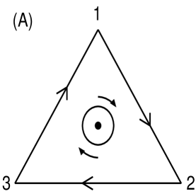
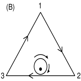
Figure 4: Schematic of trajectories of (A) symmetric and (B) heavily skewed RSP dynamics.

References

- Anderson and May, 1991 Anderson, R.M., May, R.M., 1991. Infectious Diseases of Humans. Oxford University Press, Oxford.
- Blume, 1993 Blume, L.E., 1993. The statistical mechanics of strategic interaction. Games and Economic Behavior 5, 387–424.
- Brandt and Sigmund, 2006 Brandt, H., Sigmund, K., 2006. The good, the bad and the discriminator — errors in direct and indirect reciprocity. J. Theor. Biol. 239, 183–194.
- Buss, 1980 Buss, L.W., 1980. Competitive intransitivity and size-frequency distributions of interacting populations. Proc. Natl. Acad. Sci. USA 77, 5355–5359
- Durrett and Levin, 1998 Durrett, R., Levin, S., 1998. Spatial aspects of interspecific competition. Theor. Popul. Biol. 53, 30–43.
- Frean and Abraham, 2001 Frean, M., Abraham, E.R., 2001. Rock-scissors-paper and the survival of the weakest. Proc. R. Soc. London Ser. B 268, 1323–1327.
- Gilg et al., 2003 Gilg, O., Hanski, I., Sittler, B., 2003. Cyclic dynamics in a simple vertebrate predator-prey community. Science 302, 866–868.
- Hassell et al., 1991 Hassell, M.P., Comins, H.N., May, R.M., 1991. Spatial structure and chaos in insect population dynamics. Nature 353, 255–258.
- Hofbauer and Sigmund, 1998 Hofbauer, J., Sigmund, K. 1998. Evolutionary Games and Population Dynamics. Cambridge University Press, Cambridge.
- Kerr et al., 2002 Kerr, B., Riley, M.A., Feldman, M.W., Bohannan, B.J.M., 2002. Local dispersal promotes biodiversity in a real-life game of rock-paper-scissors. Nature 418, 171–174.
- Kim et al., 2002 Kim, B.J., Trusina, A., Holme, P., Minnhagen, P., Chung, J.S., Choi, M.Y., 2002. Dynamic instabilities induced by asymmetric influence: Prisoner’s dilemma game in small-world networks. Phys. Rev. E 66, 021907.
- Hauert et al., 2002a Hauert, C., De Monte, S., Hofbauer, J., Sigmund, K., 2002a. Volunteering as red queen mechanism for cooperation in public goods games. Science 296, 1129–1132.
- Hauert et al., 2002b Hauert, C., De Monte, S., Hofbauer, J., Sigmund, K., 2002b. Replicator dynamics for optional public good games. J. Theor. Biol. 218, 187–194.
- Imhof et al., 2005 Imhof, L.A., Fudenberg, D., Nowak, M.A., 2005. Evolutionary cycles of cooperation and defection. Proc. Natl. Acad. Sci. USA 102, 10797–10800.
- Masuda and Konno, 2006 Masuda, N., Konno, N., 2006. Networks with dispersed degrees save stable coexistence of species in cyclic competition. Phys. Rev. E 74, 066102.
- Masuda, 2007 Masuda, N., 2007. Participation costs dismiss the advantage of heterogeneous networks in evolution of cooperation. Proc. R. Soc. B 274, 1815–1821.
- Nowak and Sigmund, 1989a Nowak, M., Sigmund, K., 1989a. Game dynamical aspects of the Prisoner’s Dilemma. Appl. Math. Comp. 30, 191–213.
- Nowak and Sigmund, 1989b Nowak, M., Sigmund, K. 1989b. Oscillations in the evolution of reciprocity. J. Theor. Biol. 137, 21–26.
- Nowak and Sigmund, 1993 Nowak, M., Sigmund, K., 1993. Chaos and the evolution of cooperation. Proc. Natl. Acad. Sci. USA 90, 5091–5094.
- Nowak and Sigmund, 1998a Nowak, M.A., Sigmund, K., 1998a. Evolution of indirect reciprocity by image scoring. Nature 393, 573–577.
- Nowak and Sigmund, 1998b Nowak, M.A., Sigmund, K., 1998b. The dynamics of indirect reciprocity. J. Theor. Biol. 194, 561–574.
- Nowak et al., 2004 Nowak, M.A., Sasaki, A., Taylor, C., Fudenberg, D., 2004. Emergence of cooperation and evolutionary stability in finite populations. Nature 428, 646–650.
- Ohtsuki et al., 2006 Ohtsuki, H., Hauert, C., Lieberman, E., Nowak, M.A., 2006. A simple rule for the evolution of cooperation on graphs and social networks. Nature 441, 502–505.
- Reichenbach et al., 2006 Reichenbach, T., Mobilia, M., Frey, E., 2006. Coexistence versus extinction in the stochastic cyclic Lotka-Volterra model. Phys. Rev. E 74, 051907.
- Santos and Pacheco, 2005 Santos, F.C., Pacheco, J.M., 2005. Scale-free networks provide a unifying framework for the emergence of cooperation. Phys. Rev. Lett. 95, 098104.
- Santos et al., 2006 Santos, F.C., Pacheco, J.M., Lenaerts, T., 2006. Evolutionary dynamics of social dilemmas in structured heterogeneous populations. Proc. Natl. Acad. Sci. USA 103, 3490–3494.
- Semmann et al., 2003 Semmann, D., Krambeck, H.-J., Milinski, M., 2003. Volunteering leads to rock-paper-scissors dynamics in a public goods game. Nature 425, 390–393.
- Sinervo and Lively, 1996 Sinervo, B., Lively, C.M., 1996. The rock-paper-scissors game and the evolution of alternative male strategies. Nature 380, 240–243.
- Szabo and Hauert 2002 Szabó, G., Hauert, C., 2002. Phase transitions and volunteering in spatial public goods games. Phys. Rev. Lett. 89, 118101.
- Szabó et al., 2004 Szabó, G., Szolnoki, A., Izsák, R., 2004. Rock-scissors-paper game on regular small-world networks. J. Phys. A: Math. Gen. 37, 2599–2609;
- Szabó and Vukov 2004 Szabó, G., Vukov, J., 2004. Cooperation for volunteering and partially random partnerships. Phys. Rev. E 69, 036107.
- Szabó and Fáth, 2007 Szabó, G., Fáth, G., 2007. Evolutionary games on graphs. Phys. Rep. 446, 97–216.
- Szolnoki and Szabó, 2007 Szolnoki, A., Szabó, G., 2007. Cooperation enhanced by inhomogeneous activity of teaching for evolutionary Prisoner’s Dilemma games. Europhys. Lett. 77, 30004.
- Tainaka, 1993 Tainaka, K., 1993. Paradoxical effect in a three-candidate voter model. Phys. Lett. A 176, 303–306.
- Taylor and Jonker, 1978 Taylor, P.D., Jonker, L.B., 1978. Evolutionary stable strategies and game dynamics. Math. Biosci. 40, 145–156.
- Taylor and Nowak, 2006 Taylor, C., Nowak, M.A., 2006. Evolutionary game dynamics with non-uniform interaction rates. Theor. Popul. Biol. 69, 243–252.
- Traulsen et al., 2006 Traulsen, A., Nowak, M.A., Pacheco, J.M., 2006. Stochastic dynamics of invasion and fixation. Phys. Rev. E 74, 011909.
- Wu et al., 2005 Wu, Z.-X., Xu, X.-J., Chen, Y., Wang, Y.-H., 2005. Spatial prisoner’s dilemma game with volunteering in Newman-Watts small-world networks. Phys. Rev. E 71, 037103.
- Ying et al., 2007 Ying, C.-y., Hua, D.-y., Wang, L.-y., 2007. Phase transitions for a rock-scissors-paper model with long-range-directed interactions. J. Phys. A: Math. Theor. 40, 4477–4482.
- Zeeman, 1980 Zeeman, E.C., 1980. Population dynamics from game theory. In: Lecture Notes in Mathematics, 819. Springer, New York, pp. 471–497.