The Imprints of IMBHs on the Structure of Globular Clusters: Monte-Carlo Simulations

Abstract

We present the first results of a series of Monte-Carlo simulations investigating the imprint of a central black hole on the core structure of a globular cluster. We investigate the three-dimensional and the projected density profile of the inner regions of idealized as well as more realistic globular cluster models, taking into account a stellar mass spectrum, stellar evolution and allowing for a larger, more realistic, number of stars than was previously possible with direct N-body methods. We compare our results to other N-body simulations published previously in the literature.

1 Introduction

As recently as 10 years ago, it was generally believed that black holes (BHs) occur in two broad mass ranges: stellar ($M\sim 3-20M_{\odot}$), which are produced by the core collapse of massive stars, and supermassive ($M\sim 10^{6}-10^{10}M_{\odot}$), which are believed to have formed in the center of galaxies at high redshift and grown in mass as the result of galaxy mergers (see e.g. Volonteri, Haardt & Madau 2003). However, the existence of BHs with masses intermediate between those in the center of galaxies and stellar BHs could not be established by observations up until recently, although intermediate mass BHs (IMBHs) were predicted by theory more than 30 years ago; see, e.g., Wyller (1970). Indirect evidence for IMBHs has accumulated over time from observations of so-called ultraluminous X-ray sources (ULXs), objects with fluxes that exceed the angle-averaged flux of a stellar mass BH accreting at the Eddington limit. An interesting result from observations of ULXs is that many, if not most, of them are associated with star clusters. It has long been speculated (e.g., Frank & Rees 1976) that the centers of globular clusters (GCs) may harbor BHs with masses $\sim 10^{3}\rm{M_{\odot}}$. If so, these BHs affect the distribution function of the stars, producing velocity and density cusps. A recent study by Noyola & Gebhardt (2006) obtained central surface brightness profiles for 38 Galactic GCs from HST WFPC2 images. They showed that half of the GCs in their sample have slopes for the inner 0.5” surface density brightness profiles that are inconsistent with simple isothermal cores, which may be indicative of an IMBH. However, it is challenging to explain the full range of slopes with current models. While analytical models can only explain the steepest slopes in their sample, recent N-body models of GCs containing IMBHs (Baumgardt et al. 2005), might explain some of the intermediate surface brightness slopes.

In our study we repeat some of the previous N-body simulations of GCs with central IMBHs but using the Monte-Carlo (MC) method. This gives us the advantage to model the evolution of GCs with a larger and thus more realistic number of stars. We then compare the obtained surface brightness profiles with previous results in the literature.

2 Imprints of IMBHs

The dynamical effect of an IMBH on the surrounding stellar system was first described by Peebles (1972), who argued that the bound stars in the cusp around the BH must obey a shallow power-law density distribution to account for stellar consumption near the cluster center. Analyzing the Fokker-Planck equation in energy space for an isotropic stellar distribution, Bahcall & Wolf (1976) obtained a density profile with $n(r)\propto r^{-7/4}$, which is now commonly referred to as the Bahcall-Wolf cusp. The formation of this cusp has been confirmed subsequently by many different studies using different techniques and also, more recently, by direct $N$-body methods (Baumgardt et al. 2004). In Fig. 1

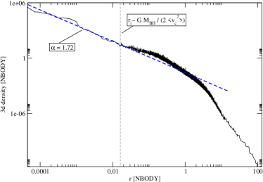
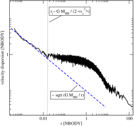
Figure 1: The imprint of an IMBH on the stellar distribution of a GC. On the left-hand side, the radial number density profile of an evolved single-mass GC is shown (solid) together with a power-law fit to its inner region (dashed line). The right hand side shows its velocity dispersion profile (solid) and the Keplerian velocity profile of the IMBH. The dotted line marks its radius of influence.

such a profile from one of our simulations is shown (for initial cluster parameters see Baumgard et al. (2004) (run16)). As can be clearly seen, the density profile of the inner region of the evolved cluster can be very well fitted by a power-law and the power-law slope $\alpha$ we obtain is, with $\alpha=1.72$, in good agreement with the value found by Bahcall & Wolf (1976). Also the extent of the cusp profile is given by the radius where the Keplerian velocity of a star around the central BH equals the velocity dispersion of the cluster core, the radius of influence of the IMBH.

However, Baumgardt et al. (2005) found that such a cusp in density might not be easily detectable in a real star cluster, as it should be much shallower and difficult to distinguish from a standard King profile. They find that this is mainly an effect of mass segregation and stellar evolution, where the more massive dark stellar remnants are concentrated towards the center while the lower-mass main sequence stars that contribute most of the light are much less centrally concentrated. In their simulations they found power-law surface brightness slopes ranging from $\alpha=-0.1$ to $\alpha=-0.3$. Based on these results they identified 9 candidate clusters from the sample of galactic GCs of Noyola & Gebhardt (2006) that might contain IMBHs. However, the disadvantage of current N-body simulations is that for realistic cluster models, that take into account stellar evolution and a realistic mass spectrum, the number of stars is restricted to typically less than $2\times 10^{5}$ as these simulations require a large amount of computing time. However, many GCs are known to be very massive, with masses reaching up to $1\times 10^{6}\rm{M_{\odot}}$ resulting in a much larger number of stars one has to deal with when modelling these objects. In previous N-body simulations, such large-N clusters have been scaled down to low-N systems. Scaling down can be achieved in two ways (e.g. Baumgardt et al. 2005): either the mass of the central IMBH $M_{BH}$ is kept constant and $N$ is decreased, effectively decreasing the total cluster mass $M_{Cl}$, or the ratio $M_{BH}/M_{Cl}$ is kept constant, while lowering both $M_{BH}$ and $M_{Cl}$. As both $M_{BH}/M_{Cl}$ and the ratio of $M_{BH}$ to stellar mass are important parameters that influence the structure of a cluster, but cannot be held constant simultaneously when lowering $N$, it is clear that only with the real $N$ a fully self-consistent simulation can be achieved. One such method that can evolve such large-$N$ systems for a sufficiently long time is the MC method.

3 Monte-Carlo Method with IMBH

The MC method shares some important properties with direct $N$-body methods, which is why it is also regarded as a randomized $N$-body scheme (see e.g. Freitag & Benz 2001). Just as direct $N$-body methods, it relies on a star-by-star description of the GC, which makes it particularly straightforward to add additional physical processes such as stellar evolution. Contrary to direct $N$-body methods, however, the stellar orbits are resolved on a relaxation time scale $T_{rel}$, which is much larger than the crossing time $t_{cr}$, the time scale on which direct $N$-body methods resolve those orbits. This change in orbital resolution is the reason why the MC method is able to evolve a GC much more efficiently than direct $N$-body methods. It achieves this efficiency, however, by making several simplifying assumptions: (i) the cluster potential has spherical symmetry (ii) the cluster is in dynamical equilibrium at all times (iii) the evolution is driven by diffusive 2-body relaxation. The specific implementation we use for our study is the MC code initially developed by Joshi et al. (2000) and further enhanced and improved by Fregau et al. (2003) and Fregau & Rasio (2007). The code is based on Hénon’s algorithm for solving the Fokker-Planck equation. It incorporates treatments of mass spectra, stellar evolution, primordial binaries, and the influence of a galactic tidal field.

The effect of an IMBH on the stellar distribution is implemented in a manner similar to Freitag & Benz (2002). In this method the IMBH is treated as a fixed, central point mass while stars are tidally disrupted and accreted onto the IMBH whenever their periastron distances lie within the tidal radius, $R_{disr}$, of the IMBH. For a given star-IMBH distance, the velocity vectors that lead to such orbits form a so called loss-cone and stars are removed from the system and their masses are added to the BH as soon as their velocity vectors enter this region. However, as the star’s removal happens on an orbital time-scale one would need to use time-steps as short as the orbital period of the star in order to treat the loss-cone effects in the most accurate fashion. This would, however, slow down the whole calculation considerably. Instead, during one MC time-step a star’s orbital evolution is followed by simulating the random-walk of its velocity vector, which approximates the effect of relaxation on the much shorter orbital time-scale. After each random-walk step the star is checked for entry into the loss-cone. For further details see Freitag & Benz (2002). Comparison with $N$-body calculations have shown that in order to achieve acceptable agreement between the two methods, the MC time-step must be chosen rather small relative to the local relaxation time, with $dt\leq 0.01T_{rel}(r)$ (Freitag et al. 2006). While choosing such a small time-step was still feasible in the code of Freitag & Benz (2002), to enforce such a criterion for all stars in our simulation would lead to a dramatic slow-down of our code and notable spurious relaxation. The reason is that our code uses a shared time step scheme, with the time-step chosen to be the smallest value of all $dt_{i}=f~{}T_{rel}(r_{i})$, where $f$ is some constant fraction and the subscript $i$ refers to the individual star. In Freitag & Benz (2002) each star is evolved separately according to its local relaxation time, allowing for larger time steps for stars farther out in the cluster where the relaxation times are longer. In order to reduce the effect of spurious relaxation we are forced to choose a larger $f$, typically around $f=0.1$. This has the consequence that the time-step criterion is only strictly fulfilled for stars typically outside of $0.1r_{h}$, where $r_{h}$ is the half-mass radius of the cluster. To arrive at the correct merger rate of stars with the IMBH, despite the larger time step for the stars in the inner region, we apply the following procedure: (i) for each star $i$ with $dt>0.01T_{rel}(r_{i})$ we take $n=dt/(0.01T_{rel})$ sub-steps. (ii) during each of these sub-steps we carry out the random-walk procedure as in Freitag & Benz (2002) (iii) after each sub-step we calculate the star’s angular-momentum $J$ according to the new velocity vector (iv) we generate a new radial position according to the new J. By updating $J$ after each sub-step we approximately account for the star’s orbital diffusion in $J$ space during a full MC step, while neglecting any changes in orbital energy. This is, at least for stars with low $J$, legitimate (Shapiro & Marchant 1978), while for the other stars the error might not be significant as the orbital energy diffusion is still slower than the $J$ diffusion (Frank & Rees 1976). A further assumption is that the cluster potential in the inner cluster region does not change significantly during a full MC step, which constrains the MC step size.

4 Comparison to N-body Simulations

In Fig. 2

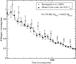
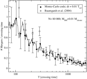
Figure 2: Comparison of the stellar merger rate per crossing time with simulations of Baumgard et al. (2004). In both cases the evolution of single-mass clusters were calculated and the tidal radius of the IMBH was fixed to $1\times 10^{-7}$ in N-body units. Full circles with error bars are results from our MC runs at selected times, while the solid line goes through all obtained points.

the rates of stellar mergers with the central BH per crossing time from two of our single-mass cluster simulations are compared to the corresponding results of Baumgardt et al. (2004) (run16 and run2). As can bee seen, the differences between our MC and the $N$-body results are within the respective error bars and thus in reasonable agreement with each other. However, the merger rates in the left panel of Fig. 2 seem to be consistently lower than in the $N$-body calculations. This might indicate that the agreement gets worse for other $M_{BH}/M_{Cl}$ than we considered here ($0.25\%-1\%$) and a different choice of time-step parameters for our MC code might be necessary in those cases. On the other hand, the differences might also be caused by differences in the initial relaxation phase before the cluster reaches an equilibrium state. This phase cannot be adequately modeled with a MC code because the code assumes dynamical equilibrium. Further comparisons to $N$-body simulations for different $M_{BH}/M_{Cl}$ and $N$ are necessary to test the validity of our method.

5 Realistic Cluster Models

In order to compare our simulations to observed GCs additional physical processes need to be included. Here we consider two clusters containing $1.3\times 10^{5}$ and $2.6\times 10^{5}$ stars with a Kroupa-mass-function (Kroupa 2001), and follow the evolution of the single stars with the code of Belczynski et al. (2002) (for all other parameter see Baumgardt et al. 2005). Fig. 3

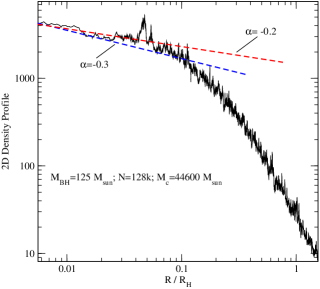
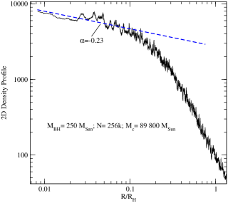
Figure 3: Two-dimensional density profile of bright stars for two clusters with different numbers of stars and BH to cluster mass ratios. The dashed line in the right panel is a power-law fit to the inner region of the cluster, while the two dashed lines in the left panel are for orientation only.

shows the two-dimensional density profiles of bright stars for the two clusters at an age of $12\rm{Gyr}$. The profile in the left panel can directly be compared to the corresponding result of Baumgardt et. al (2005) as $N$ is the same. As was expected from the discussion in §2, the profile shows only a very shallow cusp with a power-law slope $\alpha$ between $-0.2$ and $-0.3$, consistent with the $N$-body results. The right panel shows the resulting profile for a cluster that is similar but twice as massive and, consequently, has twice as many stars as in the $N$-body simulation. We obtain a very similar profile with $\alpha=-0.23$ which is very close to the average $\alpha=-0.25$ found in Baumgardt et al. (2005). Therefore, based on these very preliminary results, there seems to be no significant difference in cusp slopes for larger-$N$ clusters compared to small-$N$ ones, which means that no new candidate cluster from the sample of Noyola & Gebhardt (2006) can be identified in addition to those found by Baumgardt et al. (2005). However, the parameter space must be explored much further in order to confirm this finding.

This work was supported by NSF Grant AST-0607498 at Northwestern University.

References

- [Bahcall & Wolf(1976)] Bahcall, J. N., & Wolf, R. A. 1976, ApJ, 209, 214
- [Baumgardt et al.(2005)] Baumgardt, H., Makino, J., & Hut, P. 2005, ApJ, 620, 238
- [Baumgardt et al.(2004)] Baumgardt, H., Makino, J., & Ebisuzaki, T. 2004, ApJ, 613, 1133
- [Belczynski et al.(2002)] Belczynski, K., Bulik, T., & Kluźniak, W. ł. 2002, ApJ, 567, L63
- [Frank & Rees(1976)] Frank, J., & Rees, M. J. 1976, MNRAS, 176, 633
- [Fregeau & Rasio(2007)] Fregeau, J. M., & Rasio, F. A. 2007, ApJ, 658, 1047
- [Fregeau et al.(2003)] Fregeau, J. M., Gürkan, M. A., Joshi, K. J., & Rasio, F. A. 2003, ApJ, 593, 772
- [Freitag & Benz(2001)] Freitag, M., & Benz, W. 2001, A&A, 375, 711
- [Freitag & Benz(2002)] Freitag, M., & Benz, W. 2002, A&A, 394, 345
- [Freitag et al.(2006)] Freitag, M., Amaro-Seoane, P., & Kalogera, V. 2006, ApJ, 649, 91
- [Joshi et al.(2000)] Joshi, K. J., Rasio, F. A., & Portegies Zwart, S. 2000, ApJ, 540, 969
- [Kroupa(2001)] Kroupa, P. 2001, MNRAS, 322, 231
- [Noyola & Gebhardt(2006)] Noyola, E., & Gebhardt, K. 2006, AJ, 132, 447
- [Peebles(1972)] Peebles, P. J. E. 1972, ApJ, 178, 371
- [Shapiro & Marchant(1978)] Shapiro, S. L., & Marchant, A. B. 1978, ApJ, 225, 603
- [Volonteri et al.(2003)] Volonteri, M., Haardt, F., & Madau, P. 2003, ApJ, 582, 559
- [Wyller(1970)] Wyller, A. A. 1970, ApJ, 160, 443