Random Sierpinski network with scale-free small-world and modular structure

Abstract

In this paper, we define a stochastic Sierpinski gasket, on the basis of which we construct a network called random Sierpinski network (RSN). We investigate analytically or numerically the statistical characteristics of RSN. The obtained results reveal that the properties of RSN is particularly rich, it is simultaneously scale-free, small-world, uncorrelated, modular, and maximal planar. All obtained analytical predictions are successfully contrasted with extensive numerical simulations. Our network representation method could be applied to study the complexity of some real systems in biological and information fields.

1 Introduction

In the last few years, much attention has been paid to the study of complex networks as an interdisciplinary subject AlBa02 . It is now established that network science is a powerful tool in the analysis of real-life complex systems by providing intuitive and useful representations for networked systems. Many real-world natural and man-made systems have been examined from the perspective of complex network theory. Commonly cited examples include the Internet FaFaFa99 , the World Wide Web AlJeBa99 , metabolic networks JeToAlOlBa00 , protein networks in the cell JeMaBaOl01 , co-author networks Ne01a , sexual networks LiEdAmStAb01 , to name but a few. The empirical studies have uncovered the presence of several generic properties shared by a lot of real systems: power-law degree distribution BaAl99 , small-world effect including small average path length (APL) and high clustering coefficient WaSt98 , and community (modular) structure GiNe02 . These new discoveries have inspired researchers to develop a variety of techniques and models in an effort to understand or predict the behavior of real systems AlBa02 . It is still of current interest to reveal other different processes in real-life systems that may lead to above general characteristics.

In our earlier paper, we have proposed a family of deterministic networks based on the well-known Sierpinski fractals ZhZhZoChGu07 . These networks posses good topological properties observed in some real systems. However, their deterministic construction are not in line with the randomness of many real-world systems. In this paper, we present a stochastic Sierpinski gasket, in relation to which a novel network, named random Sierpinski network (RSN), is constructed. The obtained network is a maximal planar graph, it displays the general topological features of real systems: heavy-tailed degree distribution, small-world effect, and modular structure. We also obtain the degree correlations of RSN. All theoretical predictions are successfully confirmed by numerical simulations.

2 Brief introduction to Sierpinski network

In our previous work ZhZhZoChGu07 , motivated by the classic deterministic fractal, Sierpinski gasket (or Sierpinski triangle) Si15 ; Re94 , we introduce a new type of graph, called Sierpinski network. The well-known Sierpinski gasket, shown in figure 1(a), is constructed as follows Re94 : We start with an equilateral triangle, and denote this initial configuration by generation $t=0$. Then in the first generation $t=1$, the three sides of the equilateral triangle are bisected and the central triangle removed. This forms three copies of the original triangle, and the procedure is repeated indefinitely for all the new copies. In the limit of infinite $t$ generations, we obtain the famous Sierpinski gasket, whose Hausdorff dimension is $d_{f}=\ln 3/\ln 2$ Hu81 .

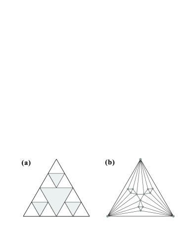
Figure 1: The first two stages of construction of the Sierpinski gasket (a) and its corresponding network (b).

From this famous fractal we have defined the Sierpinski network ZhZhZoChGu07 as illustrated in figure 1(b). The translation from the fractal to network generation is quite straightforward. Let each of the three sides of a removed triangle correspond to a node (vertex) of the network and make two nodes connected if the corresponding sides contact one another. For uniformity, the three sides of the initial equilateral triangle at step 0 also correspond to three different nodes. The resultant Sierpinski network has a power-law degree distribution $P(k)\sim k^{-\gamma}$ with $\gamma=1+\frac{\ln 3}{\ln 2}$, displays small-world effect, and is disassortative.

3 Random Sierpinski network and its iterative algorithm

In this section, we first construct a random Sierpinski gasket from the deterministic Sierpinski gasket (or Sierpinski triangle) Re94 . Then we will establish a random Sierpinski network based on the proposed stochastic fractal. Analogous to the Sierpinski triangle, the random Sierpinski gasket also starts with an equilateral triangle. At step 1, we perform a bisection of the sides and remove the downward pointing triangle forming three small copies of the original triangle. Then in each of the subsequent generations, an equilateral triangle is chosen randomly, for which bisection and removal are performed to form three small copies of it. The sketch map for the random fractal is shown in the upper panel of figure 2. From this fractal we can easily construct the random Sierpinski network with sides of the removed triangles mapped to nodes and contact to links between nodes. As in the construction of the deterministic version ZhZhZoChGu07 , the three sides of the initial equilateral triangle at step 0 are also mapped to three different nodes. Figure 2 (lower panel) shows a network derived from the random Sierpinski gasket.

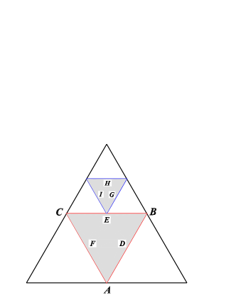
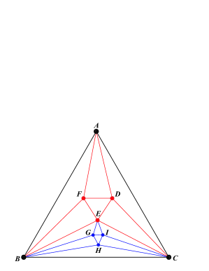
Figure 2: (Color online) The sketch maps for the construction of random Sierpinski gasket (upper panel) and its corresponding network (lower panel).

According to the construction of random Sierpinski network, we introduce a general iterative algorithm generating the network. We denote the random Sierpinski network after $t$ iterations by $W(t)$, $t\geq 0$. Initially ($t=0$), $W(0)$ has three nodes forming a triangle. At step $t=1$, we add three nodes into the original triangle. These three new nodes are connected to one another shaping a new triangle, and both ends of each edge of the new triangle are linked to a node of the original triangle. Thus we obtain $W(1)$. For $t\geq 1$, $W(t)$ is obtained from $W(t-1)$. For the convenience of description, we give the following definition: For each of the existing triangles in $W(t-1)$, if there is no nodes in its interior and among its three nodes there is only one youngest node (i.e., the other two are strictly elder than it), we call it an active triangle. At step $t-1$, we select at random an existing active triangle and replace it by the connected cluster on the right of figure 3, then $W(t)$ is produced.

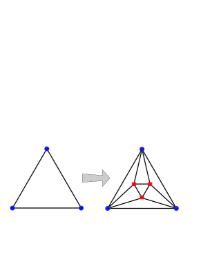
Figure 3: (Color online) Iterative construction method for the network.

Since at each time step the numbers of the nodes and edges increase by 3 and 9, respectively, we can easily know that at step $t$, the network consists of $N_{t}=3t+3$ nodes and $E_{t}=9t+3$ edges. Thus, the relation $E_{t}=3N_{t}-6$ holds for all steps. In addition, according to the connection rule, arbitrary two edges in the network never cross each other. Therefore, the considered network is a maximal planar graph We01 , which is similar to its deterministic version ZhZhZoChGu07 and some previously studied networks AnHeAnSi05 .

4 Structural characteristics

We now study the statistical properties of RSN, in terms of degree distribution, clustering coefficient, average path length, degree-degree correlations, and modularity. The analytical approaches are completely deferent from those applied to the deterministic Sierpinski network ZhZhZoChGu07 .

4.1 degree distribution

Initially ($t=0$), there is only one active triangle in the network. In the subsequent iterations, at each time step, three active triangles are created and one active triangle is deactivated simultaneously, so the total number of active triangles increases by 2. Then at time $t$, there are $2t+1$ active triangles in RSN. Note that, for an arbitrary given node, when it is born, it has a degree of 4 and one active triangle containing itself; and in the following steps, each of its two new neighbors separately generates a new active triangle involving it, and one of its existing active triangles is deactivated at the same time. So, for a node with degree $k$, the number of active triangles containing it is $\frac{k-2}{2}$. Let $N_{k}(t)$ denote the average number of nodes with degree $k$ at time $t$. By the very construction of RSN, the rate equation that accounts for the evolution of $N_{k}(t)$ with time $t$ is KaReLe00

$$\frac{dN_{k}(t)}{dt}=\frac{\frac{k-4}{2}N_{k-2}(t)-\frac{k-2}{2}N_{k}(t)}{2t+1}+3\,\delta_{k,4}.$$ (1)

The first term on the right-hand side (rhs) of Eq. (1) accounts for the process in which a node with $k-2$ links is connected to two new nodes, leading to a gain in the number of nodes with $k$ links. Since there are $N_{k-2}(t)$ nodes of degree $k-2$, such processes occur at a rate proportional to $\frac{k-4}{2}N_{k-2}(t)$, while the factor $2t+1$ converts this rate into a normalized probability. A corresponding role is played by the second (loss) term on the rhs of Eq. (1). The last term on the rhs of Eq. (1) accounts for the continuous introduction of three new nodes with degree four.

In the asymptotic limit $N_{k}(t)=(3t+3)P(k)$, where $P(k)$ is the degree distribution. Substitute this relation into Eq. (1) to lead to the following recursive equation for infinite $t$

$$P(k)=\left\{\begin{array}[]{lcl}\frac{k-4}{k+2}P(k-2)&\mbox{for}&k\geq 4+2\\ \frac{2}{3}&\mbox{for}&k=4\,,\\ \end{array}\right.$$ (2)

giving

$$P(k)=\frac{32}{k(k+2)(k-2)}.$$ (3)

In the limit of large $k$, $P(k)\sim k^{-3}$, which has the same degree exponent as the BA model BaAl99 and some hierarchical lattice models HiBe06 .

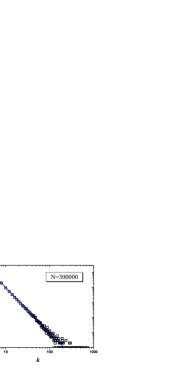
Figure 4: (Color online) Log-log graph of the degree distribution for a network with order $N=300000$. The squares denote the numerical results and the solid line shows the theoretical predication given by Eq. (3).

In order to confirm the analytical prediction, we performed numerical simulations of the network plotted in figure 4, which shows that the simulation result is well in agreement with the analytic one.

4.2 clustering coefficient

By definition, the clustering coefficient WaSt98 $C_{i}$ of node $i$ is defined as the ratio between the number of edges $e_{i}$ that actually exist among the $k_{i}$ neighbors of node $i$ and its maximum possible value, $k_{i}(k_{i}-1)/2$, i.e., $C_{i}=2e_{i}/[k_{i}(k_{i}-1)]$. Generally, in a network, for nodes with degree $k$, their clustering coefficients, $C(k)$, are not always the same. But in our network, all nodes with the same degree have identical clustering coefficient. Moreover, for a single node with degree $k$, the analytical expression for its clustering coefficient $C(k)$ can be derived exactly.

According the connection rule (see figure 3), when a node $i$ enters the system, both $k_{i}$ and $e_{i}$ are 4. In the following steps, if one of its active triangles is selected, both $k_{i}$ and $e_{i}$ increase by 2 and 3, respectively. Thus, $e_{i}$ equals to $4+\frac{3}{2}\left(k_{i}-4\right)$. The relation holds for all nodes at all steps. So one can see that there exists a one-to-one correspondence between the degree of a node and its clustering. For a node of degree $k$, we have

$$C(k)=\frac{2\,e}{k(k-1)}=\frac{2\left[4+\frac{3}{2}(k-4)\right]}{k(k-1)}=\frac{4}{k}-\frac{1}{k-1}.$$ (4)

In the limit of large $k$, $C(k)$ exhibits a power-law behavior, $C(k)\sim k^{-1}$, which has also been empirically observed in several real networks RaBa03 .

We continue to compute the average clustering coefficient $C$ of RSN by means of the clustering spectrum $C(k)$:

$$C=\sum_{k}P(k)C(k),$$ (5)

which can be easily obtained with respect to the degree distribution $P(k)$ expressed by Eq. (3). The result is

$$C = \sum_{k}\frac{32}{k(k+2)(k-2)}\left(\frac{4}{k-1}-\frac{1}{k-1}\right)$$ (6)

$$= \frac{32\ln 2}{3}-\frac{4\pi^{2}}{3}+\frac{19}{3}\approx 0.5674.$$

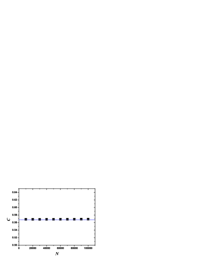
Figure 5: (Color online) Average clustering coefficient $C$ of RSN vs the network size $N$. The dotted line shows the analytic prediction and the squares denote the simulation results.

Thus the average clustering coefficient $C$ of RAN is large and independent of network size. We have performed extensive numerical simulations of the RSN. In figure 5, we present the simulation results about the average clustering coefficient of RSN, which are in complete agreement with the analytical value.

4.3 Average path length

From above discussions, we find that the existing model shows both the scale-free nature and the high clustering at the same time. In fact, our model also exhibits small-word property. Next, we will show that our network has at most a logarithmic average path length (APL) with the number of nodes. Here APL means the minimum number of edges connecting a pair of nodes, averaged over all couples of nodes.

Using an mean-field approach similar to that presented in Ref. ZhYaWa05 , one can predict the APL of our network analytically. By construction, at each time step, three nodes are added into the network. In order to distinguish different nodes, we construct a node sequence in the following way: when three new nodes are created at a given time step, we label them as $M+1,M+2,\ldots,M+3$, where $M$ is the total number of the pre-existing nodes. Eventually, every node is labeled by a unique integer, and the total number of nodes is $N_{t}=3t+3$ at time $t$.

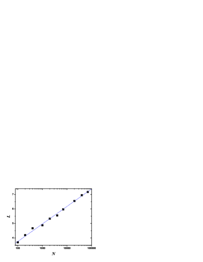
Figure 6: (Color online) Semilogarithmic plot of the average path length $L$ verse network size $N$.

We denote $L(N)$ as the APL of our network with size $N$. It follows that $L(N)=\frac{2\,D(N)}{N(N-1)}$, where $D(N)=\sum_{1\leq i<j\leq N}d_{i,j}$ is the total distance, and where $d_{i,j}$ is the smallest distance between node $i$ and $j$. Note that the distances between existing node pairs are not affected by the addition of new nodes. As in the analysis of ZhYaWa05 , we can easily derive that $D(N)\sim N^{2}\ln N$ in the infinite limit of $N$. Then, $L(N)\sim\ln N$. Thus, there is a slow growth of the APL with the network size $N$. This logarithmic scaling of $L(N)$ with network size $N$, together with the large clustering coefficient obtained in the preceding subsection, shows that the considered graph has a small-world effect. In figure 6, we report average path length $L(N)$ versus network size $N$. One can obviously see that $L(N)$ increases logarithmically with $N$.

4.4 degree correlations

First, we study the time evolution for the connectivity of an arbitrary node. Notice that the growing precess of RSN actually contains the preferential attachment mechanism, which arises in it not because of some special rule including a function of degree as in Ref. BaAl99 but naturally. Indeed, the probability that new nodes created at time $t$ will be connected to an existing node $i$ is clearly proportional to the number of active triangles containing $i$, i.e. to its $\frac{k_{i}(t)-2}{2}$. Thus a node $i$ is selected with the usual preferential attachment probability $\Pi_{i}[k_{i}(t)]=[k_{i}(t)-2]/[2(2t+1)]\sim[k_{i}(t)-2]/4t$ (for large $t$). Consequently, $k_{i}$ satisfies the dynamical equation AlBa02 :

$$\frac{\partial k_{i}(t)}{\partial t}=2\cdot\frac{k_{i}(t)-2}{4t}.$$ (7)

Considering the initial condition $k_{i}(t_{i})=4$, we have

$$k_{i}(t)=2\left(\frac{t}{i}\right)^{1/2}+2.$$ (8)

Having obtained the degrees for all nodes, we now study the degree correlations. Generally, degree correlations in a network can be conveniently measured by means of the quantity, called average nearest-neighbor degree (ANND), which is a function of node degree, and is more convenient and practical in characterizing degree-degree correlations. The ANND is defined by PaVaVe01

$$k_{nn}(k)=\sum_{k^{\prime}}k^{\prime}P(k^{\prime}|k),$$ (9)

where $P(k^{\prime}|k)$ is the condition probability that a link belonging to a node with connectivity $k$ points to a node with connectivity $k^{\prime}$. If there are no two degree correlations, $k_{nn}(k)$ is independent of $k$. When $k_{\rm nn}(k)$ increases (or decreases) with $k$, the network is said to be assortative (or disassortative) Newman02 .

Correlations can also be described by a Pearson correlation coefficient $r$, which is defined as Newman02 :

$$r=\frac{\frac{1}{M}\sum_{m}j_{m}k_{m}-\left[\frac{1}{M}\sum_{m}{\frac{1}{2}(j_{m}+k_{m})}\right]^{2}}{\frac{1}{M}\sum_{m}{\frac{1}{2}(j_{m}^{2}+k_{m}^{2})}-\left[\frac{1}{M}\sum_{m}{\frac{1}{2}(j_{m}+k_{m})}\right]^{2}}\,,$$ (10)

where $j_{m}$, $k_{m}$ are the degrees of the vertices at the ends of the $m$th edge, with $m=1,2,\cdots,M$, where $M$ denotes the number of edges in the network. The coefficient is in the range $-1\leq r\leq 1$. If the network is uncorrelated, the correlation coefficient equals zero. Disassortative networks have $r<0$, while assortative graphs have a value of $r>0$.

We can analytically calculate the function value of $k_{nn}(k)$ for the RSN. Let $R_{i}(t)$ denote the sum of the degrees of the neighbors of node $i$, evaluated at time $t$. It is represented as

$$R_{i}(t)=\sum_{j\in\Omega(i)}k_{j}(t),$$ (11)

where $\Omega(i)$ corresponds to the set of neighbors of node $i$. The ANND of node $i$ at time $t$, $k_{nn}(i,t)$, is then given by $k_{nn}(i,t)=R_{i}(t)/k_{i}(t)$. During the growth of the RSN, $R_{i}(t)$ can only increase by the addition of new nodes connected either directly to $i$, or to one of the neighbors of $i$. In the first case $R_{i}(t)$ increases by 8 (the sum of degree for two newly-created nodes), while in the second case it increases by 2. Therefore, in the continuous $k$ approximation, we can write down the following rate equation BoPa05 :

$$\frac{dR_{i}(t)}{dt} = 8\,\Pi_{i}[k_{i}(t)]+2\,\sum_{j\in\Omega(i)}\Pi_{j}[k_{j}(t)]$$ (12)

$$= \frac{2[k_{i}(t)-2]}{t}+\frac{R_{i}(t)-2k_{i}(t)}{2t}$$

$$= \frac{R_{i}(t)}{2t}+\frac{k_{i}(t)}{t}-\frac{4}{t}.$$

The general solution of Eq. (12) is

$$R_{i}(t)=4+\Phi_{0}(i)t^{\frac{1}{2}}+2\left(\frac{t}{i}\right)^{1/2}\ln t,$$ (13)

where $\Phi_{0}(i)$ is determined by the boundary condition $R_{i}(i)$. To obtain the boundary condition $R_{i}(i)$, we observe that at time $i$, the new node $i$ is connected to an existing node $j$ of degree $k_{j}(i)$ with probability $\Pi_{j}[k_{j}(i)]$, and that the degree of this node increase by 2 in the process. Thus,

$$R_{i}(i)=\sum_{j=1}^{i}\Pi_{j}[k_{j}(i)][k_{j}(i)+2]+8,$$ (14)

where the last term 8 denotes the sum of the other two new nodes created at the same time as node $i$. Inserting $\Pi_{j}[k_{j}(i)]=\frac{k_{j}(i)-2}{4i}$ and $k_{j}(i)=2\left(\frac{i}{j}\right)^{1/2}+2$ into $R_{i}(i)$ leads to

$$R_{i}(i)=8+\ln i+\sum_{j=1}^{i}2(ij)^{-\frac{1}{2}}\leq 8+3\ln i.$$ (15)

So, in the large $i$ limit, $R_{i}(i)$ is dominated by the second term, yielding

$$R_{i}(i)\lessapprox 3\ln i.$$ (16)

From here, we have

$$R_{i}(t)\simeq 2\left(\frac{t}{i}\right)^{1/2}\ln t,$$ (17)

and finally

$$k_{nn}(k,t)\simeq\ln t.$$ (18)

So, two node correlations do not depend on the degree. The ANND grows with the network size $N\approx 3t$ as $\ln N$, in the same way as in the Barabási-Albert (BA) model VapaVe02 and the two-dimensional random Apollonian network ZhZh07 .

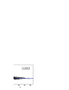
Figure 7: (Color online) Plot of average nearest-neighbor degree of the nodes with degree $k$. The squares denote the simulation results, while the solid line is the theoretical result provided by Eq. (18).

In order to confirm the validity of the obtained analytical prediction of ANND, we performed extensive numerical simulations of the RSN (see figure 7) with order $N=100002$. To reduce the effect of fluctuation on simulation results, the simulation results are average over fifty network realizations. From figure 7 we observe that for large $k$ the ANND of numerical and analytical results are in agreement with each other, while the simulated results of ANND of small $k$ have a very weak dependence on $k$, which is similar to the phenomena observed in the BA model VapaVe02 . This $k$ dependence, for small degree, cannot be detected by rate equation approach, since it has been formulated in the continuous degree $k$ approximation.

To further confirm that RSN is uncorrelated, we compute the Pearson correlation coefficient $r$ according to Eq. (10). The numerical results are reported in figure 8. From this figure, we see that for networks with small size, $r$ is negative and only a little smaller than zero; when the size of the network increases, $r$ goes to zero and is independent of size. The phenomenon of the convergence of $r$ to zero again indicates that RSN shows absence of degree correlations.

The fact that there is no degree correlation in RSN is compared with that of its deterministic variant, which shows a negative degree correlation ZhZhZoChGu07 . We guess that the reason behind this difference between RSN and its deterministic counterpart may stem from a biased choice of “active triangles”. In the evolution process of RSN, only one active triangle is updated at each iteration, while for the deterministic version, all active triangles are updated in one iteration. The difference between asynchronous and synchronous updating leads to different power-law exponents of degree distribution for the two networks, see CoRobA05 for detailed explanation. We think that the different assortative nature between the two graphs might be also related to a biased choice of active triangles at each iteration. Of course, the genuine reason for this difference requires further study.

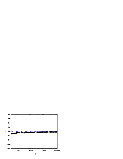
Figure 8: (Color online) Semilogarithmic graph of Pearson correlation coefficient $r$ as a function of network size $N$.

4.5 modularity

Many social and biological networks are fundamentally modular GiNe02 ; RaSoMoOlBa02 ; RaCaCeLoPa04 . These networks are formed by communities (modules) of nodes that are highly interconnected with each other, but have only a few or no links to nodes outside of the community to which they belong to. The strength of community structure is quantified through the modularity NeGi04

$$Q=\sum_{s=1}^{N_{q}}\left[\frac{l_{s}}{E}-\left(\frac{d_{s}}{2E}\right)^{2}\right],$$ (19)

where the sum runs over all communities, $N_{q}$ is the number of communities (modules), $E$ is the link number in the network, $l_{s}$ is the total number of links in the $s$th community, and $d_{s}$ is the sum of the connectivities (degrees) of the nodes in module $s$. The modularity is high if the number of within- community links is much larger than expected from chance alone.

We now look at the community structure of the network using the algorithm originally proposed by Girvan and Newman (GN) to find the partition with the largest modularity GiNe02 . The GN algorithm works by beginning with the complete network and at each step removing the edge with largest betweenness, where this quantity is recalculated after the removal of every edge. If there is more than one edge with the same largest betweenness, we remove them all at the same step. After all edges are removed, the network breaks up into $N_{t}$ communities (non-connected nodes).

Figure 9: (Color online) Modularity $Q$ as a function of number of communities $N_{q}$. The vertical dashed line indicates the best split with largest $Q$.

It is of interest to examine how the network is progressively broken into separate communities as one removes more edges. In figure 9, we present how $Q$ varies as the complete network with size $N=600$ is broken up into communities. Obviously, $Q$ has a broad large value as a function of the number of communities, showing pronounced modular structure. $Q$ is greater than 0.5 when there are between 3 and 230 communities, and the best division has $N_{q}=9$ with $Q=0.7774$. This largest value of $Q$ is in contrast to the highest values found for some real-life networks such as collaboration network of scientists. Interestingly, the combination of modular and uncorrelated properties has never been reported in previous models.

5 Conclusion

In this paper, we have introduced a stochastic Sierpinski gasket and related it to a random maximal network, called random Sierpinski network (RSN). We have also proposed a iterative algorithm generating RSN, based on which we have determined some relevant topological characteristics of the network. We have presented that the network is simultaneously scale-free, small-world, uncorrelated, and modular. Thus, the RSN successfully reproduces some remarkable properties of many natural and man-made systems. Our study provides a paradigm of representation for the complexity of many real-life systems, making it possible to study the complexity of these systems within the framework of network theory.

References

- (1) R. Albert and A.-L. Barabási, Rev. Mod. Phys. 74, 47 (2002); S. N. Dorogovtsev and J.F.F. Mendes, Adv. Phys. 51, 1079 (2002); M.E.J. Newman, SIAM Rev. 45, 167 (2003); S. Boccaletti, V. Latora, Y. Moreno, M. Chavez and D.-U. Hwanga, Phys. Rep. 424, 175 (2006).
- (2) M. Faloutsos, P. Faloutsos, C. Faloutsos, Comput. Commun. Rev. 29, 251 (1999).
- (3) R. Albert, H. Jeong, A.-L. Barabási, Nature 401, 130 (1999).
- (4) H. Jeong, B. Tombor, R. Albert, Z.N. Oltvai, A.-L. Barabási, Nature 407, 651 (2000).
- (5) H. Jeong, S. Mason, A.-L. Barabási, Z. N. Oltvai, Nature 411, 41 (2001).
- (6) M.E.J. Newman, Proc. Natl. Acad. Sci. USA 98, 404 (2001).
- (7) F. Liljeros, C.R. Edling, L.A.N. Amaral, H.E. Stanley, Y. Åberg, Nature 411, 907 (2001).
- (8) A.-L. Barabási and R. Albert, Science 286, 509 (1999).
- (9) D.J. Watts and H. Strogatz, Nature (London) 393, 440 (1998).
- (10) M. Girvan and M. E. J. Newman, Proc. Natl. Acad. Sci. U.S.A. 99, 7821 (2002).
- (11) Z. Z. Zhang, S. G. Zhou, T. Zou, L. C. Chen, and J. H. Guan, Eur. Phys. J. B 60, 259 (2007).
- (12) W. Sierpinski, Comptes Rendus (Paris) 160, 302 (1915).
- (13) C. A. Reiter, Comput. Graphics 18, 885 (1994)
- (14) S. Hutchinson, Indiana Univ. Math. J. 30, 713 (1981).
- (15) D.B. West, Introduction to Graph Theory (Prentice-Hall, Upper Saddle River, NJ, 2001).
- (16) J.S. Andrade Jr., H.J. Herrmann, R.F.S. Andrade and L.R.da Silva, Phys. Rev. Lett. 94, 018702 (2005); Z.Z. Zhang, S.G. Zhou, L.J. Fang, J.H. Guan, Y.C. Zhang, EPL (Europhys. Lett.) 79 38007 (2007); Z.Z. Zhang, F. Comellas, G. Fertin, A. Raspaud, L.L. Rong, and S. G. Zhou, J. Phys. A: Math. Thero. 41, 035004 (2008); Z.Z. Zhang, L.C. Chen, S.G. Zhou, L.J. Fang, J.H. Guan, and T. Zou, Phys. Rev. E 77, 017102 (2008).
- (17) P.L. Krapivsky, S. Redner, and F. Leyvraz, Phys. Rev. Lett. 85, 4629 (2000).
- (18) M. Hinczewski and A. N. Berker, Phys. Rev. E 73, 066126 (2006); Z. Z. Zhang, S. G. Zhou, and T. Zou, Eur. Phys. J. B 56, 259 (2007); M. Hinczewski, Phys. Rev. E 75, 061104 (2007); Z. Z. Zhang, S. G. Zhou, and L. C. Chen, Eur. Phys. J. B 58, 337 (2007); L. Wang, F. Du, H. P. Dai, and Y. X. Sun, Eur. Phys. J. B 53, 361 (2006).
- (19) E. Ravasz and A.-L. Barabási, Phys. Rev. E 67, 026112 (2003).
- (20) T. Zhou, G. Yan, and B. H. Wang, Phys. Rev. E 71, 046141 (2005); Z.Z. Zhang, L.L. Rong and F. Comellas, Physica A 364, 610 (2006); L. Wang, H. P. Dai, and Y. X. Sun, J. Phys. A: Math. Thero. 40, 13279 (2007).
- (21) R. Pastor-Satorras, A. Vázquez and A. Vespignani, Phys. Rev. Lett. 87, 258701 (2001).
- (22) M. E. J. Newman, Phys. Rev. Lett. 89, 208701 (2002).
- (23) A. Barrat and R. Pastor-Satorras, Phys. Rev. E 71, 036127 (2005).
- (24) A. Vázquez, R. Pastor-Satorras and A. Vespignani, Phys. Rev. E 65, 066130 (2002).
- (25) Z. Z. Zhang and S. G. Zhou, Physica A 380, 621 (2007).
- (26) F. Comellas, H. D. Rozenfeld, D. ben-Avraham, Phys. Rev. E 72, 046142 (2005).
- (27) E. Ravasz, A. L. Somera, D. A. Mongru, Z. N. Oltvai, and A.-L. Barab si, Science 297, 1551 (2002).
- (28) F. Radicchi, C. Castellano, F. Cecconi, V. Loreto, and D. Parisi, Proc. Natl. Acad. Sci. U.S.A. 101, 2658 (2004).
- (29) M. E. J. Newman and M. Girvan, Phys. Rev. E 69, 026113 (2004).