Coexistence of distinct charge fluctuations in $\theta$-(BEDT-TTF)₂X

Abstract

Using the Lanczos exact-diagonalization and density-matrix renormalization group methods, we study the extended Hubbard model at quarter filling defined on the anisotropic triangular lattice. We focus on charge ordering (CO) phenomena induced by onsite and intersite Coulomb interactions. We determine the ground-state phase diagram including three CO phases, i.e., diagonal, vertical, and three-fold CO phases, based on the calculated results of the hole density and double occupancy. We also calculate the dynamical density-density correlation functions and find possible coexistence of the diagonal and three-fold charge fluctuations in a certain parameter region where the onsite and intersite interactions compete. Furthermore, the characteristic features of the optical conductivity for each CO phase are discussed.

I Introduction

In a number of correlated electron systems, ordering of charge degrees of freedom of electrons, or charge ordering (CO), is a key feature to understanding their physical properties because it is intimately related to the electronic transport and magnetic phenomena. Tokura00 The concept of CO was originally introduced to interpret an array order of Fe²⁺ and Fe³⁺ ions in magnetite Fe₃O₄, which is known as the Verwey transition. Verwey47 For several years, the importance of CO has been increasingly recognized in conjunction with spatial localization of charge carriers observed in manganese oxide La_1-xCa_xMnO₃ ($x\geq 0.5$), Mori98-1 copper oxide La_1.6-xNd_0.4Sr_xCuO₄ ($x=0.12$), Tranquada95 etc. Especially, in the field of low-dimensional organic materials, the CO itself has been one of the main issues for discussion. Lang03 Quite recently, peculiar charge fluctuations have been found in the CO state of quasi-two-dimensional (2D) organic conductors $\theta$-(BEDT-TTF)₂X (hereafter, BEDT-TTF is abbreviated as ET) and they have attracted much attention due to their intriguing relation to the superconducting (SC) state.

The crystal structure of $\theta$-(ET)₂X are built with an alternating stack of ET conducting and anion (X) insulating layers. In the conducting layer, the ET molecules form an anisotropic triangular-lattice structure (see Fig. 1) and the band is $\frac{3}{4}$-filled in terms of electrons or $\frac{1}{4}$-filled in terms of holes. In experiments, the transfer integrals ($t_{p},t_{c}$) are controllable by altering a dihedral angle ($\theta$) with the substitution of anion and/or adjustment of pressure. Mori98 ; Mori00 A decrease in the dihedral angle corresponds to an increase in $t_{p}$ and therefore a decrease in $t_{c}/t_{p}$. At low temperatures ($T\lesssim 250$ K), the compounds exhibit a variety of phases, such as CO insulator, paramagnetic metal, and SC, as a function of the dihedral angle. Overall, the metal-insulator transition temperature ($T_{\rm CO}$) decreases with decreasing the dihedral angle. Only $\theta$-(ET)₂I₃ that has the smallest dihedral angle $\theta=100^{\circ}$ in the $\theta$-ET family shows SC in place of CO below $T\approx 3.6$ K. Kobayashi86

Thus far, the CO pattern in each compound has been investigated by X-ray diffraction and ¹³C-NMR measurements. In the series of X$=MM^{\prime}$(SCN)₄ with $M^{\prime}=$Co and Zn, $M=$Tl and Rb, a stripe-type CO which has a twofold periodicity along the $c$ axis is observed below $T_{\rm CO}$. Miyagawa00 ; Chiba01 ; Watanabe03 ; Watanabe04 The compounds with $M=$Tl and Rb is known to have an average dihedral angle of $\theta=120^{\circ}$ to $110^{\circ}$. Using the estimated ratio of the transfer integrals $t_{c}/t_{p}\sim 0.5-0.4$, the stripe-type CO was successfully reproduced by the mean-field theory. Seo00 But then, the X-ray diffuse scattering experiments Nogami99 ; Watanabe99 demonstrated the presence of peculiar charge fluctuations in $\theta$-(ET)Cs$M^{\prime}$(SCN)₄ with $M=$Co and Zn; two diffuse peaks with the wave numbers ${\bf q}_{1}=(q_{a},q_{b},q_{c})=(0,k,1/2)$ and ${\bf q}_{2}=(2/3,k,1/3)$ were found. The wave number ${\bf q}_{1}$ is the same as that of the stripe-type CO observed in the compounds with $M=$Tl and Rb, but the other wave number ${\bf q}_{2}$ corresponds to a three-fold periodicity. The compounds with $M=$Cs have relatively small dihedral angle $\theta=104^{\circ}$ and are located in the vicinity of the quantum critical point $T_{\rm CO}\sim 0$ K. Accordingly, the ratio of the transfer integrals is expected to be rather small, i.e., $t_{c}/t_{p}\ll 1$, which is different from the case of $M=$Tl and Rb. Thus, a very absorbing subject, i.e., the coexistence of charge fluctuations with different wave numbers, has been provided.

The appearance of the spatially inhomogeneous CO has also been suggested by the dielectric response, ac resistivity, Inagaki04 ¹H-NMR, EPR, and static magnetic susceptibility Nakamura00 ; Chiba03 measurements. Furthermore, a power-law behavior of the current-voltage characteristics over a wide range of currents Takahide06 and a current-induced melting of insulating CO domains Sawano05 have been observed. In addition, the optical conductivity spectra show a transition from short-ranged to long-range CO around $T=T_{\rm CO}$, and stronger insulating features appear in $MM^{\prime}=$CsZn than in $MM^{\prime}=$RbZn. Wang03 ; Suzuki05 A number of theoretical studies have then been carried out in order to clarify the nature of the CO and charge fluctuations. Kaneko06 ; Watanabe06 ; Hotta06 ; Kuroki06 ; Seo06 ; Udagawa07

Motivated by such developments in the field, we consider in this paper the extended Hubbard model at quarter filling defined on the anisotropic triangular lattices. We employ the density-matrix renormalization group (DMRG) and Lanczos exact-diagonalization methods to investigate the electronic states of the model. First, we calculate the hole density and double occupancy to determine the ground-state phase diagram. Next, the dynamical density-density correlation functions are calculated to study the low-energy charge excitations. We also calculate the single-particle excitation spectrum to elaborate the anomalous metallic states seen in the low-energy charge excitations of the three-fold CO phase. We finally obtain the optical conductivity for each phase and clarify the behavior of the charge degrees of freedom of the model by focussing on the three-fold charge fluctuations.

This paper is organized as follows. In Sec. II, the 2D extended Hubbard model on the anisotropic triangular lattices is introduced. We also define some physical quantities and explain the applied methods for the calculations. In Sec. III, we present the ground-state phase diagram of the extended Hubbard model and discuss the physical properties related to the CO in each phase. Section IV contains conclusions and discussions including comparison with the experimental results.

II Model and Method

II.1 Hamiltonian

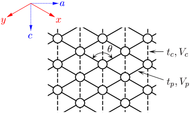
Figure 1: (Color online) Schematic representation of the anisotropic triangular-lattice Hubbard model. Each circle denotes an ET molecule.

The Hamiltonian of the extended Hubbard model defined on the anisotropic triangular lattice is given by

$$H= - \sum_{\left\langle ij\right\rangle\sigma}t_{ij}(c_{i\sigma}^{\dagger}c_{j\sigma}+{\rm H.c.})$$ (1)

$$+ U\sum_{i}n_{i\uparrow}n_{i\downarrow}+\sum_{\left\langle ij\right\rangle}V_{ij}n_{i}n_{j}$$

where $c_{i\sigma}^{\dagger}$ ($c_{i\sigma}$) is the creation (annihilation) operator of a hole with spin $\sigma$ at site $i$, $n_{i\sigma}=c_{i\sigma}^{\dagger}c_{i\sigma}$ is the number operator, and $n_{i}=n_{i\uparrow}+n_{i\downarrow}$. The sum $\left\langle ij\right\rangle$ runs over nearest-neighbor pairs. $t_{ij}$ and $V_{ij}$ are hopping integral and intersite Coulomb repulsion between sites $i$ and $j$; here we retain two kinds of nearest-neighbor hopping integrals (repulsions) $t_{p}$ ($V_{p}$) and $t_{c}$ ($V_{c}$) as shown in Fig. 1. $U$ is the onsite Coulomb repulsion. We restrict ourselves to the case at quarter filling; i.e., $\left\langle n_{i}\right\rangle=0.5$ where $\left\langle\cdots\right\rangle$ denotes the ground-state expectation value. In this paper, we consider the case of $U/t_{p}=10$ and $t_{c}/t_{p}=0$ as a typical set of parameter for X=CsCo(SCN)₄. Mori98 Hereafter, we take $t_{p}=1$ as the unit of energy.

II.2 Physical quantities

We employ two kinds of numerical methods, i.e., the DMRG and Lanczos methods. Either of these methods is chosen for the calculation of each physical quantity. The details are explained in the following.

II.2.1 Static quantities

We are interested in the CO phenomena in the subject materials, so that it is useful, first of all, to make the ground-state phase diagram associated with the charge degrees of freedom. To this end, we calculate the hole density $\left\langle n_{i}\right\rangle$ and double occupancy $\left\langle d_{i}\right\rangle$ ($d_{i}=n_{i\uparrow}n_{i\downarrow}$) for all sites $i$ to investigate the charge distribution. A large size system is required for reproducing all possible CO patterns and for an accurate estimation of these quantities. We thus study a finite-size cluster of $L_{a}=8$ and $L_{c}=6$ using the DMRG method. The periodic boundary conditions (PBC) are applied for the $c$-direction, whereas the open-end boundary conditions (OBC) are applied for the $a$-direction. This choice of the boundary conditions enables us to detect the CO state clearly (see Sec.III A). We keep up to $m\simeq 1400$ density-matrix eigenstates in the DMRG procedure and thus the maximum truncation error, i.e., the discarded weight, is less than $1\times 10^{-4}$. In this way, the maximum error in the ground-state energy is estimated to be $\Delta E_{0}/N\sim 10^{-2}$ for the most inaccurate case $V_{p}=V_{c}=0$. Based on the results of the hole density and double occupancy, we determine the ground-state phase diagram on the parameter space $(V_{p},V_{c})$.

II.2.2 Dynamical density-density correlation

Next, we consider the dynamical density-density correlation function defined as

$$N({\bf q},\omega)=\sum_{\nu}|\langle\psi^{N_{h}}_{\nu}|\hat{n}_{\bf q}|\psi^{N_{h}}_{0}\rangle|^{2}\delta(\omega-E_{\nu}+E_{0})$$ (2)

in order to study the low-energy charge excitations. Here, $|\psi^{N_{h}}_{\nu}\rangle$ and $E^{N_{h}}_{\nu}$ are the $\nu$-th eingenstate and eigenenergy of the system with $N_{h}$ holes ($\nu=0$ corresponds to the ground state). Since the exact definition of the momentum-dependent operators with the OBC is quite difficult, we choose the PBC for a quantitative estimation of the spectrum; we therefore use the PBC for both the $x$- and $y$-directions (or the $a$- and $c$-directions). With this PBC, the density operators $\hat{n}_{\bf q}$ can be precisely defined by

$$\hat{n}_{\bf q}=\frac{1}{\sqrt{N}}\sum_{i}e^{i{\bf q}\cdot{\bf r}_{i}}n_{i}$$ (3)

where $N$ is the number of lattice sites $L_{x}\times L_{y}$ (or $L_{a}\times L_{c}$) and ${\bf r}_{i}$ is the position of site $i$. However, in this case, it is quite difficult to carry out sufficiently accurate calculations with the DMRG method, so that we here use the Lanczos method on small clusters with 16 ($L_{x}=4$, $L_{y}=4$) and 18 ($L_{a}=6$, $L_{c}=3$) sites. Consequently, the system size is restricted but the result is numerically exact.

II.2.3 Single-particle excitation spectrum

Of interest are also the evolution of the fundamental excitations in the systems with strongly frustrated correlations. To see this, we calculate the single-particle excitation spectrum, which is obtained as

$$A({\bf q},\omega)=A^{-}({\bf q},-\omega)+A^{+}({\bf q},\omega)$$ (4)

with the photoemission (PES) spectrum

$$A^{-}({\bf q},\omega)=\sum_{\nu\sigma}|\langle\psi^{N_{h}-1}_{\nu}|\hat{c}_{{\bf q}\sigma}|\psi^{N_{h}}_{0}\rangle|^{2}\delta(\omega-E^{N_{h}-1}_{\nu}+E^{N_{h}}_{0})$$ (5)

and inverse photoemission (IPES) spectrum

$$A^{+}({\bf q},\omega)=\sum_{\nu\sigma}|\langle\psi^{N_{h}+1}_{\nu}|\hat{c}^{\dagger}_{{\bf q}\sigma}|\psi^{N_{h}}_{0}\rangle|^{2}\delta(\omega-E^{N_{h}+1}_{\nu}+E^{N_{h}}_{0})$$ (6)

where $\hat{c}^{\dagger}_{{\bf q}\sigma}$ ($\hat{c}_{{\bf q}\sigma}$) is the Fourier transform of the creation (annihilation) operator $\hat{c}^{\dagger}_{i\sigma}$ ($\hat{c}_{i\sigma}$). For the same reason as the calculation of the dynamical density-density correlation function, we employ the Lanczos method with the PBC where the operator is defined by

$$\hat{c}_{{\bf q}\sigma}=\frac{1}{\sqrt{N}}\sum_{i}e^{i{\bf q}\cdot{\bf r}_{i}}\hat{c}_{i\sigma}.$$ (7)

The calculation is carried out with a 18-site ($L_{a}=6$, $L_{c}=3$) cluster.

II.2.4 Optical conductivity

Finally, for more elaborate study on the behavior of the charge degrees of freedom and direct comparison with experiments, we calculate the optical conductivity defined by

$$\sigma_{\alpha}(\omega)=\frac{\pi}{N}\sum_{\nu}\omega|\langle\psi_{\nu}|\hat{D}_{\alpha}|\psi_{0}\rangle|^{2}\delta(\omega-E_{\nu}+E_{0}),$$ (8)

with a component of the dipole operator

$$\hat{D}_{\alpha}=-e\sum_{i}{\bf r}_{i}\cdot{\bf v}_{\alpha}(n_{i}-\frac{1}{2}),$$ (9)

where ${\bf v}_{\alpha}$ is a unit vector parallel to the $\alpha$-direction. It is known that the OBC is more feasible for calculation of the optical conductivity spectra because finite-size effects have much smaller influence on the results in comparison with a case using the PBC. Moskvin03 Hence, we apply the OBC for both the $a$- and $c$-directions and study a finite-size cluster $L_{a}=8$, $L_{c}=6$ with the dynamical DMRG (DDMRG) method. The DDMRG method is an extension of the standard DMRG method for the calculation of dynamical properties. In the DDMRG calculation, a required CPU time increases rapidly with the number of the density-matrix eigenstates $m$, so that we try to keep it as few as possible. Because the DMRG approach is based on a variational principle, we have to prepare a ‘good trial function’ of the ground state with the density-matrix eigenstates as much as possible. We therefore keep $m\sim 600$ to obtain the true ground state in the first five DDMRG sweeps and keep $m\sim 350$ to calculate the spectrum of the system. As a result, the maximum truncation error, i.e., the discarded weight, is about $1\times 10^{-3}$, while the maximum error in the ground-state is about $\Delta E_{0}/N\sim 2\times 10^{-2}$.

III Results

III.1 Ground-state phase diagram

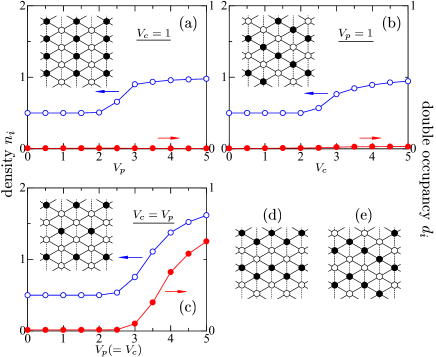
Figure 2: (Color online) Hole density $\left\langle n_{i}\right\rangle$ and double occupancy $\left\langle d_{i}\right\rangle$ at the hole-rich sites for (a) $V_{p}=1$, (b) $V_{c}=1$, and (c) $V_{p}=V_{c}$. The inset shows the schematic representation of (a) the diagonal stripe, (b) vertical stripe, and (c) three-fold CO patterns. The solid circle denotes a site where the hole predominantly resides. The other configurations are also shown: (d) horizontal and (e) an example of randomly aligned CO patterns.

So far, it has been suggested that the system defined by Eq.(1) has three types of CO phases, depending on the values of the intersite Coulomb repulsions. The CO patterns for each phase are shown in the inset of Fig. 2: (a) vertical stripe for $V_{c}\ll V_{p}$, (b) diagonal stripe for $V_{c}\gg V_{p}$, and (c) three-fold alignment for $V_{c}\sim V_{p}\gg t_{p}$. Other likely patterns are also shown: (d) horizontal and (e) randomly aligned stripes, which are not realized in the ground state. A random alignment CO pattern is formed with any combination of alternately-occupied chains parallel to the $c$-axis. Hence, the diagonal CO pattern is a special case of the random alignment ones.

First of all, we note that the CO is observed as a state with a broken translational symmetry in our calculations: actually, there are two or more degenerate ground states and one of the degenerate states is picked out as the ground state by an initial condition of the DMRG calculation as we here apply the OBC along the $x$-direction. Thus, a CO state includes more than two kinds of sites with different hole densities, i.e., hole-rich and hole-poor sites. In Fig. 2, we show DMRG results of the hole density $\left\langle n_{i\in{\rm rich}}\right\rangle$ and double occupancy $\left\langle d_{i\in{\rm rich}}\right\rangle$ at the hole-rich sites $i\in{\rm rich}$ for (a) $V_{c}=1$, (b) $V_{p}=1$, and (c) $V_{p}=V_{c}$. When both $V_{p}$ and $V_{c}$ are small, the analysis shows that the hole density is uniform over the system, i.e., $\left\langle n_{i}\right\rangle=0.5$ for all sites $i$, and the system is in the metallic state. As $V_{p}$ and/or $V_{c}$ increase, the charge fluctuations toward the CO states are enhanced and we find that $\left\langle n_{i\in{\rm rich}}\right\rangle$ starts to increase at the CO phase boundary. In the CO phase, the charge fluctuations are weakened again as the CO state is stabilized, where $\left\langle n_{i\in{\rm rich}}\right\rangle$ approaches a value in the atomic limit $t_{p}\to 0$.

Let us now evaluate the phase boundaries between the metallic and CO phases. When we increase $V_{p}$ from zero with fixing $V_{c}=1$ [see Fig. 2(a)], $\left\langle n_{i\in{\rm rich}}\right\rangle$ begins to increase around $V_{p}=2.5$; accordingly, a critical strength of the vertical CO state is obtained as $(V_{p}^{\rm c},V_{c}^{\rm c})\sim(2.5,1)$. At $V_{p}>V_{p}^{\rm c}$, $\left\langle n_{i\in{\rm rich}}\right\rangle$ increases rapidly to unity but the double occupancy remains almost zero. This means that (nearly) half-filled chains are alternated with (nearly) empty chains and the charge fluctuations are totally suppressed in the entire region of vertical CO phase. In analogy with the case of the vertical CO state, we can estimate a critical strength of the diagonal CO state as $(V_{p}^{\rm c},V_{c}^{\rm c})\sim(1,2.75)$ [see Fig. 2(b)]. We should however note that $\left\langle n_{i\in{\rm Rich}}\right\rangle$ seems to approach unity more slowly than that in the vertical CO phase. This implies that the charge fluctuations in the diagonal CO state are rather stronger than those in the vertical CO state. The reason of this strong charge fluctuation in the diagonal CO phase is the existence of nearly energetically degenerate states, i.e., the horizontal and an infinite number of the randomly aligned CO patterns, which are shown in Fig. 2(d) and (e), respectively. This situation has also been confirmed by the mean-field approximation, Kaneko06 variational Monte Carlo (VMC) method, Watanabe06 and strong-coupling study of the spinless model. Hotta06 The energies of those CO patterns including the diagonal one are exactly equal to each other in the atomic limit $t_{p}\to 0$.

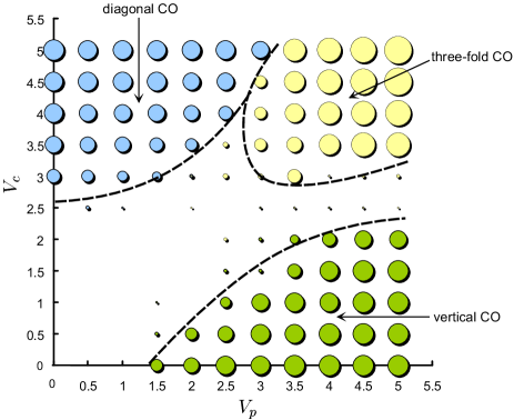
Figure 3: (Color online) Ground-state phase diagram of the extended Hubbard model defined on the anisotropic triangular lattice. We assume the values $t_{\rm c}=0$ and $U=10$. The result is obtained from the DMRG calculations for the charge distributions with a broken translational symmetry. The diameter of the circles is taken to be proportional to the hole density at the hole-rich sites.

As for the three-fold CO phase, the situation is somewhat different from the other CO phases. If a relation $V_{c}=V_{p}$ is kept, the three-fold CO instability begins to appear around a critical point $(V_{p}^{\rm c},V_{c}^{\rm c})\sim(3,3)$ [see Fig. 2(c)]. Above the critical point, we find the rapid increase of not only the hole density but also the double occupancy at the hole-rich sites. This implies that the competition between the effects of $U$ and $V$’s is essential for the presence of the three-fold CO phase. We also note that the three-fold CO state is metallic in the sense that the Drude weight is nonzero. Shingai The presence of metallic CO phase has previously been suggested for the extended square-lattice Hubbard models; simply, the pocket-like small Fermi surface appears by doping the long-range CO phases with holes or electrons without destroying the long-range CO. Ohta94 Note that the ground state has both the onsite hole-pairing and CO, which may be essentially the same as the coexistence of the s-wave superconducting and CO states in the two-dimensional negative-$U$ Hubbard model. Scalettar89

In Fig. 3, we determine the ground-state phase diagram from the results of the hole density, where the phase boundaries are drawn with dashed curves. We can make it certain that the three substantial CO phases are distinguished from a metallic phase with uniform charge distribution. This phase diagram is basically consistent with that from the VMC calculation. Watanabe06 The main difference is that a metallic region is sandwiched between the vertical and three-fold CO phases in our results. On the other hand, the diagonal and three-fold CO phases are contiguous, in agreement with the VMC result. The appearance of the metallic region in-between may be explained as follows. The diagonal and three-fold CO phases may be contiguous because the transition can be derived by the flow of charges only via the nearest-neighbor hopping integrals $t_{p}$ (see Fig. 4), whereas a drastic charge redistribution is required in the transition from the vertical CO pattern to the three-fold CO pattern and therefore the ground state needs to go through the metallic one. We may also suggest that this ‘charge-flowing’ transition between the diagonal and three-fold CO phases occurs in the presence of the three-fold (diagonal) charge fluctuations in the diagonal (three-fold) CO phase as is evident in the calculated dynamical density-density correlation functions (see the following subsection). We also note that the three-fold CO phase is shrunk with increasing $U$.

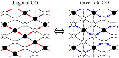
Figure 4: (Color online) Transition between diagonal and three-fold CO states. The solid circle denotes a site where hole predominantly resides. The arrows denote the flow of charges toward the other CO state.

III.2 Dynamical density-density correlation

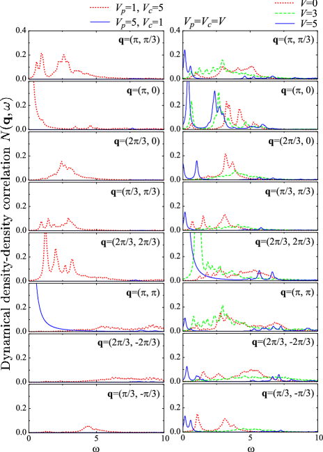
Figure 5: (Color online) Charge excitation spectra calculated for the 18-site cluster with the Lanczos exact-diagonalization method. Only the results of $(\pi,0)$ are obtained for the 16-site cluster. Spectra at $(V_{p},V_{c})=(1,5)$, $(5,1)$ [left panel], $(0,0)$, $(3,3)$, and $(5,5)$ [right panel] are shown.

The dynamical density-density correlation functions calculated by the Lanczos method for several sets of $V_{p}$ and $V_{c}$ values are shown in Fig. 5. Each parameter set corresponds to a different phase as follows: $(V_{p},V_{c})=(1,5)$ to the diagonal CO phase, $(5,1)$ to the vertical CO phase, $(5,5)$ to the three-fold CO phase, and $(0,0)$ to the uniform metallic phase. In addition, we plot the results for $(V_{p},V_{c})=(3,3)$, where the system is in the non-CO metallic phase but with strong three-fold CO fluctuations. When $(V_{p},V_{c})=(0,0)$, the model (1) is equivalent to the square-lattice Hubbard model at quarter filling and no particular modes of charge fluctuations are developed; we therefore find the broad spectral features for all the momenta, which come basically from the particle-hole transition in the corresponding noninteracting system. With increasing the intersite interactions, however, the broad features change to the low-energy sharp peaks, indicating that the excitations turn to be collective-mode like.

Generally, the enhancement of low-lying peak at a particular momentum must be expected for the CO instability. When the system is unstable to the vertical [diagonal] CO phase, the particular momentum is located at ${\bf q}=(\pi,\pi)$ [${\bf q}=(\pi,0)$]. Looking at the spectra for $(V_{p},V_{c})=(5,1)$, a sharp peak appears around $\omega=0$ at ${\bf q}=(\pi,\pi)$ and there are nearly no peaks at the other momenta. This means that the system is unstable to the vertical CO state with (almost) complete charge disproportionation. This result is consistent with the results of the hole density given in Sec. III A. On the other hand, in the spectra at $(V_{p},V_{c})=(1,5)$, we see not only a low-energy peak at $(\pi,0)$ but also relatively high-energy peaks at the other momenta; most of the high-energy peaks concentrate at momenta with $q_{x}q_{y}>0$ and few peaks appear at momenta with $q_{x}q_{y}<0$. By the axes rotation, we find the charge fluctuations mostly occur along the $c$-axis, which are associated with the nearly degenerate states, i.e., horizontal and randomly aligned CO phases. It is moreover striking that the intensity around ${\bf q}=(2\pi/3,2\pi/3)$ is significantly large, which means that the three-fold charge fluctuations are rather strong although the system is in the diagonal CO phase.

Let us now discuss the spectral features for the three-fold CO metallic state, of which the particular momentum is located at ${\bf q}=(2\pi/3,2\pi/3)$. The charge excitation spectra in the CO metallic state are currently not well understood, so that a good opportunity for studying them may be offered here. We thus investigate a process of gradual change in the spectra with increasing the intersite Coulomb interactions $V$’s. Since the three-fold CO phase lies around $V_{p}\sim V_{c}>3$, we increase $V_{p}$ ($V_{c}$) from $0$ to $5$ with keeping a condition $V_{p}=V_{c}$. The spectra for $(V_{p},V_{c})=(0,0)$ have the broad spectral features for all the momenta as mentioned above and these features basically remain unchanged as far as $V_{p}$ and $V_{c}$ are less than $\sim 2$. Only around $(V_{p},V_{c})=(3,3)$, we can recognize the changes clearly in the calculated spectra: the low-energy spectrum at ${\bf q}=(2\pi/3,2\pi/3)$ is particularly enhanced as anticipated, but those at ${\bf q}=(\pi,0)$ and ${\bf q}=(\pi,\pi)$ are also enlarged, while the spectral weights for the other momenta are strongly suppressed. We understand that these changes suggest that the three types of CO instability are simultaneously developed and that, considering that the energies of the lowest-lying excitations for the three momenta are nearly equal, the charge fluctuations for the three CO patterns are strongly competing.

After increasing the intersite Coulomb interactions to $(V_{p},V_{c})=(5,5)$, even greater changes are seen in the spectral features. At ${\bf q}=(2\pi/3,2\pi/3)$, we find the enhancement of a sharp peak around $\omega=0$, which indicates the strong charge fluctuations of the three-fold periodicity and is consistent with the results of the hole density. It is particularly worth noting that the low-energy spectral intensities at $(\pi,0)$ is continuously enhanced [and those at $(\pi,\pi)$ are suppressed].

Let us discuss some experimental situations here. We may point out first that the wave vectors ${\bf q}_{1}$ and ${\bf q}_{2}$ of the two diffuse peaks observed experimentally Nogami99 ; Watanabe99 in the CO phase of $\theta$-(ET)$MM^{\prime}$(SCN)₄ [$M=$Cs, $M=$Co or Zn] should be equivalent to our momenta $(\pi,0)$ and $(2\pi/3,2\pi/3)$, respectively. We may therefore suggest that the appearance of the two enhanced peaks in our calculations correspond to the coexistence of the two different charge fluctuations. Note that these enhanced peaks are already obtained for more realistic parameter values $(V_{p},V_{c})=(3,3)$ in our calculations. It is also striking that the low-energy peaks appear in the entire Brillouin zone and the charge fluctuations are induced in all the momentum transfers. This situation is quite different from those for the diagonal and vertical CO stripes where the low-energy peak appears only at the particular momenta.

III.3 Single-particle excitation spectrum

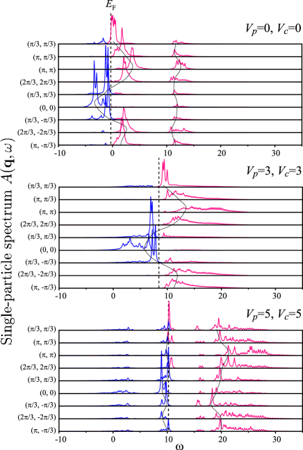
Figure 6: (Color online) Single-particle excitation spectra calculated for the 18-site cluster with the Lanczos exact-diagonalization method. The dashed lines denote the Fermi levels and the thin lines mark the dispersion of bands.

In the diagonal and vertical CO phases, we just find the insulating band structures reflecting the CO states in our calculations; namely, the PES and IPES peaks are separated by the charge gap and the Fermi level lies between the two spectra. We thus focus on the spectral features in the three-fold CO phases here. In Fig. 6, we show the single-particle excitation spectra calculated with the Lanczos method for $(V_{p},V_{c})=(0,0)$, $(3,3)$, and $(5,5)$. At $(V_{p},V_{c})=(0,0)$, we can clearly see the spectral weight separated into two bands due to the onsite Coulomb interaction, i.e., lower Hubbard band (LHB) and upper Hubbard band (UHB) with the distance $\sim 10$ ($=U$). The LHB, which corresponds to the conduction band, can be approximately expressed by the dispersion of noninteracting holes,

$$\varepsilon_{\bf q}=-2t_{p}\cos q_{x}-2t_{p}\cos q_{y}.$$ (10)

On the other hand, the UHB has relatively small spectral weight and narrow band width, which are general features in the strong-coupling regime. At $(V_{p},V_{c})=(3,3)$, the shape of conduction band remains almost unchanged from that at $(V_{p},V_{c})=(0,0)$. However, we can see that an overlap between the LHB and UHB occurs due to the competition between the onsite and nearest-neighbor Coulomb interactions. As a result, the band structure is seen to be reduced to a single dispersion line. The interaction between holes is effectively weakened (or vanished) by the frustration of the Coulomb interactions, so that the dispersion relation looks as if it were for the single-orbital model or the noninteracting case.

Surprisingly, the spectral features are drastically changed at $(V_{p},V_{c})=(5,5)$. The spectral weight appears to be separated to form several bands again. It is particularly worth noting that the width of conduction band is much narrower than that at $(V_{p},V_{c})=(3,3)$. In the three-fold CO phase, the holes can conduct only through the hole-rich sites but the hole-rich sites are not connected by direct hopping integrals; in other words, the carriers form a small Fermi surface. Ohta94 Thus, the conduction band is centered at $\omega\sim 10(=U)$ and the band width should be very narrow. It may be related to the appearance of low-energy peaks in the entire Brillouin zone observed in the dynamical density-density correlation function as discussed above. Let us then consider the peaks in the higher-energy range, $\omega\gtrsim 15$. These peaks are essentially formed in connection with the empty (hole-poor) sites. An empty site is surrounded by three hole-rich sites and a hole-rich site is occupied by one or two holes. When a hole is added on an empty site, the excitation energy is $\omega\sim 2V_{p}+V_{c}=15$ if the surrounding three hole-rich sites are singly occupied and it is $\omega\sim 4V_{p}+2V_{c}=30$ if the surrounding three hole-rich sites are doubly occupied. This is the reason why there are continuum weights from $\omega\sim 15$ to $30$ in the spectra for all the momenta. In addition, we can find the dispersion with bandwidth $\sim 4$ around $\omega=20$. This dispersion is formed from a empty zigzag chain along the $a$-axis, which is nearly separated from each other by the hole-rich sites.

III.4 Optical conductivity

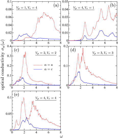
Figure 7: (Color online) Optical conductivity spectra calculated with the DDMRG method. $\alpha(=a,c)$ is the direction of the electric field defined in Fig. 1.

The optical conductivity spectra calculated by the DMRG method for several sets of $V_{p}$ and $V_{c}$ are shown in Fig. 7. For all cases, the spectral intensity for the $a$-direction seems to be a few times larger than that for the $c$-direction, which just reflects the difference between the interatomic distances $d_{a}:d_{c}=\sqrt{3}:1$ in the $a$ and $c$ directions. This leads to the intensity ratio $I_{a}:I_{c}=3:1$.

The most easily comprehensible result should be the ones in the vertical CO phase, i.e., $(V_{p},V_{c})=(4,1)$ [see Fig. 7(b)]. The shapes of spectra for the $a$- and $c$-directions are essentially the same, although the intensities are different as mentioned above. For both of the spectra, the lowest excitation appears around $\omega\sim 2.5$, which corresponds to the optical (insulating) gap, and the other excitations lie in much higher frequencies, $\omega\gtrsim 4$. Also, the total weight of the spectrum is smaller than that in the other CO phases. These results are consistent with the fact that the vertical CO state is rather solid and the charge fluctuations are quite small. The optical gap in the vertical CO phase may be estimated as $\sim 3V_{p}-2V_{c}-W$ with the bare bandwidth $W=8$.

Let us then turn to the diagonal CO phase, i.e., $(V_{p},V_{c})=(1,4)$ [see Fig. 7(a)]. We find that the result for the $a$-direction is apparently different from that for the $c$-direction. The spectrum for the $a$-direction consists of the first-excitation peak at $\omega\sim 2.2$ and high-energy broad features, which is similar to that in the vertical CO phase. This result reflects the solid CO and weak charge fluctuations along the $a$-direction, as shown in the dynamical density-density correlation functions. On the other hand, most of the spectral features for the $c$-direction appear in the lower-energy range. The optical gap is of the order of $\sim 0.5$, which is much smaller than that of the vertical CO phase. This is so because the diagonal CO state can be rearranged to the randomly aligned (or horizontal) CO state with small excitation energy. Thus, the charge fluctuations along the $c$-axis are much stronger than those along the $a$-axis. Since the energy difference between the diagonal CO phase and random alignment CO state is hardly changed even if $V_{c}$ increases, the low-energy structure is expected to be seen for any $V_{c}$ value.

Lastly, we discuss the spectral aspects in the metallic regime around the three-fold CO instability [see Fig. 7(c)-(e)]. With the OBC, the optical conductivity at $\omega=0$ is ruled out and the lowest-energy scale is limited to an order of $4W/L_{a}L_{b}\sim 0.67$. Fye91 Therefore, the Drude spectral weight appears around the minimum excitation energy. At $(V_{p},V_{c})=(2,2)$, the spectra for the $a$- and $c$-directions are quite similar. For each spectrum, small peak structure around $\omega\sim 0.7-0.8$ should correspond to the Drude peaks. The spectral weight exists continuously from the ‘Drude frequency’ to higher excitations and reaches the maximum around $\omega=2$, and very little spectral weight exists at higher-energy range, $\omega\gtrsim 3$. At $(V_{p},V_{c})=(3,3)$, we can find some tendencies to the three-fold CO state; in the spectrum along the $a$-axis the intensity around $\omega=2$ is about half of that at $(V_{p},V_{c})=(2,2)$ and the high-energy broad features are relatively large. A large peak around $\omega=2$ at $(V_{p},V_{c})=(2,2)$ splits into two peaks that indicate the appearance of individual excitations associated with the COs. The spectrum along the $a$-axis remains almost unchanged, except the Drude-like peak which becomes much smaller. At $(V_{p},V_{c})=(4,4)$, we can clearly see the characteristic features of the three-fold CO state: in the spectrum along the $a$-axis the weight is separated into the low-energy Drude-like peak at $\omega\sim 0.7-0.8$ and high-energy broad features. We can understand that the former comes from the small Fermi surface in the three-fold CO phase and the latter comes from the excitations due to the three-fold charge fluctuations. On the other hand, the weight of the Drude-like peak is nearly zero in the spectrum along the $c$-axis. This means that the CO is more solid along the $c$-axis than along the $a$-axis. We can explain this as follows: 3/2-filled chains are alternated with zigzag empty chains along the $c$-axis [see the inset of Fig. 2 (c)], whereas each chain along the $c$-axis is quarter filled, which means that the holes distribute uniformly along the $a$-axis. As mentioned above, the optical conductivity along the $a$- ($c$-) axis is concentrated in the lower-energy range when the three-fold (diagonal) charge fluctuations are enhanced. We suggest that these features in the optical conductivity spectra should give a good criterion to examine the CO patterns experimentally.

IV Conclusions

The extended Hubbard model at quarter filling defined on the anisotropic triangular lattice have been studied by the Lanczos exact-diagonalization and DMRG methods. We determine the ground-state phase diagram based on the results of the hole density and double occupancy. In the phase diagram, there exist three substantial CO phases (diagonal, vertical, and three-fold) and a metallic phase with uniform charge distribution. We find that the charge fluctuations (or instability to CO) with the three-fold periodicity appear for realistic parameters $V_{p}\sim V_{c}\sim 0.3U$.

We suggest that the transition between the diagonal and three-fold CO phases is derived by the flow of charges only via the nearest-neighbor hopping integrals, which may lead to the coexistence of the diagonal and three-fold charge fluctuations near the phase boundary. The coexistence features are also found in the density-density correlation functions; in the diagonal (three-fold) phase, not only the particular peak but also the low-energy peaks corresponding to the three-fold (diagonal) charge fluctuations are enhanced. In the vertical CO phase, only the low-energy peak at the particular momentum is visible and there is no charge fluctuations associated with the other CO states. Moreover, we find that there appear the low-energy collective-modes-like excitations in the entire Brillouin zone when the three-fold charge fluctuations are very strong. The wave numbers of the diagonal and three-fold charge fluctuations are equivalent to those of the two X-ray diffuse peaks ${\bf q}_{1}=(0,k,1/2)$ and ${\bf q}_{2}=(2/3,k,1/3)$ measured in $\theta$-(ET)Cs$M^{\prime}$(SCN)₄ with $M=$Co or Zn. If we could make the dihedral angle larger, the value of $V_{p}/V_{c}$ decreases and only the diagonal CO fluctuation remains. This is consistent with the fact that only a diffuse peak with wave number ${\bf q}_{1}$ is observed in the compounds with $M=$Tl and Rb which have a larger dihedral angle than those with $M=$Co or Zn do.

We also study the single-particle excitation spectrum to see the evolution of the fundamental low-lying excitations in the presence of strongly frustrated correlations. When the onsite and intersite Coulomb interactions compete ($V_{p}\sim V_{c}\sim U/3$), the interaction between holes is effectively diminished and the dispersion relation looks as if it is of the noninteracting case. When the two intersite Coulomb interactions compete ($V_{p}\sim V_{c}>U/3$), the carriers form very narrow conduction band with a small Fermi surface.

Furthermore, we examine the optical conductivity which reflects the characteristic features for each CO phase. In the vertical CO phase, the spectra for both the directions explicitly represent the insulating features and the optical gaps are large, estimated as $\sim 3V_{p}-2V_{c}-8$. In the diagonal CO phase, the spectrum for the $a$-direction is essentially the same as that in the vertical CO phase but that for the $c$-direction is located in the lower-energy range. This is so because the diagonal CO state can be rearranged to the randomly aligned (or horizontal) CO state with small excitation energy. In the three-fold CO phase, the spectra indicate the presence of the separated low-energy Drude-like peak and high-energy broad features, leading to the anomalous metallic states in the system. The optical conductivity along the $a$- ($c$-) axis is concentrated in the lower-energy range when the three-fold (diagonal) charge fluctuations. These spectral features may give a good criterion to examine the CO patterns experimentally. Finally, we make a comment on the difference in the experimental spectra between $MM^{\prime}=$CsZn and $MM^{\prime}=$RbZn. Because we find that an increase in $V_{p}/V_{c}$ makes the diagonal CO state unstable, it is the smallness of $t_{c}$ that is essential for the strong insulating features in the spectra of $MM^{\prime}=$CsZn.

We hope that our studies will help us understand the mechanism of charge fluctuations in the extended Hubbard model defined on the anisotropic triangular lattices and hence will offer useful suggestions to some aspects of the three-fold charge fluctuations observed in $\theta$-(ET)₂X.

- (1) Present address: Leibniz-Institut für Festkörper- und Werkstoffforschung Dresden, P.O. Box 270116, D-01171 Dresden, Germany
- (2) Y. Tokura and N. Nagaosa, Science 288, 462 (2000).
- (3) E. J. W. Verwey and P. W. Haayman, and F. C. Romeijn, J. Chem. Phys. 15, 181 (1947).
- (4) S. Mori, C. H. Chen, and S.-W. Cheong, Nature 392, 473 (1998).
- (5) J. M. Tranquada, B. J. Sternlieb, J. D. Axe, Y. Nakamura, and S. Uchida, Nature 375, 561 (1995).
- (6) M. Lang and J. Müller, The Physics of Superconductors - Vol.II, edited by K.-H. Bennemann and J. B. Ketterson (Springer, Berlin, 2003), p.453.
- (7) H. Mori, S. Tanaka, and T. Mori, Phys. Rev. B57, 12023 (1998);
- (8) H. Mori, T. Okano, S. Tanaka, M. Tamura, Y. Nishio, K. Kajita, and T. Mori, J. Phys. Soc. Jpn. 69, 1751 (2000).
- (9) H. Kobayashi, R. Kato, A. Kobayashi, Y. Nishio, K. Kajita, and W. Sasaki, Chem. Lett. 1986, 789 (1986); 1986 833 (1986).
- (10) K. Miyagawa, A. Kawamoto, and K. Kanoda, Phys. Rev. B62, R7679 (2000).
- (11) R. Chiba, H. Yamamoto, K. Hiraki, T. Takahashi and T. Nakamura, J. Phys. Chem. Solids 62, 389 (2001).
- (12) M. Watanabe, Y. Noda, Y. Nogami, and H. Mori, Synth. Met. 135-136, 665 (2003).
- (13) M. Watanabe, Y. Noda, Y. Nogami, and H. Mori, J. Phys. Soc. Jpn. 73, 116 (2004);74, 2011 (2005).
- (14) H. Seo, J. Phys. Soc. Jpn. 69, 805 (2000).
- (15) Y. Nogami, J.-P. Pouget, M. Watanabe, K. Oshima, H. Mori, S. Tanaka and T. Mori, Synth. Met. 103 1911 (1999).
- (16) M. Watanabe, Y. Nogami, K. Oshima, H. Mori, and S. Tanaka, J. Phys. Soc. Jpn. 68, 2654 (1999).
- (17) K. Inagaki, I. Terasaki, H. Mori, and T. Mori, J. Phys. Soc. Jpn. 73, 3364 (2004).
- (18) T. Nakamura, W. Minagawa, R. Kinami, and T. Takahashi, J. Phys. Soc. Jpn. 69, 504 (2000).
- (19) R. Chiba, K. Hiraki, T. Takahashi, H. M. Yamamoto, and T. Nakamura, Synth. Met. 133-134, 305 (2003).
- (20) F. Sawano, I. Terasaki, H. Mori, T. Mori, M. Watanabe, N. Ikeda, Y. Nogami, and Y. Noda, Nature 437, 522 (2005).
- (21) Y. Takahide, T. Konoike, K. Enomoto, M. Nishimura, T. Terashima, S. Uji, and H. M. Yamamoto, Phys. Rev. Lett. 96, 136602 (2006).
- (22) N. L. Wang, T. Feng, Z. J. Chen, and H. Mori, Synth. Met. 135-136, 701 (2003).
- (23) K. Suzuki, K. Yamamoto, K. Yakushi, and A. Kawamoto, J. Phys. Soc. Jpn. 74, 2631 (2005).
- (24) M. Kaneko and M. Ogata, J. Phys. Soc. Jpn. 75, 014710 (2006).
- (25) H. Watanabe and M. Ogata, J. Phys. Soc. Jpn. 75, 063702 (2006).
- (26) C. Hotta and N. Furukawa, Phys. Rev. B74 193107 (2006); C. Hotta, N. Furukawa, A. Nakagawa, and K. Kubo, J. Phys. Soc. Jpn. 75, 123704 (2006).
- (27) K. Kuroki, J. Phys. Soc. Jpn. 75, 114716 (2006).
- (28) H. Seo, K. Tsutsui, M. Ogata, and J. Merino, J. Phys. Soc. Jpn. 75, 114707 (2006).
- (29) M. Udagawa and Y. Motome, Phys. Rev. Lett. 98, 206405 (2007).
- (30) M. Shingai, S. Nishimoto, and Y. Ohta, unpublished.
- (31) Y. Ohta, K. Tsutsui, W. Koshibae, and S. Maekawa, Phys. Rev. B50, 13594 (1994).
- (32) R. T. Scalettar, E. Y. Loh, J. E. Gubernatis, A. Moreo, S. R. White, D.J. Scalapino, R. L. Sugar, and E. Dagotto, Phys. Rev. Lett. 62, 1407 (1989); A. Moreo and D. J. Scalapino, Phys. Rev. Lett. 66, 946 (1991).
- (33) A. S. Moskvin, J. Málek, M. Knupfer, R. Neudert, J. Fink, R. Hayn, S.-L. Drechsler, N. Motoyama, H. Eisaki, and S. Uchida, Phys. Rev. Lett. 91, 037001 (2003).
- (34) R. M. Fye, M. J. Martins, D. J. Scalapino, J. Wagner, and W. Hanke, Phys. Rev. B44, 6909 (1991)