CERN-PH-TH/2008-039

SISSA 10/2008/EP

Metastable vacua and geometric deformations

Antonio Amariti^a, Davide Forcella^b, Luciano Girardello^a, Alberto Mariotti^a,c

^a Dipartimento di Fisica, Università di Milano Bicocca

and

INFN, Sezione di Milano-Bicocca,

piazza della Scienza 3, I-20126 Milano, Italy
^b International School for Advanced Studies (SISSA/ISAS)

and

INFN-Sezione di Trieste,

via Beirut 2, I-34014, Trieste, Italy

^b PH-TH Division, CERN CH-1211 Geneva 23, Switzerland

^c Service de Physique Theorique, SPhT

Orme des Merisiers, CEA/Saclay

91191 Gif-sur-Yvette Cedex, FRANCE

^c LPTHE, Universites Paris VI, Jussieu

F-75252 Paris, FRANCE

We study the geometric interpretation of metastable vacua for systems of D3 branes at non isolated toric deformable singularities. Using the $L^{aba}$ examples, we investigate the relations between the field theoretic susy breaking and restoration and the complex deformations of the CY singularities.

March 10, 2024

Introduction

The ISS mechanism [1], based on long living metastable vacua, greatly increases the class of gauge theories with chiral matter and dynamically broken supersymmetry. Much work has indeed followed, in different directions [2].

It has prompted a search for a string approach: either within the gauge/gravity correspondence or toward a more direct string origin or interpretation [3]-[14]. These remain open problems and only partial results are at hand.

Recently, some steps have emerged for the grounding of a geometrical interpretation of the features of metastability in simple quiver gauge theories on $D$-branes near a singularity inside a CY manifold [15, 16]. The aim is to phrase the metastable $F$-type susy breaking in a general geometrical language. A key point is that the non perturbative dynamics behind the existence of metastable vacua corresponds to deformations of a theory with unbroken suspersymmetry [15]. The deformations regard the superpotential: in the $D$-brane setting of IIB string theory they are mapped into complex deformations in the local geometry.

In this paper we develop this approach further. We study systems of branes at toric conical Calabi-Yau singularities of a special type, i.e. deformable singularities, in the sense of Altman’s deformations [17], that are not isolated. These form a large subfamily of toric singularities and consist of a cone with a singularity at the tip and some set of lines of $\mathbb{C}^{2}/\mathbb{Z}_{n}$ singularities passing through it. Different combinations of fractional branes at these singularities give rise to different IR behaviors of the gauge theory: $\mathcal{N}=2$ dynamics, confinement, runaway supersymmetry breaking [18], and long living metastable vacua, as recently pointed out in [15]. Some of the different IR dynamics can be geometrically understood as motion in the moduli space of the CY singularities.

Our discussion is mainly focused on metastability in the quiver gauge theories living on deformed $L^{aba}$ singularities. Such theories correspond to an infinite class of non isolated toric singularities, with a known metric. Beyond their role in model building and in the gauge/gravity duality, they form a fitting laboratory for the investigation of the field theory/geometry correspondence. In the analysis of general $L^{aba}$ quivers we show that we can always extract subclasses where metastable vacua exist. The features of broken and restored supersymmetry find a systematic geometric counterpart in terms of appropriate deformations of the geometry of the unbroken susy phase.

The plan of the paper is as follows. In section 1 we review the case of the Suspended Pinch Point ($SPP$) singularity, its associated field theory and the relation between their corresponding deformations. This simple case will be the guideline for the whole paper. In section 2 we introduce the family of $L^{aba}$ singularities and the corresponding quiver gauge theories. We then analyze the metastable vacua in the $L^{aba}$ gauge theories with $b\neq a$ in section 3, and the $L^{aaa}$ gauge theories in section 4. In all these cases we show that some deformation of the geometry leads to metastability and some other deformation restores supersymmetry. Metastability turns out to be a quite generic phenomenon in these deformed toric theories. Finally, in section 5 we try to extend this analysis to more complicated singularities. Since we shall use some elements of toric geometry we present in Appendix A a lightening review of a few aspects and instructions for drawing out information of interest in our investigation. In the Appendix B we review the ISS model and discuss the issue of gauging flavour. In the Appendix C we outline the technique introduced in [16] for the computation of the superpotential from the geometry. In the Appendix D we give details on the non supersymmetric vacua analyzed in the paper. In the Appendix E we discuss the problem of UV completion in a clarifying example.

1 Complex deformations and metastability: the SPP example

The SPP gauge theory [19] is obtained as the near horizon limit of a stack of D3 branes on the tip of the conical singularity

$$xy^{2}=wz\,.$$ (1)

The holomorphic equation defining the singularity can be encoded in a graph called the toric diagram (see the Appendix A). In the paper we will use these diagrams to give an intuitive visual picture of the singularities.
The field theory has $U(N_{1})\times U(N_{2})\times U(N_{3})$ gauge groups and chiral superfields that transform in the adjoint and bifundamental representations of the various gauge group factors. The fields $X_{ii}$ are in the adjoint of the i-th gauge group and the fields $q_{ij}$ transform in the fundamental representation of the $U(N_{i})$ gauge group and in the anti-fundamental representation of the $U(N_{j})$ gauge group. The symmetries and the matter content of a gauge theory related to branes at singularities can be encoded in a graph called the quiver diagram. The toric diagram and the quiver of the $SPP$ singularity are shown in Figure 1.

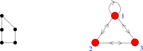
Figure 1: The toric diagram and the quiver of the $SPP$ singularity

Its superpotential is

$$W=X_{11}(q_{13}q_{31}-q_{12}q_{21})+q_{21}q_{12}q_{23}q_{32}-q_{32}q_{23}q_{31}q_{13}\,.$$ (2)

Taking into account the F-term equations for (2) we can choose

$$x=X_{11}=q_{23}q_{32}\hbox{ , }y=q_{12}q_{21}=q_{13}q_{31}\hbox{ , }w=q_{13}q_{32}q_{21}\hbox{ , }z=q_{12}q_{23}q_{31}$$ (3)

as generators of the mesonic chiral ring. The set of algebraic relations among these fields reproduces the geometric singularity (1). The presence of an adjoint chiral field is a signal for the presence of a non isolated singularity. In fact, giving a vev to $X_{11}$ corresponds to motion in the geometry along the $x$ direction, which is a line of non isolated $\mathbb{C}^{2}/\mathbb{Z}_{2}$ singularities: $y^{2}=wz$. This line of singularities can be deformed to a smooth space

$$xy^{2}=wz\rightarrow xy(y-\xi)=wz\,.$$ (4)

Moreover the conical singularity (1) has a complex deformation in which the tip of the cone is substituted by a three sphere $S^{3}$. In this case the SPP geometry is deformed as

$$xy^{2}-y\epsilon-wz=0\,.$$ (5)

This is the same process as the conifold transition in the KS solution [20].

Using toric geometry it is possible to visualize these two processes. First of all draw the toric diagram of the singularity.

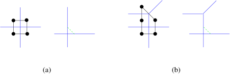
Figure 2: Toric diagram, dual diagram and complex deformation for (a) the conifold case $xy-wz=0\rightarrow xy-wz-\epsilon=0$; (b) the SPP case $xy^{2}-wz=0\rightarrow xy^{2}-y\epsilon-wz=0$. The broken line represents the $S^{3}$ due to the fluxes. The volume of $S^{3}$ is parameterized by $\epsilon$.

Then, if the dual graph has some parallel lines, this implies that there exist non isolated $\mathbb{C}^{2}/\mathbb{Z}_{k}$ lines of singularities (depending on the number of parallel lines). These singularities can be deformed by inserting two spheres $S^{2}$ parameterized by a set of complex $\xi_{i}$ parameters. If the dual diagram admits splits in equilibrium (the edges of every sub-diagrams sum to zero), there exist deformations of the singularities on the tip of the cone. These deformations are obtained by inserting three spheres $S^{3}$, parameterized by some set of complex $\epsilon_{j}$ parameters (see Figure 2).

In this paper we argue that metastable supersymmetry breaking is geometrically realized by moving in the space of complex deformations. The motion in the $\xi$-parameter space breaks supersymmetry (in a metastable vacuum) while moving in the $\epsilon$-parameter space restores the supersymmetry. We will provide several examples and show that this is a general phenomenon in an infinite class of quiver gauge theories.

We now review the possible IR behavior of the SPP gauge theory and their geometric interpretation. The SPP gauge theory has two kinds of fractional branes, because of the non anomalous distribution of ranks for the gauge group factors: $(1,0,0)$ and $(0,1,0)$. The different combinations of these set of branes and the possible geometric deformations of the singularity characterize different IR dynamics. We summarize the different possibilities.

The first fractional brane is called an $\mathcal{N}=2$ brane. The quiver in Figure 1 with $(N_{1},0,0)$ fractional branes reduces to an $\mathcal{N}=2$ gauge theory. The vev of the adjoint field $X_{11}$ is a modulus of the theory, corresponding to $x$ in the geometry. Moving along $x$ corresponds to the D-brane exploring the curve of $A_{1}$ singularities $y^{2}=wz$.

The second fractional brane is called deformation brane. Indeed the back reaction of $(0,N_{2},0)$ $D5$ branes wrapped on the collapsed two cycle of the conifold inside the $SPP$ induces a geometric transition which deforms the singularity to a smooth manifold: $xy^{2}+\epsilon y=wz$ (see Figure 2). In the gauge theory description, the deformation parameter $\epsilon$ is related to the gaugino condensate. The branes $(0,N_{2},0)$ induce deformation in the geometry and confinement in the gauge theory [21].

The deformation brane and the $\mathcal{N}=2$ brane are incompatible. If we put $(N_{1},N_{2},0)$ branes in the $SPP$ singularity the gauge theory has a runaway behavior, which is the most common behavior in non conformal quiver gauge theories [18, 31, 32]. Consider the case $N_{2}\gg N_{1}=1$: the perturbative superpotential is

$$W_{pert}=X_{11}q_{12}q_{21}\,.$$ (6)

The node 2 is UV free and develops strong dynamics in the IR. The gauge invariant operators are the degrees of freedom that describe the IR dynamics of this node, i.e. the meson $M_{11}=q_{12}q_{21}$. The node 2 has $N_{c}>N_{f}$ and generates a non perturbative ADS superpotential. The complete IR superpotential is then

$$W_{IR}=X_{11}M_{11}+(N_{2}-1)\Big{(}\frac{\Lambda^{3N_{2}-1}}{M_{11}}\Big{)}^{\frac{1}{N_{2}-1}}\,.$$ (7)

The F term equations give the runaway.

Now we can include in the theory the deformation parameter $\xi$ of the $A_{1}$ singularity and obtain the geometry (4). This corresponds to the superpotential term: $W_{\xi}=-\xi(X_{11}-q_{13}q_{31})$. Taking the same brane distribution as in the previous case, the IR superpotential is

$$W_{IR}=X_{11}M_{11}+(N_{2}-1)\Big{(}\frac{\Lambda^{3N_{2}-1}}{M_{11}}\Big{)}^{\frac{1}{N_{2}-1}}-\xi X_{11}$$ (8)

and hence the theory develops a supersymmetric vacuum.

Finally, as pointed out in [15], if we consider the theory deformed by $\xi$ (4) in the regime $N_{1}=N+M$ and $N_{2}=N$ (Figure 3), the theory admits ISS like metastable vacua, provided $M>2N$.

Figure 3: The fractional brane disposition to obtain the ISS theory from the SPP singularity.

In this case the node $N_{2}$ is the IR free gauge group and the node $N_{1}$ is treated as the flavour group (see the Appendix B.1 for a discussion about this approximation). The superpotential is

$$W_{pert}=-\xi X_{11}+X_{11}q_{12}q_{21}$$ (9)

and supersymmetry is broken at tree level by the rank condition. Observe that from this construction we obtain directly the dual magnetic theory of the ISS model. This theory has also $M$ supersymmetric vacua far away in the moduli space. As usual, these vacua are obtained by considering the non perturbative contribution to the superpotential due to the gaugino condensation

$$W_{IR}=-\xi X_{11}+N\left(\frac{\det X_{11}}{\Lambda_{m}^{2M-N}}\right)^{1/N}\quad\rightarrow\quad\langle X_{11}\rangle=\Lambda_{m}^{\frac{M-2N}{M}}\xi^{\frac{N}{M}}e^{\frac{2\pi\mathrm{i}k}{M}}\mathbf{1}_{M+N}$$ (10)

The gauge theory dynamics that restore supersymmetry have a dual geometric interpretation. The geometry describing the IR gauge theory is the $A_{1}$ deformed conifold variety (5). Indeed, using the techniques of [15, 16], we can recover the complete IR non perturbative superpotential (10) from the geometry (5), performing a classical computation (see the Appendix C).

The SPP singularity can be considered the simplest representative of the family of deformable non isolated toric singularities. We will give a detailed analysis of an infinite sub-class of this family of singularities called the $L^{aba}$ singularities [22, 23, 24, 25, 26],and we will then comment about their generalizations to more complicated examples.

2 The $L^{aba}$ Singularities

$L^{aba}$ with $b\geq a$ refers to an infinite class of deformable non isolated singularities that include the $SPP$ as a special case: $L^{121}=SPP$ (see Figure 4).

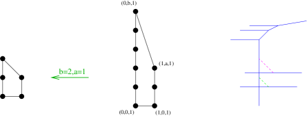
Figure 4: Toric diagram of $L^{aba}$ singularity in the case $a=2$, $b=5$, its dual diagram with the complex deformations, and its reduction to the $SPP$ toric diagram.

The $L^{aba}$ singularities contain ”$a$” conifold like singularities (hence ”$a$” conifold like complex deformations) and two lines of non isolated singularities passing through the tip of the cone: $\mathbb{C}^{2}/\mathbb{Z}_{a}$ and $\mathbb{C}^{2}/\mathbb{Z}_{b}$. Indeed the $L^{aba}$ singularities are described by a quadric in $\mathbb{C}^{4}$

$$x^{a}y^{b}=wz\,.$$ (11)

The lines parametrized by non zero values of $x$ and $y$ are the $\mathbb{C}^{2}/\mathbb{Z}_{b}$ and $\mathbb{C}^{2}/\mathbb{Z}_{a}$ non isolated singularities

$$x\neq 0\hbox{ }\rightarrow\hbox{ }y^{b}=wz\hbox{ }\hbox{ , }\hbox{ }y\neq 0\hbox{ }\rightarrow\hbox{ }x^{a}=wz\,.$$ (12)

We can deform the singularities (12) by inserting two cycles at the singular point. A generic $\mathbb{C}^{2}/\mathbb{Z}_{n}$ contains, indeed, $n-1$ two spheres collapsed at the origin and can be deformed to a smooth space turning on $n-1$ generic complex deformation parameters $\xi_{i}$, $i=1,...,n-1$

$$x^{n}=yz\rightarrow x\prod_{i=1}^{n-1}(x-\xi_{i})=yz\,.$$ (13)

On the other hand, from figure 4, we note that $L^{aba}$ contain $a$ conifolds that can be locally deformed as

$$xy-wz=0\hbox{ }\rightarrow\hbox{ }xy-wz-\epsilon_{j}=0\hbox{ , }\hbox{ }\hbox{ j=1,...a}\,.$$ (14)

We have thus identified two families of deformations: the $\xi$ deformations and the $\epsilon$ deformations. As already mentioned, we argue that the motion in the $\xi$ deformations breaks supersymmetry to a metastable vacuum, while the motion in the $\epsilon$ deformations restores it.

The gauge theories dual to these singularities [24, 25, 26] are non chiral and have the quiver representations in Figure 5.

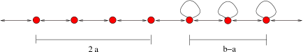
Figure 5: The quiver for the generic $L^{aba}$ singularity.

The theory has gauge group $U(N_{1})\times U(N_{2})\times...\times U(N_{a+b})$ and chiral fields transforming in the adjoint or in the bi-fundamental representations. The superpotentials are

$$W= \sum_{i=2a+1}^{b+a}X_{ii}(q_{i,i-1}q_{i-1,i}-q_{i,i+1}q_{i+1,i})+\sum_{j=1}^{2a}(-1)^{j+1}q_{j,j-1}q_{j-1,j}q_{j,j+1}q_{j+1,j}$$ (15)

where $a+b+1=1$ and the fields $X_{ii}$ transform in the adjoint representation of the i-th gauge group, while $q_{i,i+1}$ transform in the fundamental representation of the i-th group and in the anti-fundamental of the i+1-th group.

The chiral ring constrains of the gauge theory can be related to the algebraic geometric description of the singularity. The complex deformations can be mapped into deformations of the superpotential, as well. Indeed the equation (11) can be reconstructed through the supersymmetric constraints on the mesonic chiral ring of the gauge theory. Define the following set of basic mesonic chiral operators

$$x_{1}=q_{12}q_{21}\hbox{ }\hbox{ , }\hbox{ }x_{2}=q_{34}q_{43}\hbox{ }\hbox{ , }\hbox{ }\hbox{...}\hbox{ }\hbox{ , }\hbox{ }x_{a}=q_{2a-1,2a}q_{2a,2a-1};$$

$$y_{1}=q_{23}q_{32}\hbox{ }\hbox{ , }\hbox{ }y_{2}=q_{45}q_{54}\hbox{ }\hbox{ , }\hbox{ }\hbox{...}\hbox{ }\hbox{ , }\hbox{ }y_{a}=q_{2a,2a+1}q_{2a+1,2a},$$ (16)

$$y_{a+1}=q_{2a+1,2a+2}q_{2a+2,2a+1}\hbox{ }\hbox{ , }\hbox{ }\hbox{...}\hbox{ }\hbox{ , }\hbox{ }y_{b}=q_{b,1}q_{1,b};$$

$$X_{2a+1,2a+1}\hbox{ }\hbox{ , }\hbox{ }X_{2a+2,2a+2}\hbox{ }\hbox{ , }\hbox{ }\hbox{...}\hbox{ }\hbox{ , }\hbox{ }X_{b,b};$$

$$w=q_{1,b}q_{b,b-1}\hbox{ }\hbox{...}\hbox{ }q_{3,2}q_{2,1}\hbox{ }\hbox{ , }\hbox{ }z=q_{1,2}q_{2,3}\hbox{ }\hbox{...}\hbox{ }q_{b-1,b}q_{b,1}\,.$$ (17)

These operators satisfy

$$x_{1}...x_{a}\hbox{ }y_{1}...y_{b}=wz\,.$$ (18)

From the $F$-term equations we get the relations

$$x_{1}=...=x_{a}=X_{2a+1,2a+1}=...=X_{b,b}\hbox{ }\hbox{ , }\hbox{ }y_{1}=...=y_{b}\,.$$ (19)

The chiral ring constraints (18,19) reproduce the geometric singularity (11).

By this technique, using the $F$-term constraints, we can also map the complex deformations of the geometry to deformations of the superpotential.

A final, important, remark is that different UV gauge theories, flowing in the IR to the same conformal fixed point, correspond to the same toric singularity. These theories are related by Seiberg dualities and give equivalent physical descriptions at the conformal point. In this paper we choose the more convenient Seiberg phase for finding metastable vacua in the related non conformal case. This can be achieved by performing a set of Seiberg dualities on the quiver gauge theories with only regular branes, and then placing the right set of fractional branes that breaks conformal invariance.

3 Meta-stable vacua in $L^{aba}$ theories

This section is devoted to the analysis of metastability in the $L^{aba}$ theories with $b>a$. The simplest example is the one studied in [15], where the ISS dynamics dynamics was found in the infrared of a deformed $L^{121}$ theory. We now extend this analysis to more complicated cases, like $L^{131}$ and then $L^{1n1}$. After that we show how to generate chains of theories that have supersymmetry breaking meta-stable vacua. Generally speaking, if we have a $L^{aba}$ theory which shows metastability, we argue that the $L^{an,bn,an}$ theory behaves as a set of decoupled theories of this sort. At the end of this section, we give a general recipe for the existence of metastable vacua in a $L^{aba}$ theory, by decomposing it into a set of shorter quivers.

In the analysis of the metastable vacua we consider some nodes of the quivers as gauge groups and other nodes as flavor groups, tuning the dynamical scales as explained in the Appendix (B.1). This is implicit in all the cases that we treat.

Note that, in the notation of ISS, we are working in the magnetic description. This means that we deal with IR free gauge groups, without performing Seiberg duality on them. Another important remark is that, since we are dealing with the magnetic phase, if we want to realize metastable vacua, we need linear deformations in the mesons rather than massive quarks.

We present here several examples, as well as general results, to stress the fact that the $\xi$ deformations lead to metastable non supersymmetric vacua whereas the $\epsilon$ deformations bring to supersymmetry restoration. We leave the details of the field theory analysis in the Appendix D.

3.1 The $L^{131}$ theory

The $L^{131}$ theory is described by the quiver in figure 6,

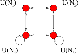
Figure 6: Quiver for the $L^{131}$ theory.

with superpotential

$$W= X_{33}(q_{32}q_{23}-q_{34}q_{43})-hq_{21}q_{12}q_{23}q_{32}+hq_{12}q_{21}q_{14}q_{41}+$$ (21)

$$+X_{44}(q_{43}q_{34}-q_{41}q_{14})$$

and it corresponds to the singular geometry

$$xy^{3}=wz$$ (22)

which is correctly reproduced by the mesonic chiral ring as explained in section 2.

We now add a superpotential deformation

$$W_{def}=-\xi_{1}(X_{33}-hq_{12}q_{21})-\xi_{2}(X_{44}-hq_{12}q_{21})\,.$$ (23)

Imposing the constraints from the $F$-term equations we find the new relations on the mesonic chiral ring

$$y=q_{23}q_{32}=q_{34}q_{43}+\xi_{1}=q_{41}q_{14}+\xi_{1}+\xi_{2}\,.$$ (24)

These constraints are translated into the deformed geometry

$$xy(y-\xi_{1})(y-\xi_{1}-\xi_{2})=wz\,.$$ (25)

Obviously, we are not obliged to add a linear term for each adjoint field but the case with only one deformation turns out to be unstable, as we show in the following.

We study this theory setting one node to zero. There are two different possibilities: we can set to zero a node with an adjoint field ($N_{3}$ or $N_{4}$) or a node without it ($N_{1}$ or $N_{2}$), obtaining a theory with one or two adjoint fields respectively. In the second case the scalar potential has dangerous flat directions and we cannot find metastable vacua. In the following we only analyze the first case and show the existence of long living non supersymmetric metastable vacua.

The theory under investigation is then obtained setting to zero the $N_{4}$ node (the case with $N_{3}=0$ is the same), described by the quiver in figure 7.

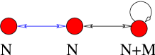
Figure 7: $L^{131}$ theory with $N_{4}=0$. The blue lines indicate massive matter.

The superpotential is

$$W=X_{33}q_{32}q_{23}-hq_{21}q_{12}q_{23}q_{32}-\xi_{1}X_{33}+h(\xi_{1}+\xi_{2})q_{21}q_{12}\,.$$ (26)

For simplicity, in the analysis of the equations of motion we fix the ranks of the groups to be

$$N_{1}=N_{2}=N\ \ \ \ \ N_{3}=N+M\,.$$ (27)

First of all we have to impose the correct tuning on the scales of the gauge groups and on the rank numbers in order to treat the node $N_{2}$ as an infrared free gauge group and the other gauge groups as flavours. Calculating the beta functions we have

$$b_{1}=2N\ \ \ \ b_{2}=N-M\ \ \ \ b_{3}=N+2M\,.$$ (28)

Since we require the group $U(N_{2})$ to be infrared free we impose the constraint $M>N$. Moreover, we require that this group is more coupled than the other groups at the supersymmetry breaking scale and at the scale of supersymmetry restoration. This can be done by tuning the scales $\Lambda_{1}$ and $\Lambda_{3}$, which are the strong coupling scales of two UV free gauge groups. Their scales have to be chosen much smaller than the scale of supersymmetry breaking (which is the deformation $h\xi_{1}$) and much smaller than the scale $\Lambda_{2}$ of $U(N_{2})$.

Now that we have correctly set up the role played by each gauge group in the quiver we can proceed in finding the vacua. A detailed analysis of this theory is left to the Appendix D.1. Here we sketch the main results. The $F$-term equation for the $X_{33}$ field is the rank condition and breaks supersymmetry, fixing the vev of the fields $q_{23}$ and $q_{32}$. The equation for the $q_{12}$ quark is

$$F_{q_{12}}=h\left(-q_{23}q_{32}+(\xi_{1}+\xi_{2})\right)q_{21}=h\xi_{2}q_{21}$$ (29)

and is solved with $q_{12}=0=q_{21}$. This is related to the fact that we have added two deformation parameters ($\xi_{1}$, $\xi_{2}$), i.e. two linear contributions to the superpotential for the two adjoint fields. Otherwise (for $\xi_{2}=0$), the equation (29) would be automatically satisfied, leaving the fields $q_{12}$ and $q_{21}$ unfixed at tree level and leading to potentially dangerous flat directions.

The non supersymmetric vacuum at tree level is

$$q_{12}=q_{21}^{T}=0\qquad q_{32}=q_{23}^{T}=\left(\begin{array}[]{c}\sqrt{\xi_{1}}\mathbf{1}_{N}\\ 0\end{array}\right)\qquad X_{33}=\left(\begin{array}[]{c c}0&0\\ 0&\chi\end{array}\right)$$ (30)

where $\chi$ is the pseudomodulus of dimension $M\times M$. As outlined in the Appendix D.1 this vacuum is stable under one loop correction, and the pseudomodulus is stabilized at $\chi=0$.

The restoration of supersymmetry is obtained in the hypothesis that the group labeled by $N_{2}$ develops a strong dynamics, by adding to the low energy superpotential a non perturbative contribution

$$W_{IR}=-\xi_{1}X_{33}+N_{2}\left(\Lambda^{3N_{2}-N_{3}}\det{X_{33}}\right)^{\frac{1}{N_{2}}}$$ (31)

where we have integrated out all the massive fields. From the geometric point of view, supersymmetry restoration, governed by the dynamics of the $U(N_{2})$ gauge group, can be described deforming the geometry with an $S^{3}$, i.e. an $\epsilon$ deformation,

$$(y-\xi_{1})(y-\xi_{1}-\xi_{2})(xy-\epsilon)=wz\,.$$ (32)

The low energy field theory superpotential (31) can be recovered from the geometric data (32). Indeed, setting $y=x^{\prime}-y^{\prime}$ and $x=x^{\prime}+y^{\prime}$, equation (32) becomes:

$$(x^{\prime}-y^{\prime}-\xi_{1})(x^{\prime}-y^{\prime}-\xi_{1}-\xi_{2})\left(x^{\prime}+\sqrt{y^{\prime 2}+\epsilon}\right)\left(x^{\prime}-\sqrt{y^{\prime 2}+\epsilon}\right)=wz\,.$$ (33)

The low energy superpotential can be written as a function of the glueball field $S_{2}$ (identified with $\epsilon/2$) and of the adjoint field $X_{33}$

$$W_{IR}(S_{2},X_{33})=W_{GVW}(S_{2})+W_{adj}(S_{2},X_{33})=N_{2}S_{2}\left(\log\frac{S_{2}}{\Lambda_{2}^{3}}-1\right)+\frac{t}{g_{2}}S_{2}+W_{adj}(S_{2},X_{33})\,.$$ (34)

Following the procedure explained in Appendix C the last term is derived from the geometric data

$$W_{adj}(S_{2},X_{33}) =\int({x^{\prime}}_{2}(y^{\prime})-{x^{\prime}}_{3}(y^{\prime}))dy^{\prime}=$$

$$=\int\left(y^{\prime}+{\xi_{1}}-\sqrt{y^{\prime 2}+\epsilon}\right)\sim\xi_{1}X_{33}-S_{2}\log\frac{X_{33}}{\Lambda_{m}}$$

where we have expanded the integral in the approximation $y^{\prime}\gg\xi_{1},\epsilon$. We can now solve the equation of motion for the glueball field $S_{2}$ and integrate it out, ignoring the multi-istanton contribution. In this way we recover from the geometry (32) the low energy superpotential (31).

As claimed in the introduction, we have shown, in this simple example, that the $\xi_{i}$ deformations lead to metastable vacua whereas the $\epsilon$ deformation leads to supersymmetry restoration.

3.2 The $L^{1n1}$ theories

The metastable $L^{131}$ theory can be generalized to the more complicate $L^{1n1}$ case. We find metastable supersymmetry breaking in the $L^{141}$ and $L^{151}$ theories and then we show how to extend this procedure to the $L^{1n1}$ case. A relevant aspect in the analysis is the decoupling between the breaking sector and the supersymmetric one. Once again we leave the details in the Appendix D, being here mainly interested in the geometrical realization of metastable supersymmetry breaking.

3.2.1 $L^{141}$

Here we study the quiver gauge theory of figure 8,

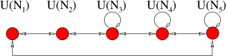
Figure 8: $L^{141}$ theory.

with superpotential

$$W= hq_{12}q_{23}q_{32}q_{21}-X_{33}q_{32}q_{23}+X_{33}q_{34}q_{43}-X_{44}q_{43}q_{34}$$ (36)

$$X_{44}q_{45}q_{54}-X_{55}q_{54}q_{45}+X_{55}q_{51}q_{15}-hq_{51}q_{12}q_{21}q_{15}\,.$$

The geometry associated with this theory is described by the equation

$$xy^{4}=wz\,.$$ (37)

Supersymmetry breaking is driven by linear terms for the adjoint fields. We add the deformation superpotential

$$W_{\text{def}}=-\xi_{3}(X_{33}-hq_{32}q_{23})+\xi_{4}(X_{44}-hq_{32}q_{23})\ -\xi_{5}(X_{55}-hq_{32}q_{23})\,.$$ (38)

We have add a linear term for all the adjoint fields: this is crucial for the stability of the non supersymmetric vacuum. The $q_{23}$ and $q_{32}$ quarks become massive, since the $F$-terms constraints have to be compatible.

The corresponding geometry reads now

$$x(y-\xi_{3})(y-\xi_{3}-\xi_{4})(y-\xi_{3}-\xi_{4}-\xi_{5})y=wz\,.$$ (39)

If we consider as gauge group the node $U(N_{2})$ and choosing the ranks as

$$N_{1}=N_{2}=N_{5}=N\quad N_{3}=N+M\quad N_{4}=0$$ (40)

with $M>N$, this theory breaks supersymmetry through rank condition for the meson $X_{33}$. A detailed analysis (see Appendix D.2) shows that this theory possesses metastable vacua without dangerous flat directions.

Two important remarks are in order. Without turning on the deformation $\xi_{4}$ (the one related to the node set to zero) we are not protected from instabilities of the scalar potential (see Appendix D.2). Furthermore, as we did in the $L^{131}$ case, we have decoupled an ISS like sector with supersymmetry breaking from a supersymmetric sector. These two facts hold in all the $L^{1n1}$ cases.

The process of supersymmetry restoration works as in the $L^{131}$, when the dynamics of the gauge group $U(N_{2})$ gives rise to non perturbative contributions to the superpotential.

3.2.2 $L^{151}$

Here we study metastability in the $L^{151}$ quiver gauge theory. This is the basic example for the generalization of the analysis to the $L^{1n1}$ case.

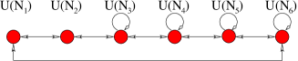
Figure 9: The $L^{151}$ theory.

The gauge theory, related to the quiver in figure 9, has superpotential

$$W= hq_{12}q_{23}q_{32}q_{21}-X_{33}q_{32}q_{23}+X_{33}q_{34}q_{43}-X_{44}q_{43}q_{34}+X_{44}q_{45}q_{54}$$ (41)

$$-X_{55}q_{54}q_{45}+X_{55}q_{51}q_{15}-X_{66}q_{65}q_{56}+X_{66}q_{61}q_{16}-hq_{61}q_{12}q_{21}q_{16}$$

and it is associated to the geometry

$$xy^{5}=wz\,.$$ (42)

Once again we deform the superpotential with linear terms for the adjoint fields and masses for the quarks

$$W_{\text{def}}=-\xi_{3}(X_{33}-hq_{32}q_{23})-\xi_{4}(X_{44}-hq_{32}q_{23})-\xi_{5}(X_{55}-hq_{32}q_{23})-\xi_{6}(X_{66}-hq_{32}q_{23})\,.$$ (43)

The deformation (43) leads to the geometric deformation

$$x(y-\xi_{3})(y-\xi_{3}-\xi_{4})(y-\xi_{3}-\xi_{4}-\xi_{5})(y-\xi_{3}-\xi_{4}-\xi_{5}-\xi_{6})y=wz\,.$$ (44)

We choose the ranks of the groups as

$$N_{1}=N_{2}=N_{5}=N_{6}=N\qquad N_{3}=N+M\qquad N_{4}=0$$ (45)

with $M>N$. The equation of motion for the field $X_{33}$ is the ISS rank condition, that breaks supersymmetry at the classical level. In the Appendix D.3 we show that the supersymmetry breaking minimum is stable. Stability of the metastable vacuum requires $\xi_{3},\xi_{4},\xi_{5}\neq 0$ and arbitrary $\xi_{6}$.

The supersymmetry restoration carries on exactly as in the $L^{131}$, with non perturbative contribution to the superpotential due to the dynamics of the gauge group $U(N_{2})$.

3.2.3 $L^{1n1}$

We now extend the results about metastability to the general $L^{1n1}$ theory. The superpotential is

$$W= \sum_{i=3}^{n}X_{i,i}(q_{i,i-1}q_{i-1,i}-q_{i,i+1}q_{i+1,i})+hq_{21}q_{12}q_{23}q_{32}-hq_{12}q_{21}q_{1,n+1}q_{n+1,1}+$$ (47)

$$+X_{n+1,n+1}(q_{1,n+1}q_{n+1,1}-q_{n,n+1}q_{n+1,n})$$

and the geometry

$$xy^{n}=wz\,.$$ (48)

The deformation of the superpotential is

$$\Delta W=\sum_{i=3}^{n+1}\xi_{i}(hq_{12}q_{21}-X_{i,i})$$ (49)

which corresponds to the geometry

$$xy\prod_{i=3}^{n+1}(y-\sum_{j=1}^{i}\xi_{i})=wz\,.$$ (50)

We choose the ranks of the nodes to be

$$N_{4}=0\qquad N_{3}=N+M\qquad N_{j}=N\quad(j\neq 3,4)$$ (51)

such that supersymmetry is broken at node 3. Moreover it should be $M>N$ for $U(N_{2})$ to be IR free.

The deformations $\xi_{3}$, $\xi_{4}$ and $\xi_{5}$ have to be different from zero for the non supersymmetric vacuum to be stable. All the other deformations can be chosen arbitrarily (see Appendix D.4). The breaking sector is the same than all the other $L^{1n1}$ cases analyzed before. The only difference is that the supersymmetric sector is larger here.

Supersymmetry is restored by the strong dynamics of the gauge group $U(N_{2})$, and the metastable vacuum is long living. This concludes the analysis of the $L^{1n1}$ theories.

3.3 Extension to longer quivers

We extend here the analysis of the $L^{1n1}$ theories to more complicated $L^{aba}$ cases. The strategy is to decouple an $L^{aba}$ theory in a set of $a$ metastable theories, adding $b-a$ deformations, one for each adjoint field. In the case $b-a\geq a$ ,by using the results obtained for $L^{1n1}$, we are able to find metastable vacua in each $L^{aba}$ theory.

Our general strategy will be to consider in each metastable subset only one group as a gauge group, since there are some difficulties in treating the dynamics of more than one gauge group simultaneously.

We study first the simplest cases, like the $L^{n2nn}$ theory, which can be viewed as a set of decoupled ISS models. This is a pedagogical example, useful for the extension of the analysis to the general situations and for the proof that metastability is a generic phenomenon in the $L^{aba}$ theories. At the end of this subsection, we furnish the general recipe to build metastable $L^{aba}$ quivers.

3.3.1 $L^{n2nn}$ as a set of decoupled ISS

The $L^{121}$ gauge theory, in the ISS regime, has been shown to possess meta-stable vacua [15]. Starting from an $L^{n2nn}$ quiver gauge theory we can perform a set of Seiberg dualities going from the first quiver in the Figure 10 to the second one. In fact, Seiberg duality on these theories has the effect of displacing the adjoint fields. Each duality moves one adjoint field two nodes farther.

(a)

(b)

Figure 10: Two different Seiberg phases of the same $L^{363}$ quiver gauge theory.

We now deform the geometry, associating each $\xi_{i}$ deformation with the $i$-th node, obtaining

$$\prod_{i=1}^{n}x(y-\xi_{3i-2})y=wz\,.$$ (52)

This deformation corresponds, on the gauge side, to the combined addition of linear terms for the adjoint fields and of masses for the appropriate bifundamentals (i.e. that ones not directly coupled to the adjoint fields). By setting to zero one node, without an adjoint field, every three nodes, we have a theory of decoupled metastable ISS models (see Figure 11).

Figure 11: $L^{363}$ as a set of three decoupled ISS models

The analysis of metastable vacua is the same as in ISS for each sector. Supersymmetry is restored in the large field region in each ISS sector, where the gauge group gives rise to a non perturbative contribution in the effective theory. The non perturbative contributions modify the constraints on the mesonic moduli space, and hence the geometry, as

$$\prod_{i=1}^{n}y\left((y-\xi_{3i-2})x-\epsilon_{i}\right)=wz\,.$$ (53)

The technique of Appendix C can be applied to the new singularities of the geometry to recover the correct low energy behavior of the field theory. The calculation proceeds exactly as in the $L^{121}$ case

3.3.2 The $L^{n3nn}$ theories

With this strategy we can build longer quivers with metastable vacua. For example the $L^{131}$ case can be extended to metastable $L^{n3nn}$ theories. Indeed we can perform a set of Seiberg dualities to obtain a new phase of the theory as shown in Figure 12.

(a)

(b)

Figure 12: Two different Seiberg phases of the same $L^{393}$ quiver gauge theory.

As we did in the $L^{n2nn}$ case, we then deform the geometry

$$\prod_{i=1}^{2n}(y-\xi_{4(i-1)}-\xi_{4(i+1)+1})yx(y-\xi_{4i})=wz\ \ \ \ \ \ \ \ \ \ \ \text{with}\ \ \ \xi_{0}=\xi_{4n}\,.$$ (54)

The deformation brings in the superpotential a linear term for each adjoint field, and a mass term for the quarks stretched between two nodes without the adjoint fields.

We set then to zero the right nodes and breaks the $L^{n3nn}$ into a set of metastable gauge theories. Indeed, setting the ranks number as in Figure 13,

Figure 13: $L^{393}$ as a set of three decoupled $L^{131}$ models.

in each decoupled sector we have the same breaking patterns as in the $L^{131}$ studied before. Each sector has the superpotential

$$W=hq_{i,i+1}q_{i+1,i+2}q_{i+2,i+1}q_{i+1,i}\ -q_{i+1,i}X_{i,i}q_{i,i+1}-\xi_{i}X_{i,i}+h(\xi_{i}+\xi_{i+3})q_{i+2,i+1}q_{i+1,i+2}$$ (55)

which leads to long living metastable vacua, as it has been explained for the $L^{131}$ theory.

Supersymmetry restoration can be obtained separately in each decoupled sector, through the strong dynamics of the gauge group. In the geometric description it can be read from the deformation of the variety

$$\prod_{i=1}^{2n}\left((y-\xi_{4(i-1)}-\xi_{4i-3})x-\epsilon_{i}\right)y(y-\xi_{4i})=wz\,.$$ (56)

It is straightforward to show that it corresponds to adding a term proportional to $\det X_{ii}$ for each gauge group and restores supersymmetry.

3.3.3 Extension with an example

The procedure just outlined for the $L^{121}$ and $L^{131}$ can be applied also for the $L^{1n1}$ case, extending it to $L^{m,nm,m}$ metastable theories.

More generally, we can consider an $L^{aba}$ quiver that can be decomposed into subsets of different theories, each one metastable.

We show the technique in a clarifying example and then give a general recipe. For instance, we take the $L^{252}$ theory and perform a Seiberg duality to obtain the phase of figure 14.

Figure 14: The Seiberg phase of $L^{252}$ suitable for metastable vacua

By deforming all the adjoint fields with a linear term the chiral ring gets modified to be

$$y=q_{23}q_{32}=q_{34}q_{43}+\xi_{3}=q_{56}q_{65}=q_{67}q_{76}+\xi_{6}=q_{71}q_{17}+\xi_{6}+\xi_{7}$$

$$x=q_{12}q_{21}=q_{45}q_{54}$$ (57)

with the corresponding deformed geometry

$$x^{2}y^{2}(y-\xi_{3})(y-\xi_{6})(y-\xi_{6}-\xi_{7})=wz\,.$$ (58)

We choose then the sequence of the ranks of the groups as shown in figure 14, setting to zero the fourth and the last node. Now the first sector corresponds to the $L^{131}$ theory and the second one to the $L^{121}$ one. Each sector shows metastable supersymmetry breaking vacua. The superpotential is

$$W=hq_{12}q_{23}q_{32}q_{21}-q_{23}X_{33}q_{32}-q_{56}X_{66}q_{65}-\xi_{3}X_{33}-\xi_{6}X_{66}+(\xi_{3}+\xi_{7})q_{21}q_{12}\,.$$ (59)

Supersymmetry is restored by the strong dynamics of the nodes two and five that give rise to the non perturbative contribution

$$W_{\text{dyn}}=N\left(\Lambda_{2}^{2N-M}\det X_{33}\right)^{1/N}+N\left(\Lambda_{5}^{2N-M}\det X_{66}\right)^{1/N}$$ (60)

which deforms the geometry to

$$(xy-\epsilon_{1})(xy-\epsilon_{2})(y-\xi_{3})(y-\xi_{6})(y-\xi_{6}-\xi_{7})=wz\,.$$ (61)

Indeed, from this geometry, with the technique discussed in the Appendix C, we can recover now the low energy superpotential of the field theory.

We start writing the general $IR$ superpotential as a function of the mesons $X_{33}$ and $X_{66}$ and of the glueballs $S_{2}$ and $S_{5}$

$$W_{IR}=W_{GVW}(S_{2})+W_{GVW}(S_{5})+W_{adj}(S_{2},X_{33})+W_{adj}(S_{5},X_{66})\,.$$ (62)

Substituting $y=x^{\prime}-y^{\prime}$ and $x=x^{\prime}+y^{\prime}$ in (61) we can calculate the contributions $W(S,X)$ in the superpotential

$$W_{adj}(S_{2},X_{33}) = \int\left(y^{\prime}+\xi_{3}-\sqrt{{y^{\prime}}^{2}+\epsilon_{1}}\right)dy^{\prime}\sim\xi_{3}X_{33}-S_{2}\log{\frac{X_{33}}{\Lambda_{2}}}$$

$$W_{adj}(S_{5},X_{66}) = \int\left(y^{\prime}+\xi_{6}-\sqrt{{y^{\prime}}^{2}+\epsilon_{2}}\right)dy^{\prime}\sim\xi_{6}X_{66}-S_{5}\log{\frac{X_{66}}{\Lambda_{5}}}$$ (63)

where we identify $(2S_{2},2S_{5})=(\epsilon_{1},\epsilon_{2})$. We remark that the variable $y^{\prime}$, that parametrizes the position of the brane, can be interpreted as the vev of the field $X_{ii}$ in each integral. Integrating out the glueball fields $S_{2}$ and $S_{5}$ we recover the low energy description of the field theory.
This example shows that we can obtain metastable $L^{aba}$ theories by breaking them up into shorter quivers.

3.3.4 General analysis

Here we decompose an $L^{aba}$ theory into a set of $L^{1n_{i}1}$ theories, each one with metastable vacua.

We consider a distribution of gauge groups with ranks such that there are no consecutive nodes set to zero. Moreover we consider only Seiberg phases with $b-a$ adjoint fields to be distributed on the $a$ gauge nodes. This implies that we can only describe theories with $b-a\geq a$. In the next section we extend this result to theories with $b-a<a$, studying Seiberg phases with more adjoint fields.

With these assumptions, starting from a $L^{aba}$ and setting $a$ nodes to zero, we can obtain $a$ metastable $L^{1n_{i}1}$ theories. Each decoupled sector possesses long living metastable vacua like the ones studied in the $L^{1n_{i}1}$ theories and hence the whole theory is metastable. The procedure is not unique: we can indeed decouple the $L^{aba}$ theory in different sets of $L^{1n_{i}1}$ quivers. This is related to the fact that we can distribute differently the $b-a$ adjoint fields on the $a$ gauge nodes and set to zero nodes with or without adjoint fields.

This can be shown in a simple example. The $L^{383}$ theory can be decoupled in three different sectors, where the number of adjoint fields totals up to five. There are two inequivalent possibilities to obtain metastable vacua as shown in figure 15.

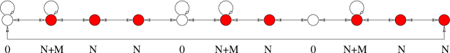
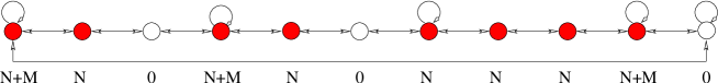
Figure 15: The two inequivalent possible $L^{383}$ that give rise to three decoupled metastable sectors

We set three different nodes to zero (nodes $1,5,8$ in the first case and $3,6,11$ in the second one), obtaining three decoupled metastable theories. For the first case the analysis of metastability follows from $L^{121}$ and $L^{131}$, while in the second case it follows from $L^{121}$ and $L^{141}$. So we decouple $L^{383}$ in two different ways: as $2L^{131}+L^{121}$ or as $2L^{121}+L^{141}$. By this technique, we can write $L^{aba}$ as a sum of $\sum_{i=1}^{a}L^{1n_{i}1}$, with the constraint $\sum_{i=1}^{a}n_{i}=b$, $n_{i}\geq 2$. All these theories lead, with the right distribution of ranks, to metastable vacua.

4 Meta-stable vacua in $L^{aaa}$ theories

In the case $a=b$, i.e. $L^{aaa}$ the theory does not posses adjoint matter, since $b-a=0$. Nevertheless, by performing Seiberg dualities, we can create the necessary adjoint fields. As explained at the end of section 2, this procedure does not affect the geometry, which is of the form

$$x^{a}y^{a}=wz\,.$$ (64)

We can then add the deformations for the adjoint fields and obtain theories suitable for metastable supersymmetry breaking.

Once again the strategy to analyze a long quiver consists in breaking it up in a set of shorter quivers, each one with metastable vacua.

We study in detail the simplest example, $L^{222}$, and then we comment on possible generalizations.

4.1 The $L^{222}$ theory

We analyze here the $L^{222}$ theory after a Seiberg duality. The quiver of the complete theory (see figure 16) is related to the double conifold. The superpotential is

Figure 16: The $L^{222}$ quiver without any node set to zero

$$W=-q_{21}X_{11}q_{12}+hq_{12}q_{23}q_{32}q_{21}-q_{23}X_{33}q_{32}+q_{41}X_{11}q_{14}-hq_{14}q_{43}q_{34}q_{41}+q_{43}X_{33}q_{34}$$ (65)

and the geometry is given by the equation

$$x^{2}y^{2}=wz\,.$$ (66)

We deform the geometry

$$x(y-\xi_{1})y(x-\xi_{3})=wz\,.$$ (67)

This deformation changes the constraints on the mesonic chiral ring. The new constraints can be satisfied by adding in $W$ two linear terms of the form $\xi_{1}X_{11}$ and $\xi_{3}X_{33}$, and we have to switch on also two mass terms in the quarks fields. Setting to zero one node, we can have the three different cases, as shown in figure 17.

Figure 17: Three different quivers from the deformed $L^{222}$. The massive quarks are represented with blue lines, the massless quarks are represented with black lines.

They all have metastable vacua in the correct regime of couplings, ranks and scales.

These models are similar to ISS, but with two differences: the quartic term for the quarks and the mass term for some of the quarks.

We study here the case with only one group of massive quarks (the first case in the figure 17), and then we comment on the other at the end of this paragraph. A detailed analysis that includes the three cases, for generic values of the masses of the quarks, is in the Appendix D.5.

We choose the ranks of the groups to be

$$N_{2}=N\ \ \ \ N_{1}=N+M=N_{3}\,.$$ (68)

The second node is treated as the gauge group and the other two nodes as flavours. The superpotential is

$$W=-(\xi_{1}X_{11}+\xi_{3}X_{33})-q_{21}X_{11}q_{12}+hq_{12}q_{23}q_{32}q_{21}-q_{23}X_{33}q_{32}+h\xi_{1}q_{32}q_{23}\,.$$ (69)

We then solve the equations of motion for the various fields, recognizing the ISS rank condition, responsible for breaking of supersymmetry. The $F$-terms fix the vacuum to be

$$q_{12}=q_{21}^{T}=\left(\begin{array}[]{c}\sqrt{\xi_{1}}\\ 0\end{array}\right)\ \ \ \ q_{32}=q_{23}^{T}\left(\begin{array}[]{c}\sqrt{\xi_{3}}\\ 0\end{array}\right)\ \ \ \ X_{11}=\left(\begin{array}[]{cc}0&0\\ 0&\chi_{1}\end{array}\right)\ \ \ \ X_{33}=\left(\begin{array}[]{cc}\xi_{1}&0\\ 0&\chi_{3}\end{array}\right)\,.$$ (70)

In the Appendix D.5 we show that this vacuum is stable up to one loop corrections, fixing the pseudomoduli to $\langle\chi_{1}\rangle=0$ and $\langle\chi_{3}\rangle=\xi_{1}$. The two breaking sectors are separated at the one loop level, and their quantum corrections are as in ISS. The $\xi_{i}$ deformations have thus lead to supersymmetry breaking vacua.

The strong dynamics of the gauge group restores supersymmetry, and is geometrically described by the $\epsilon$ deformation

$$(x-\xi_{1})\left(x(y-\xi_{3})-\epsilon\right)y=wz\,.$$ (71)

In the field theory analysis we explore the large field region for the mesons, by integrating out the massive fields, and by taking into account the non perturbative contributions due to gaugino condensation. The low energy superpotential results

$$W_{IR}=N\left(\Lambda^{-2M-N}\det{X_{11}}\det{X_{33}}\right)^{\frac{1}{N}}-\left(\xi_{1}{\rm Tr}X_{11}+\xi_{3}{\rm Tr}X_{33}\right)$$ (72)

which guarantees the long life of the vacuum.

On the other hand, we can use the geometric techniques of Appendix C to recover the same low energy superpotential (72) from the geometry (71). Relabeling the variables in (71) by $y=(x^{\prime}-y^{\prime})$ and $x=(x^{\prime}+y^{\prime})$ we can rewrite

$$(x^{\prime}-y^{\prime}-\xi_{1})\left((x^{\prime}-y^{\prime})((x^{\prime}+y^{\prime}-\xi_{3})-\epsilon\right)=wz\,.$$ (73)

The geometric superpotential is

$$W_{IR}(S,X_{11},X_{33})=N_{2}S\left(\log\frac{S}{\Lambda^{3}_{m}}-1\right)-\frac{t}{g}S+W_{adj}(S,X_{11})+W_{adj}(S,X_{33})\,.$$ (74)

The two contributions $W_{adj}$ derive from the singularities of the geometry. Repeating the computations as in Appendix C we have

$$W_{adj}(S,X_{11})= \int\left(y^{\prime}+\xi_{1}-\frac{\xi_{3}}{2}-\sqrt{\left(y^{\prime}-\frac{\xi_{3}}{2}\right)^{2}+\epsilon}\right)dy^{\prime}$$

$$W_{adj}(S,X_{33})= \int\left(\frac{\xi_{3}}{2}-\sqrt{\left(y^{\prime}-\frac{\xi_{3}}{2}\right)^{2}+\epsilon}+y^{\prime}\right)dy^{\prime}\,.$$ (75)

In the previous integral we identify $2S$ with $\epsilon$ and $y^{\prime}$ with the vev of the adjoint fields $X_{11}$ and $X_{33}$ respectively. In the regime $y^{\prime}\gg\epsilon,\xi_{i}$ we can compute the integrals expanding at first order in $\epsilon$ and $\xi_{i}$, obtaining the superpotential for the interaction between the glueball field and the adjoint fields

$$W_{adj}(S,X_{11})+W_{adj}(S,X_{33})=\xi_{1}{\rm Tr}X_{11}+\xi_{3}{\rm Tr}X_{33}-S\log\det\left(\frac{X_{11}}{\Lambda_{m}}\right)-S\log\det\left(\frac{X_{33}}{\Lambda_{m}}\right)\,.$$ (76)

The equation for the glueball field $S$ can be derived from (74) and (76). Solving for $S$ and ignoring the multi-istanton contributions we have

$$S=\left(\Lambda_{m}^{3N_{2}-N_{1}-N_{3}}\det{X_{11}}\det{X_{33}}\right)^{\frac{1}{N_{2}}}=\left(\Lambda_{m}^{-N-2M}\det{X_{11}}\det{X_{33}}\right)^{\frac{1}{N}}\,.$$ (77)

Substitution of (77) in (74) gives the same low energy superpotential of field theory (72), up to an overall sign.

The $\epsilon$ deformation has lead to supersymmetry restoration.

4.2 The $L^{333}$ theory

Here we search for metastable vacua in an $L^{333}$ theory, after performing on it some Seiberg dualities. This theory has six nodes without adjoint fields, with superpotential

$$W=\sum_{i=1}^{4}(-1)^{i}hq_{i,i+1}q_{i+1,i+2}q_{i+2,i+1}q_{i+1,i}-hq_{56}q_{61}q_{16}q_{65}+hq_{61}q_{12}q_{21}q_{16}\,.$$ (78)

A Seiberg duality on the sixth node and integration out of the massive matter. leads to the superpotential

$$W= -q_{61}X_{11}q_{16}+q_{21}X_{11}q_{12}-hq_{12}q_{23}q_{32}q_{21}+hq_{23}q_{34}q_{43}q_{32}-hq_{34}q_{45}q_{54}q_{43}$$ (79)

$$+q_{45}X_{55}q_{54}-q_{65}X_{55}q_{56}+hq_{56}q_{61}q_{16}q_{65}$$

with the quiver given in figure 18.

Figure 18: The $L^{333}$ theory after a Seiberg duality on node $6$.

The geometry is then deformed by the $\xi_{i}$ terms to

$$x^{2}y^{2}(y-\xi_{1})(x-\xi_{5})=wz\,.$$ (80)

This deformation corresponds in the field theory to linear terms $\xi_{1}X_{11}$ and $\xi_{5}X_{55}$ in the superpotential. For consistency with the $F$-term constraints, we also add some mass term for the bifundamentals, i.e.

$$\Delta W=-\xi_{1}X_{11}+\xi_{5}X_{55}+h\xi_{1}q_{23}q_{32}-h\xi_{5}q_{43}q_{34}\,.$$ (81)

We set the ranks of the groups as follows

$$N_{1}=N_{5}=N+M\qquad N_{2}=N_{4}=N\qquad N_{3}=N_{6}=0\,.$$ (82)

We then obtain two decoupled ISS like models that break supersymmetry through rank conditions for the mesons $X_{11}$ and $X_{55}$.

The supersymmetric vacua can be recovered by adding the non perturbative contributions arising for each gauge group. From the geometry, restoration of supersymmetry can be described by the $\epsilon_{i}$ deformations

$$xy(x(y-\xi_{1})+\epsilon_{1})((x-\xi_{5})y-\epsilon_{2})=wz\,.$$ (83)

This deformed geometry gives, with the techniques of Appendix C, the right low energy superpotential that leads to the supersymmetric vacua.

4.3 Extension

We now briefly outline a procedure for finding metastable vacua in a generic $L^{aaa}$ theory.

The strategy again consists in breaking the quiver into a set of shorter quivers, each one metastable.

We study a phase of the theory, derived by acting with Seiberg dualities, which has a number of $a$ adjoint fields if $a$ is even and $a-1$ if $a$ is odd.

We then set to zero the right nodes in order to obtain a set of decoupled theories that have the same structure of the deformed $L^{222}$ and $L^{333}$ studied above. This can be done choosing appropriately the Seiberg phases.

We now show how to proceed in a simple example, $L^{555}$ in figure 19.

Figure 19: Quiver for the deformed $L^{555}$ theory.

We perform Seiberg dualities on the sixth and on the tenth node and obtain $4$ adjoint fields. We then deform the geometry in such a way that, in the field theory description, all the adjoint fields get linear terms

$$x^{3}y^{3}(y-\xi_{1})(x-\xi_{5})(y-\xi_{7})(x-\xi_{9})=wz\,.$$ (84)

Indeed, this deformation give rise to linear terms for all the adjoint fields, and masses for some of the quarks. The new superpotential contribution is

$$\Delta W=\xi_{1}q_{23}q_{32}+\xi_{5}q_{34}q_{43}+\xi_{7}q_{56}q_{65}+\xi_{9}q_{110}q_{101}-\xi_{1}X_{11}-\xi_{5}X_{55}-\xi_{7}X_{77}-\xi_{9}X_{99}\,.$$ (85)

We now set to zero the third, the sixth and the tenth node. In this way we decompose the theory in three different metastable sectors. The first two sectors have the same structure of $L^{333}$, whereas the last sector is like the theory emerging from a $L^{222}$. In short we have decomposed the $L^{555}$ as $L^{222}$ and $L^{333}$.

Supersymmetry restoration is achieved in each sector separately. From the geometric point of view this transition is read as an $\epsilon$ deformation of (84) to

$$x^{2}y^{2}((y-\xi_{1})x-\epsilon_{1})(y(x-\xi_{5})-\epsilon_{2})((y-\xi_{7})(x-\xi_{9})-\epsilon_{3})=wz$$ (86)

where the three $\epsilon_{i}$ take into account the deformations on the moduli space imposed by the strong dynamics of the three groups that we considered as gauge groups. Using the geometric techniques of Appendix C it is possible also in this case to recover the correct low energy behavior in the supersymmetric vacua. The three different deformation parameters $\epsilon_{i}$ are interpreted as the three glueball fields of the three gauge groups.

4.4 Back to $L^{aba}$

Up to now we have found metastable vacua in all the $L^{aaa}$ theories (with $a>1$) and in $L^{aba}$ with the constraint $b-a>a$. The study of the $L^{aaa}$ theories gives us a way out from the constraints imposed on $L^{aba}$. If we have an $L^{aba}$ theory with $b-a<a$ we have indeed to look for a different Seiberg phase. Given an $L^{aba}$ theory one can find a dual theory with at most $b+a-2$ adjoint fields, instead of $b-a$.

We proceed in a simple example: the $L^{343}$ theory. A Seiberg duality on the fourth node gives the quiver in figure 20.

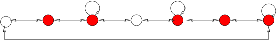
Figure 20: $L^{343}$ theory with a Seiberg duality on the fourth node.

By adding a linear deformation for each adjoint field, the geometry becomes

$$x^{2}y^{2}(y-\xi_{1})(x-\xi_{2})(y-\xi_{3})=wz\,.$$ (87)

We can now set some node to zero and obtain a set of decoupled theories with a metastable IR behavior. A possible choice is shown in figure 20, where we set to zero the white nodes. We have broken up $L^{343}$ theory in two sectors: the first one has the same property of metastability of $L^{121}$, and the second one of $L^{222}$, the double conifold.

Supersymmetry is restored by the geometric $\epsilon$ deformation

$$xy((y-\xi_{1})x-\epsilon_{1})(x-\xi_{2})(xy-\epsilon_{2})(y-\xi_{3})=wz$$ (88)

through the strong dynamics of the gauge group in each decoupled sector.

5 Beyond the $L^{aba}$ cases

In the previous sections we performed metastable supersymmetry breaking in the family of $L^{aba}$ singularities. An immediate generalization is the embedding of $L^{aba}$ in larger singularities and the recovering of metastable dynamics in the IR.

We need to start with a UV quiver gauge theory and flow by way of the renormalization group to a set of gauge theories with fewer gauge groups. These theories are decoupled at low energy, and they keep at least one $L^{aba}$ singularity. These singularities trigger metastability in the IR.

In the RG flow to the IR two different decouplings are possible, the resolution and the deformation of the mother singularity.
Blowing up two spheres gives first the resolution of the mother singularity. The daughters singularities are geometrically separated by the volume of these two spheres. This corresponds to the motion in the Kahler moduli space of the singularities.
The second one, the deformation, is achieved by blowing-up three spheres. Here the singularities are separated by the volume of the three spheres.
In both cases the IR theories decouple at the level of massless states and the masses of the messenger fields are controlled by the volume of the two and three spheres respectively.
We now describe these two possibilities by proceeding with pictures and examples.

The graphical resolution of a singularity in the toric language corresponds to drawing a line in the toric diagram (the red line in our figures) and a perpendicular line in the dual diagram (the dashed line). This last line parametrizes the volume of the two sphere (see Figure 21).

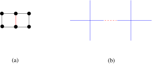
Figure 21: The toric resolution of the double conifold: $L^{222}$. (a) The toric diagram representation, (b) the dual diagram: the broken red arrow parametrize the volume of the blown up two sphere.

A natural laboratory for these constructions is the family of Pseudo del Pezzo singularities $PdP_{n}$. These are complex cones over $\mathbb{P}^{2}$, blown up at $n$ non-generic points. This blowing up generates lines of singularities passing trough the tip of the cones (Figure 22).

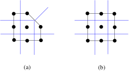
Figure 22: The toric diagrams and the dual diagrams for (a) $PdP_{4}$ and (b) $PdP_{5}$.

In the $PdP_{4}$ and $PdP_{5}$ singularities it is possible to recover two of the singularities that show a metastable behavior, $L^{121}$ ($SPP$) and $L^{222}$ (double conifold), through the resolution of the singularities as shown in Figure 23.

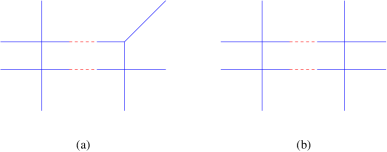
Figure 23: Resolutions of (a) $PdP_{4}$ and (b) $PdP_{5}$.

We first assign a set of fractional branes to the mother singularity such that it reproduces, at least for one of the daughter singularities, the set of fractional branes that has metastable non supersymmetric vacua. We turn then on Kahler moduli deformations, decoupling in the IR one $L^{121}$ and one $L^{222}$ singularities from the $PdP_{4}$. For the $PdP_{5}$ singularity we can decouple two $L^{222}$ singularities. In each situation the two decoupled IR theories are separated at the level of massless states . Finally, metastable supersymmetry breaking can be realized, since we can deform the $A_{1}$ singularities belonging to one or to both the IR theories.

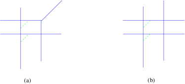
Figure 24: Deformations of (a) $PdP_{4}$ and (b) $PdP_{5}$.

The other possibility for the decoupling of a mother singularity is the deformation (see section 2 for a graphical description). It furnishes a second embedding of $L^{121}$ and $L^{222}$ into $PdP_{4}$ and $PdP_{5}$. These configurations are described in Figure 24.

We have to distribute the fractional branes at the mother singularity in such a way that they lead to the complex moduli deformation. Gaugino condensation is then induced by the strong dynamics of some gauge groups. This decoupling leads to the remaining daughter singularities in the IR, and, in this case, we are left with $L^{121}$ and $L^{222}$. We can move in the complex moduli space deformations of the non local singularity, reproducing the supersymmetry breaking behaviour of the $L^{aba}$ theories.
The advantage of this procedure is that the moduli associated with the volumes of the three spheres are automatically stabilized by the strong IR gauge dynamics. The drawback is that the computation of the masses of the messenger sector is not straightforward.

Following the two procedures explained in this section and the methods developed in [28] many examples, useful for model building, can be studied.

There exist conical singularities that provide extensions of MSSM as the IR limit of the dynamics of D3 branes put at the tip of the cone. The easiest example is given by $D3$ branes at $dP_{0}$ singularity.

Here, by using either Kahler moduli deformations or complex moduli deformations, it is possible to separate a singularity into a $dP_{0}$ sector and some $L^{aba}$ sector. In the IR, $dP_{0}$ is an extension of the MSSM, $L^{aba}$ is the hidden supersymmetry breaking sector, and the massive fields are the messengers. It is possible to find many examples of singularities that, after the resolution, decouple in a MSSM like sector and in a hidden supersymmetry breaking sector, also metastable. We show here two possibilities.

The first one, in Figure 25, admits a resolution that decouples in the IR a $dP_{0}$ and two $SPP$ singularities. The $dP_{0}$ plays the role of phenomenological sector, while the two $SPP$ singularities play the role of supersymmetry breaking hidden sectors. The second one, in figure 26, admits a complex deformation. It decouples a $dP_{0}$ sector and a single $SPP$ sector.

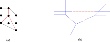
Figure 25: The resolved toric diagram (a) and the dual diagram (b). The triangle at the bottom is the $dP_{0}$ singularity that represents the “visible sector”, the polygon on the top are two decoupled SPP singularities that represent the supersymmetry breaking sector.

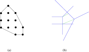
Figure 26: (a) The toric diagram of the mother singularity and (b) the deformed dual diagram that contain the $dP_{0}$ visible sector and the $SPP$ supersymmetry breaking sector.

Conclusions

In this paper we discussed the geometric interpretation of metastable vacua for systems of D3 branes at non isolated deformable toric CY singularities. We have generalized the analysis done in [15] to the infinite family of $L^{aba}$ singularities and we have proposed the embedding of these theories in bigger singularities.

The dynamical generation of the $\xi$ deformation which sets the scale of the supersymmetry breaking is still an open problem. Since much is known about the metric of the $L^{aba}$ spaces, another challenging question regards metastability in the gauge/gravity correspondence. The models here studied may play the role of hidden sector in mechanisms of gauge mediation of supersymmetry breaking [33] in metastable vacua [34].

Appendix A Toric diagrams

From the algebraic-geometric point of view the data of a conical toric Calabi-Yau are encoded in a rational polyhedral cone $\mathcal{C}$ in $\mathbb{Z}^{3}$ defined by a set of vectors $V_{\alpha}$ $\alpha=1,...,d$. For a CY cone, using an $SL(3,\mathbb{Z})$ transformation, it is always possible to carry these vectors to the form $V_{\alpha}=(x_{\alpha},y_{\alpha},1)$. In this way the toric diagram can be drawn in the $x,y$ plane (see for example Figure 1). The CY equations can be reconstructed from this set of combinatorial data using the dual cone $\mathcal{C}^{*}$.
The two cones are related as follow. The geometric generators for the cone $\mathcal{C}^{*}$, which are vectors aligned along the edges of $\mathcal{C}^{*}$, are the perpendicular vectors to the facets of $\mathcal{C}$. To give an algebraic-geometric description of the CY, we consider the cone $\mathcal{C}^{*}$ as a semi-group and find its generators over the integer numbers. The primitive vectors pointing along the edges generate the cone over the real numbers but we generically need to add other vectors to obtain a basis over the integers. Denote by $W_{j}$ with $j=1,...,k$ a set of generators of $\mathcal{C}^{*}$ over the integers. To every vector $W_{j}$ one can associate a coordinate $x_{j}$ in some ambient space. $k$ vectors in $\mathbb{Z}^{3}$ are linearly dependent for $k>3$, and the additive relations satisfied by the generators $W_{j}$ translate into a set of multiplicative relations among the coordinates $x_{j}$. These are the algebraic equations defining the six-dimensional CY cone.
All the relations between points in the dual cone become relations among mesons in the field theory. In fact, there exists a one to one correspondence among the integer points inside $\mathcal{C}^{*}$ and the mesonic operators in the dual field theory, modulo F-term constraints . To every integer point $m_{j}$ in $\mathcal{C}^{*}$ we indeed associate a meson $M_{m_{j}}$ in the gauge theory with $U(1)^{3}$ charge $m_{j}$, which uniquely determine them. The first two coordinates $Q^{m_{j}}=(m_{j}^{1},m_{j}^{2})$ of the vector $m_{j}$ are the charges of the meson under the two flavour $U(1)$ symmetries. Since the cone $\mathcal{C}^{*}$ is generated as a semi-group by the vectors $W_{j}$ the generic meson will be obtained as a product of basic mesons $M_{W_{j}}$, and we can restrict to these generators for all our purposes. The multiplicative relations satisfied by the coordinates $x_{j}$ become a set of multiplicative relations among the mesonic operators $M_{W_{j}}$ inside the chiral ring of the gauge theory. It is possible to prove that these relations are a consequence of the F-term constraints of the gauge theory. The abelian version of this set of relations is just the set of algebraic equations defining the CY variety as embedded in $\mathbb{C}^{k}$. In the example of SPP from the four mesons $x,y,z,w$ we associate the quadric $xy^{2}=zw$ in $\mathbb{C}^{4}$.

Appendix B The ISS theory

The existence of long living metastable vacua seems to be a rather generic phenomenon in $\mathcal{N}=1$ supersymmetric gauge theory. Their existence has been shown in simple theories, like SQCD with massive flavors [1]. Consider a $SU(N_{c})$ gauge theory with $N_{f}$ fundamental massive flavors and superpotential

$$W=m_{Q}Q\tilde{Q}$$ (89)

in the free magnetic phase, when $N_{c}<N_{f}<\frac{3}{2}N_{c}$. The theory is UV free, since the beta function $b=3N_{c}-N_{f}$ is positive. In order to analyze the low energy dynamics and explore supersymmetry breaking, we need a weakly coupled description of this theory, where perturbative techniques can be used. This is achieved by performing a Seiberg duality at the strong coupling scale of the UV theory.

The Seiberg dual magnetic theory has gauge group $SU(N_{f}-N_{c})$, the same flavour symmetry, and superpotential

$$W=hMq\tilde{q}-h\mu^{2}M$$ (90)

where the $q$ fields are the magnetic quarks, and the meson $M$ is an elementary field, which corresponds, up to rescaling, to the electric gauge singlet $Q\tilde{Q}$. This theory can be studied perturbatively, since $b=2N_{f}-3N_{c}$ is now negative.

Not all the $F$-equations for the $M$ field can be solved. This breaking condition has been called Rank condition, since it is due to the fact that the meson $M$ gives a squared matrix $\delta_{i}^{j}$ of rank $N_{f}$, while the other squared matrix involved in the equation ($q_{i}^{\alpha}\tilde{q}_{\alpha}^{j}$) has rank $N_{f}-N_{c}$. Hence there are $N_{c}$ equations that cannot be solved, breaking supersymmetry, and giving a non zero value to the scalar potential.

The $F$ and $D$ equations of motion fix the vev of the fields in the tree level supersymmetry breaking vacuum to be

$$q=\left(\begin{array}[]{c}\mu e^{\theta}\mathbf{1}_{N_{c}}\\ 0\end{array}\right)\ \ \ \ \ \ q=\left(\begin{array}[]{c}\mu e^{-\theta}\mathbf{1}_{N_{c}}\\ 0\end{array}\right)\ \ \ \ \ \ \ M=\left(\begin{array}[]{cc}0&0\\ 0&\chi\end{array}\right)\,.$$ (91)

Not all the directions are lifted at the classical level, and some pseudo-flat directions can destabilize this tree level vacuum. Indeed the $\theta$ and $\chi$ fields are pseudo Goldstones, i.e. flat directions not associated to any broken global symmetries, and not protected at the quantum level. Precisely, analyzing the fluctuations around the vacuum (91) using only the $F$-term contributions, other flat directions arise in the upper part of the magnetic quarks. However these directions are lifted by the $D$-term contribution to the scalar potential for the gauge group $SU(N_{f}-N_{c})$.

Hence the potentially dangerous flat directions are the $\theta+\theta^{*}$ and $\chi$ fields. Their stability has been checked [1] at one loop using the Coleman-Weinberg effective potential. It has been shown that, at one loop, they acquire positive mass squared, and the minimum is fixed in

$$\theta+\theta^{*}=0\ \ \ \ \ \chi=0\,.$$ (92)

In the analysis of this paper the $\theta+\theta^{*}$ pseudomodulus does not appear, since we study theories with a $U(N)$ and not $SU(N)$. In the $U(N)$ case there is a further contribution from the $D$-terms (the trace) to the scalar potential, which stabilize the $\theta+\theta^{*}$ fields at the tree level.

A relevant aspect for the non supersymmetric vacuum is the estimation of its lifetime. In fact since SQCD with massive flavours has Witten index $N_{c}$ one expects to have $N_{c}$ supersymmetric vacua elsewhere in the field space. Thus we have to check that the non supersymmetric vacuum has a low decay rate into the supersymmetric one.

The supersymmetric vacua can be found [1] by taking into account also the gaugino condensation contribution to the superpotential

$$W_{\text{dyn}}=N_{c}\left(\Lambda^{3N_{c}-N_{f}}\det{M}\right)^{1/N_{c}}\,.$$ (93)

Now we can solve the equation of motion finding zero vev for the quarks and

$$\langle M\rangle=\frac{\mu}{h}\left(\frac{\Lambda_{m}}{\mu}\right)^{\frac{N_{f}-3N_{c}}{N_{f}-N_{c}}}\,.$$ (94)

These supersymmetric vacua are parametrically far from the non supersymmetric one, and this guarantees the long lifetime of the non supersymmetric vacuum.

B.1 ISS like models with gauged flavour

In the main text we look for ISS like vacua in quiver gauge theories. The main difference between SQCD and these theories is that in the latter the symmetries are all gauged, and hence also the flavour groups are gauged as well. In the analysis of the moduli spaces the gauge contributions of these groups may become relevant.

Such groups may develops a strong dynamics that ruins the conclusions about the lifetime of the metastable vacua, since new supersymmetric vacua arise.

Another problem is that some fields charged under these groups could take non zero vev in the meta-stable vacua. This makes the one loop computation difficult, since we should take into account the $D$-term corrections to the effective potential. In fact the mass matrices which appear in the Coleman Weinberg potential are built using the $F$-terms of the superpotential, and the $D$-terms arising from the gauge groups. The $D$-term contributions to the mass matrix are irrelevant with respect to the $F$-term ones only if the corresponding gauge group is very weakly coupled.

The problems associated with the gauging of the flavour symmetries has already been handled in [4, 15, 27, 40] with different solutions. Basically one needs a scheme where the gauge contributions of such groups can be ignored. If these groups are IR free in the Seiberg dual description, the way out consists of tuning their Landau pole to be much higher than the Landau pole $\Lambda_{m}$ of the dualized gauge group. In the opposite case, the gauged flavour groups are UV free. In this case we have to choose the opposite tuning, i.e. their strong coupling scale must be much lower than $\Lambda_{m}$ and also lower than the supersymmetry breaking scale. Such tunings make the gauge contributions of the flavour groups negligible, and the problems mentioned above are avoided.

Appendix C Geometric transition and the superpotential

In this Appendix we review the geometric transition techniques of [16] for computing the low energy superpotential from the geometrical data. The computation is illustrated here for the $\epsilon$-deformed geometries. These deformations are due to the strong dynamics developed by the gauge groups that lead to the supersymmetric vacua.

With this technique it is possible to write the superpotential for the gaugino condensate and its interaction with the adjoint fields, which are the mesons describing the low energy theory. The dynamical deformation $\epsilon$ of the geometry is related to the gaugino condensate, while the adjoint field is interpreted as the location of the $D5$-branes relative to the dynamically deformed conifold.

In the SPP example, the deformed geometry is

$$\left(x(y-\xi)-\epsilon\right)y=wz$$ (95)

and the glueball field is given by $\epsilon=2S$.

The low energy superpotential $W_{IR}$ is composed by two contributions

$$W_{IR}=W_{GVW}(S)+W_{adj}(S,X)$$ (96)

the first one involves the glueball field $S$ whereas the second one is the contribution of the adjoint field $X$.

The superpotential for the glueball field is the GVW flux superpotential

$$W_{GVW}(S)=\int H\wedge\Omega=NS\left(\log{\frac{S}{\Lambda_{m}^{3}}}-1\right)+\frac{t}{g_{s}}S\,.$$ (97)

This perturbative superpotential is a function of the glueball field $S$ and of a parameter $t$. The $t$ parameter takes into account the multistanton contribution to the low energy superpotential. In fact since we have D5-branes wrapping rigid $\mathbb{P}^{1}$ in a Calabi-Yau, D1-brane istantons wrapping the $\mathbb{P}^{1}$ generate a superpotential proportional to $\exp^{-\frac{t}{g_{s}N}}$ with $t=\int_{S^{2}}B^{NS}+ig_{s}B^{RR}$. Expanding with respect of $t$ in the low energy theory we can take into account the multistanton contribution.

In [16] it has been shown how to compute from geometrical data the adjoint contribution $W_{adj}(S,X)$ to the low energy superpotential. It is given by the integral over holomorphic 3-form

$$W_{adj}(S,X)=\int_{\Gamma}\Omega$$ (98)

where $\Gamma$ is a 3-chain bounded by the 2-cycle that the D5 brane wraps. This can be computed writing the geometry (95) in terms of new variables $x=x^{\prime}-y^{\prime}$ and $y=x^{\prime}+y^{\prime}$

$$\prod_{i=1}^{3}(x^{\prime}-{x^{\prime}}_{i}(y^{\prime}))=wz$$ (99)

and evaluating

$$W_{adj}=\int({x^{\prime}}_{3}(y^{\prime})-{x^{\prime}}_{1}(y^{\prime}))dy^{\prime}\,.$$ (100)

More generally, [16] if we have a geometry of the form

$$\prod_{i=1}^{n}(x^{\prime}-{x^{\prime}}_{i}(y^{\prime}))=wz$$ (101)

the contribution of the $j$-th node to this superpotential is of the form

$$W_{j,adj}=\int({x^{\prime}}_{j}(y^{\prime})-{x^{\prime}}_{j+1}(y^{\prime}))dy^{\prime}\,.$$ (102)

In the SPP case the only node in the quiver with the adjoint field is $N_{1}$, and indeed the contribution to the superpotential is (100). In the regime where all the deformations are lower than $y^{\prime}$ ($y^{\prime}\gg\epsilon,\xi_{i}$), we can expand the integral (100) at first order in $\epsilon$, and obtain

$$W_{adj}=\xi X_{11}-S\log\left(\frac{X_{11}}{\Lambda_{m}}\right)$$ (103)

where we have identified $\epsilon=2S$. From the full low energy superpotential $W_{IR}$ (96) we can now obtain a description in terms of the adjoint field only. This is achieved by integrating out the glueball field, using $(N+M)$ copies of (103)

$$S=\left(\Lambda_{m}^{2N-M}\det X_{11}\right)^{1/N}\text{e}^{-t/g_{s}}\sim\left(\Lambda_{m}^{2N-M}\det X_{11}\right)^{1/N}$$ (104)

without considering multi-istanton contributions. With this procedure we recover the expected result

$$W_{IR}=\xi_{1}X_{11}-N\left(\Lambda_{m}^{2N-M}\det X_{11}\right)^{1/N}$$ (105)

which is understood in field theory as the low energy contribution to the superpotential due to the gaugino condensation of the node $N_{1}$.

Appendix D Details on the non supersymmetric vacua

In this Appendix we discuss the stability of the non supersymmetric vacua studied in the rest of the paper. The relevant aspects in the analysis of metastable vacua are related to the tree level flat directions that can arise in the scalar potential around the would be minimum. If these directions are not related to any broken global symmetry they are pseudomoduli, and they have to be lifted classically or quantum mechanically. Even if these directions arise in a sector which is supersymmetric up to the third order in the fluctuations around the vacuum, we have to check that all of them acquire positive squared masses. Otherwise these fields can acquire tachyonic masses due to their coupling to the non supersymmetric sector at higher order. In the analysis we treat all the gauge groups as $U(n)$. This implies that the $D$-term scalar potential for the fluctuations around the minimum receives contributions not only from the $SU(n)$ part of the gauge groups but also from the $U(1)$’s. These contributions could be relevant in some examples to lift flat directions. We comment on this when needed.

A last comment is necessary. In the text we called the complex deformations that lead to supersymmetry braking $\xi_{i}$. In this Appendix we use a different notation, denoting $\mu_{i}^{2}$ these deformations. In this way we work with couplings of mass dimension one.

D.1 $L^{131}$

We analyze the quiver gauge theory of figure 27

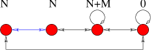
Figure 27: The $L^{131}$ theory with $N_{4}=0$. The blue line indicate the massive fields

with superpotential

$$W=X_{33}q_{32}q_{23}-\mu_{3}^{2}X_{33}-hq_{12}q_{23}q_{32}q_{21}+hm^{2}q_{12}q_{21}$$ (106)

with $m^{2}=\mu_{3}^{2}+\mu_{4}^{2}$. The adjoint field has a linear term and the quarks have a mass generally different from the deformation of the adjoint field. We take the ranks of the gauge groups as

$$N_{3}=N+M\qquad N_{2}=N_{3}=N\quad N_{4}=0$$ (107)

with $M>N$. With this choice we are guaranteed that the second node is infrared free. We consider the other groups less coupled.

Solving the equation of motion and expanding around the tree level minimum we have

$$q_{32}=\left(\begin{array}[]{c}\mu_{3}+\sigma_{1}\\ \phi_{1}\end{array}\right)\quad q_{23}\left(\begin{array}[]{c c}\mu_{3}+\sigma_{2}&\phi_{2}\end{array}\right)\quad X_{33}=\left(\begin{array}[]{c c}\sigma_{3}&\phi_{3}\\ \phi_{4}&\chi\end{array}\right)\quad q_{21}=\sigma_{4}\quad q_{12}=\sigma_{5}$$ (108)

where $\chi$ is a classical flat direction not associated to any broken symmetry. The case with $\mu_{4}=0$ (and hence $m^{2}=\mu_{3}^{2}$) is problematic since in this case the quarks $q_{12}$ and $q_{21}$ are potentially dangerous tree level flat directions.

Now, the non supersymmetric sector (the fields $\phi_{i}$) gives the usual O’Raifeartaigh like model of ISS which gives positive squared mass through 1 loop corrections to the pseudomoduli $\chi$. The fields $\phi_{i}$ get tree level masses except the Goldstone bosons as in the ISS model.

In the supersymmetric sector, the $\sigma_{1},\sigma_{2},\sigma_{3}$ fields are stabilized as in ISS. The fields $\sigma_{4}$ and $\sigma_{5}$ get non trivial squared mass $\sim|hm^{2}-h\mu^{2}|^{2}=|h\mu_{4}^{2}|^{2}$.

D.2 $L^{141}$

We analyze here a more complicated example, explained in section 3.2.1, that arises setting to zero a node in the $L^{141}$ quiver gauge theory. The resulting quiver is reported in figure 28

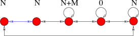
Figure 28: The $L^{141}$ theory with $N_{4}=0$. The blue line indicate the massive fields

and the superpotential is the following

$$W=hq_{12}q_{23}q_{32}q_{21}-\mu_{3}^{2}X_{33}-X_{33}q_{32}q_{23}+\mu_{5}^{2}X_{55}+X_{55}q_{51}q_{15}-hq_{51}q_{12}q_{21}q_{15}+hm^{2}q_{12}q_{21}$$ (109)

where all the adjoint fields receive a linear term. From the geometric description we know that

$$m^{2}=\mu_{3}^{2}+\mu_{4}^{2}-\mu_{5}^{2}$$ (110)

where $\mu_{4}^{2}$ is related to the node we have set to zero. Having set the ranks of the gauge group to be

$$N_{1}=N_{2}=N_{5}=N\qquad N_{3}=N+M\quad N_{4}=0$$ (111)

a rank condition mechanism is realized for the $X_{33}$ meson.

Solving the equation of motion and expanding around the tree level minimum we have

$$q_{23}=\left(\begin{array}[]{c}\mu_{3}+\sigma_{1}\\ \phi_{1}\end{array}\right)\quad q_{32}\left(\begin{array}[]{c c}\mu_{3}+\sigma_{2}&\phi_{2}\end{array}\right)\quad X_{33}=\left(\begin{array}[]{c c}\sigma_{3}&\phi_{3}\\ \phi_{4}&\chi\end{array}\right)$$ (117)

$$q_{12}=\sigma_{4}\quad q_{21}=\sigma_{5}\quad q_{51}=\mu_{5}+\sigma_{6}\quad q_{15}=\mu_{5}+\sigma_{7}\quad X_{55}=\sigma_{8}\,.$$ (118)

The non supersymmetric sector (the $\phi_{i}$ fields) is like the ISS model, and give raise to an O’Raifeartaigh model which stabilize at one loop the pseudomodulus at $\chi=0$.

The supersymmetric sector (the $\sigma_{i}$ fields) has the following superpotential at the relevant order for the mass matrix

$$W=\mu_{3}\sigma_{3}(\sigma_{1}+\sigma_{2})-h\mu_{4}^{2}\sigma_{4}\sigma_{5}-\mu_{5}\sigma_{8}(\sigma_{6}+\sigma_{7})\,.$$ (119)

The $\sigma_{1},\sigma_{2},\sigma_{3}$ fields behave exactly as in ISS: some of them acquire tree level positive mass. The massless ones are either Goldstone bosons either pseudomoduli. The latter are lifted by the $D$ term potential for the $U(N_{2})$ gauge group.

The $\sigma_{4},\sigma_{5}$ fields have tree level masses and this is due to the fact that we have turned on all the possible deformation for the geometry, i.e. $\mu_{4}\neq 0$. Otherwise they would be dangerous flat directions.

The $\sigma_{6},\sigma_{7},\sigma_{8}$ fields behave as the $\sigma_{1},\sigma_{2},\sigma_{3}$ sector. However we note that here the pseudomoduli arising in these fields are lifted by the $D$ terms of the $U(N_{5})$ gauge group, that we have considered less coupled than the gauge group $U(N_{2})$.

D.3 $L^{151}$

We study here the quiver gauge theory presented in section 3.2.2. The aim is to find the relevant aspects for the generalization to the $L^{1n1}$ theory. After setting to zero a node in the $L^{151}$ theory we obtain the quiver in figure 29

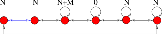
Figure 29: The $L^{151}$ theory with $N_{4}=0$. The blue line indicate the massive fields

with superpotential

$$W = X_{33}q_{23}q_{32}-hq_{12}q_{23}q_{32}q_{21}+hq_{61}q_{12}q_{21}q_{16}-X_{55}q_{56}q_{65}+X_{66}q_{65}q_{56}-X_{66}q_{61}q_{16}$$ (120)

$$-\mu_{3}^{2}X_{33}+\mu_{5}^{2}X_{55}+\mu_{6}^{2}X_{66}+hm^{2}q_{12}q_{21}\,.$$

The geometric description implies

$$m^{2}=\mu_{3}^{2}+\mu_{4}^{2}-\mu_{5}^{2}-\mu_{6}^{2}$$ (121)

where the parameter $\mu_{4}$ is related to the deformation for the node we have set to zero. The ranks of the groups are taken to be

$$N_{3}=N+M\qquad N_{1}=N_{2}=N_{5}=N_{6}=N\quad N_{4}=0\,.$$ (122)

Solving the equation of motion and expanding around the tree level minimum we have

$$q_{23}=\left(\begin{array}[]{c}\mu_{3}+\sigma_{1}\\ \phi_{1}\end{array}\right)\quad q_{32}\left(\begin{array}[]{c c}\mu_{3}+\sigma_{2}&\phi_{2}\end{array}\right)\quad X_{33}=\left(\begin{array}[]{c c}\sigma_{3}&\phi_{3}\\ \phi_{4}&\chi\end{array}\right)$$ (128)

$$q_{12}=\sigma_{4}\quad q_{21}=\sigma_{5}\quad q_{16}=\sqrt{\mu_{5}^{2}+\mu_{6}^{2}}+\sigma_{6}\quad q_{61}=\sqrt{\mu_{5}^{2}+\mu_{6}^{2}}+\sigma_{7}$$ (129)

$$X_{66}=\sigma_{8}\quad q_{65}=\mu_{5}+\sigma_{9}\quad q_{56}=\mu_{5}+\sigma_{10}\quad X_{55}=\sigma_{11}\,.$$ (130)

The non supersymmetric sector works as in the previous examples and stabilize the pseudomodulus $\chi$ at $\chi=0$. The supersymmetric sector (the $\sigma_{i}$) has, at the relevant order for the mass matrix, the following superpotential

$$W=\mu_{6}(\sigma_{11}-\sigma_{8})(\sigma_{9}+\sigma_{10})+\sqrt{\mu_{6}^{2}+\mu_{5}^{2}}\,\sigma_{8}(\sigma_{6}+\sigma_{7})-h\mu_{4}^{2}\sigma_{4}\sigma_{5}+\mu_{3}\sigma_{3}(\sigma_{1}+\sigma_{2})\,.$$ (131)

It can be analyzed as three separated sectors.

The first one is made by the fields $\sigma_{1},\sigma_{2},\sigma_{3}$ and behave exactly as in ISS. The second one is made by the fields $\sigma_{4},\sigma_{5}$. Here once again the parameter in the whole theory associated to the node set to zero ($\mu_{4}$) is crucial for the stability of the vacuum. In fact if $\mu_{4}=0$ the directions $\sigma_{4}$ and $\sigma_{5}$ would result massless at tree level.

The third sector is made by the other fields and it is stabilized at tree level taking into account the $D$ term contributions to the scalar potential for the gauge groups $U(N_{5})$ and $U(N_{6})$.

Another important fact to be stressed is that in this case we are not obliged to switch on the deformation $\mu_{6}$.

D.4 $L^{1n1}$

The analysis made in the last example can be extended to the gauge theory obtained from the $L^{1n1}$ quiver as explained in the text. The vacuum is chosen as a natural generalization of the previous examples, and the fluctuation superpotential has the same structure. The non supersymmetric sector is the same than in ISS. The supersymmetric sector is decoupled in three different parts as in the last subsection. The tree level flat directions are stabilized provided the deformation associated with the node set to zero and to the first and the last nodes are switched on.

Another requirement for stabilizing the flat directions in the $L^{1n1}$ theories with $n>3$ is to take into account the tree level $D$-term potential of some of the flavour groups. Note that for these nodes we need to consider also the $U(1)$ contribution to the $D$-term potential of the $U(n)$ groups. Otherwise, if the $U(1)$’s decouple, some flat directions due to the trace part of the fundamental fields can remain in the one loop spectrum. It would be interesting to explore their two loop behaviour.

D.5 Three nodes with two adjoint fields

We analyze the quiver gauge theory of figure 30

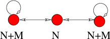
Figure 30: The quiver for the $L^{222}$ theory with a node set to zero

with superpotential

$$W=X_{11}q_{12}q_{21}-\mu_{1}^{2}X_{11}-hq_{12}q_{23}q_{32}q_{21}+hm_{1}^{2}q_{12}q_{21}+hm_{3}^{2}q_{32}q_{23}+X_{33}q_{32}q_{23}-\mu_{3}^{2}X_{33}\,.$$ (132)

We keep the more general situation arising from the geometries analyzed in the paper. That is the adjoint fields have linear terms and the quarks have masses generally different from the deformations of the adjoint field. The choice of the ranks for the gauge groups is

$$N_{1}=N_{3}=N+M\qquad N_{2}=N$$ (133)

with $2M>N$ and so we are guaranteed that the second node is infrared free. We consider this infrared free group as the most strongly coupled.

Solving the equation of motion and expanding around the tree level minimum we have

$$q_{12}=\left(\begin{array}[]{c}\mu_{1}+\sigma_{1}\\ \phi_{1}\end{array}\right)\quad q_{21}\left(\begin{array}[]{c c}\mu_{1}+\sigma_{2}&\phi_{2}\end{array}\right)\quad X_{11}=\left(\begin{array}[]{c c}h(\mu_{3}^{2}-m_{1}^{2})+\sigma_{3}&\phi_{3}\\ \phi_{4}&\chi_{1}\end{array}\right)$$ (139)

$$q_{32}=\left(\begin{array}[]{c}\mu_{3}+\sigma_{5}\\ \phi_{5}\end{array}\right)\quad q_{23}\left(\begin{array}[]{c c}\mu_{3}+\sigma_{6}&\phi_{6}\end{array}\right)\quad X_{33}=\left(\begin{array}[]{c c}h(\mu_{1}^{2}-m_{3}^{2})+\sigma_{7}&\phi_{7}\\ \phi_{8}&\chi_{2}\end{array}\right)$$ (145)

where $\chi_{1}$ and $\chi_{2}$ are the pseudomoduli. The superpotential for the supersymmetry breaking sector is

$$W = \chi_{1}\phi_{1}\phi_{2}-\mu_{1}^{2}\chi_{1}+\mu_{1}(\phi_{1}\phi_{4}+\phi_{2}\phi_{3})-h(\mu_{3}^{2}-m_{1}^{2})\phi_{1}\phi_{2}+$$ (146)

$$+ \chi_{2}\phi_{5}\phi_{6}-\mu_{3}^{2}\chi_{2}+\mu_{3}(\phi_{5}\phi_{8}+\phi_{6}\phi_{7})-h(\mu_{1}^{2}-m_{3}^{2})\phi_{5}\phi_{6}$$

and it consists in two O’Raifeartaigh like models after shifting the pseudomoduli as $\chi_{1}^{\prime}=\chi_{1}-h(\mu_{3}^{2}-m_{1}^{2})$ and $\chi_{2}^{\prime}=\chi_{2}-h(\mu_{1}^{2}-m_{3}^{2})$. Hence the pseudomoduli are stabilized at $\chi_{1}^{\prime}=\chi_{2}^{\prime}=0$ such that the non supersymmetric vacuum at quantum level is where the mesons $X_{11}$ and $X_{33}$ are proportional to the identity.

Appendix E Stability and UV completion

In this Appendix we discuss the issue of UV completion. A related problem concerns the unstable directions that can arise when we set some node to zero. The most natural UV completion to the IR theories analyzed in this paper seems to describe them as the last step of a duality cascade. If this is the case there could be potentially dangerous baryonic flat directions, due to the breaking of the baryonic symmetry. It occurs if we choose the baryonic branch after the confinement of some of the gauge groups. For supersymmetry, the Goldstone boson associated to the breaking of baryonic symmetry fits in a chiral supermultiplet containing another scalar particle that is not protected by any symmetry. This particle is a pseudogoldstone and signals a dangerous flat direction.

This scalar mode is decoupled at one loop and studying the stability of this direction remains an open problem. This was the case in [2, 4, 9]. A possible solution is the gauging of the baryonic symmetry. The resulting $D$-term potential lift these dangerous directions. Another possible way out, as noticed in [4], is to consider non canonical terms in the kahler potential. We comment on this problem and discuss it in a simple example, the $L^{444}$ theory.

We consider the quiver in figure 31 and we study its low energy dynamics.

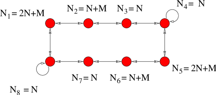
Figure 31: The $L^{444}$ theory which gives metastable vacua after the confinement of the nodes $N_{1}$ and $N_{5}$

Tuning the scales such that the first and the fifth node are the more strongly coupled gauge groups, we can describe the low energy with gauge singlets for these groups as

$$W= q_{23}q_{34}q_{43}q_{32}-q_{34}X_{44}q_{43}+M_{44}X_{44}-M_{46}M_{64}+q_{76}M_{66}q_{67}-\xi_{1}M_{66}+\xi_{1}X_{44}$$

$$- q_{67}q_{78}q_{87}q_{76}+q_{78}X_{88}q_{87}-M_{88}X_{88}+M_{82}M_{28}-q_{32}M_{22}q_{23}+\xi_{2}M_{22}-\xi_{2}X_{88}\,.$$

We observe that for the first and the fifth nodes the number of flavour coincides with the number of colors. Hence we have to impose the following quantum constraint on the moduli space

$$\det\left(\begin{array}[]{cc}M_{44}&M_{46}\\ M_{64}&M_{66}\end{array}\right)-b_{1}\tilde{b}_{1}-\Lambda_{1}^{4N+2M}=0$$ (149)

$$\det\left(\begin{array}[]{cc}M_{22}&M_{28}\\ M_{82}&M_{88}\end{array}\right)-b_{2}\tilde{b}_{2}-\Lambda_{2}^{4N+2M}=0\,.$$ (152)

Choosing the baryonic branch, we have $b_{i}\tilde{b}_{i}=\Lambda_{i}^{4N+2M}$, which breaks the baryonic symmetries. If we integrate out the massive mesons we obtain the low energy theory corresponding to set the nodes $N_{1}$ and $N_{5}$ to zero

$$W= q_{76}M_{66}q_{67}-\xi_{1}M_{66}-q_{67}q_{78}q_{87}q_{76}$$

$$- q_{32}M_{22}q_{23}+\xi_{2}M_{22}+q_{23}q_{34}q_{43}q_{32}\,.$$ (153)

This superpotential corresponds to two decoupled copies of theories obtained from $L^{131}$ setting to zero a node with an adjoint field, and where we set the two deformations to have the same value but opposite sign. This implies that there is not a mass term for the quarks. The two theories have metastable vacua, as shown in section 3.1.

As mentioned, the problem here is that the breaking of the global baryonic symmetry gives rise to a Goldstone boson and to a pseudoflat direction, which is not protected by any global symmetry. This direction does not receive any one loop contribution by the CW effective potential, and can get tachyonic at higher loops. The possible way out to this source of instability is that we are dealing with a compactified theory. This implies that the baryonic symmetry is gauged, and this gauging gives origin to a positive squared mass term for the pseudoflat direction.

References

- [1] K. Intriligator, N. Seiberg and D. Shih, JHEP 0604, 021 (2006) [arXiv:hep-th/0602239].
- [2] S. Franco and A. M. .. Uranga, JHEP 0606, 031 (2006) [arXiv:hep-th/0604136]. H. Ooguri and Y. Ookouchi, Nucl. Phys. B 755, 239 (2006) [arXiv:hep-th/0606061]. A. Amariti, L. Girardello and A. Mariotti, JHEP 0612, 058 (2006) [arXiv:hep-th/0608063]. M. Eto, K. Hashimoto and S. Terashima, JHEP 0703, 061 (2007) [arXiv:hep-th/0610042]. E. Dudas, C. Papineau and S. Pokorski, JHEP 0702, 028 (2007) [arXiv:hep-th/0610297]. L. Anguelova, R. Ricci and S. Thomas, Phys. Rev. D 77, 025036 (2008) [arXiv:hep-th/0702168]. S. Hirano, JHEP 0705, 064 (2007) [arXiv:hep-th/0703272]. K. Intriligator, N. Seiberg and D. Shih, JHEP 0707, 017 (2007) [arXiv:hep-th/0703281]. I. Garcia-Etxebarria, F. Saad and A. M. Uranga, JHEP 0705, 047 (2007) [arXiv:0704.0166 [hep-th]]. C. Angelantonj and E. Dudas, Phys. Lett. B 651, 239 (2007) [arXiv:0704.2553 [hep-th]]. H. Ooguri, Y. Ookouchi and C. S. Park, arXiv:0704.3613 [hep-th]. E. Dudas, J. Mourad and F. Nitti, JHEP 0708, 057 (2007) [arXiv:0706.1269 [hep-th]]. R. Essig, K. Sinha and G. Torroba, JHEP 0709, 032 (2007) [arXiv:0707.0007 [hep-th]]. H. Abe, T. Higaki and T. Kobayashi, Phys. Rev. D 76 (2007) 105003 [arXiv:0707.2671 [hep-th]]. R. Tatar and B. Wetenhall, Phys. Rev. D 76, 126011 (2007) [arXiv:0707.2712 [hep-th]]. H. Abe, T. Kobayashi and Y. Omura, JHEP 0711, 044 (2007) [arXiv:0708.3148 [hep-th]]. L. Anguelova and V. Calo, arXiv:0708.4159 [hep-th]. Y. Nakayama, M. Yamazaki and T. T. Yanagida, arXiv:0710.0001 [hep-th]. A. Giveon and D. Kutasov, arXiv:0710.0894 [hep-th]. J. Marsano, H. Ooguri, Y. Ookouchi and C. S. Park, arXiv:0712.3305 [hep-th]. C. Papineau, arXiv:0802.1861 [hep-th]. M. Arai, C. Montonen, N. Okada and S. Sasaki, JHEP 0803 (2008) 004 [arXiv:0712.4252 [hep-th]]. M. Arai, C. Montonen, N. Okada and S. Sasaki, Phys. Rev. D 76 (2007) 125009 [arXiv:0708.0668 [hep-th]].
- [3] S. Franco, I. Garcia-Etxebarria and A. M. Uranga, JHEP 0701, 085 (2007) [arXiv:hep-th/0607218]. H. Ooguri and Y. Ookouchi, Phys. Lett. B 641 (2006) 323 [arXiv:hep-th/0607183]. I. Bena, E. Gorbatov, S. Hellerman, N. Seiberg and D. Shih, JHEP 0611, 088 (2006) [arXiv:hep-th/0608157]. C. Ahn, Class. Quant. Grav. 24, 1359 (2007) [arXiv:hep-th/0608160]. R. Tatar and B. Wetenhall, JHEP 0702, 020 (2007) [arXiv:hep-th/0611303]. A. Giveon and D. Kutasov, Nucl. Phys. B 778, 129 (2007) [arXiv:hep-th/0703135]. A. Giveon and D. Kutasov, arXiv:0710.1833 [hep-th]. R. Tatar and B. Wetenhall, arXiv:0711.2534 [hep-th].
- [4] R. Argurio, M. Bertolini, S. Franco and S. Kachru, JHEP 0701, 083 (2007) [arXiv:hep-th/0610212].
- [5] M. Aganagic, C. Beem, J. Seo and C. Vafa, Nucl. Phys. B 789, 382 (2008) [arXiv:hep-th/0610249].
- [6] J. J. Heckman, J. Seo and C. Vafa, JHEP 0707, 073 (2007) [arXiv:hep-th/0702077].
- [7] R. Argurio, M. Bertolini, S. Franco and S. Kachru, JHEP 0706, 017 (2007) [arXiv:hep-th/0703236].
- [8] J. Marsano, K. Papadodimas and M. Shigemori, Nucl. Phys. B 789, 294 (2008) [arXiv:0705.0983 [hep-th]].
- [9] D. Malyshev, arXiv:0705.3281 [hep-th].
- [10] J. J. Heckman and C. Vafa, arXiv:0707.4011 [hep-th].
- [11] O. Aharony, S. Kachru and E. Silverstein, Phys. Rev. D 76, 126009 (2007) [arXiv:0708.0493 [hep-th]].
- [12] M. Aganagic, C. Beem and B. Freivogel, Nucl. Phys. B 795, 291 (2008) [arXiv:0708.0596 [hep-th]].
- [13] O. DeWolfe, S. Kachru and M. Mulligan, arXiv:0801.1520 [hep-th].
- [14] J. Marsano, K. Papadodimas and M. Shigemori, arXiv:0801.2154 [hep-th].
- [15] M. Buican, D. Malyshev and H. Verlinde, arXiv:0710.5519 [hep-th].
- [16] M. Aganagic, C. Beem and S. Kachru, arXiv:0709.4277 [hep-th].
- [17] K. Altmann, alg-geom/9403004v2
- [18] S. Franco, A. Hanany, F. Saad and A. M. Uranga, JHEP 0601, 011 (2006) [arXiv:hep-th/0505040].
- [19] M. R. Douglas, B. R. Greene and D. R. Morrison, Nucl. Phys. B 506 (1997) 84 [arXiv:hep-th/9704151].D. R. Morrison and M. R. Plesser, Adv. Theor. Math. Phys. 3, 1 (1999) [arXiv:hep-th/9810201].
- [20] I. R. Klebanov and M. J. Strassler, JHEP 0008 (2000) 052 [arXiv:hep-th/0007191].
- [21] S. Franco, A. Hanany and A. M. Uranga, JHEP 0509 (2005) 028 [arXiv:hep-th/0502113].
- [22] M. Cvetic, H. Lu, D. N. Page and C. N. Pope, Phys. Rev. Lett. 95, 071101 (2005) [arXiv:hep-th/0504225].
- [23] D. Martelli and J. Sparks, Phys. Lett. B 621 (2005) 208 [arXiv:hep-th/0505027].
- [24] S. Benvenuti and M. Kruczenski, JHEP 0604 (2006) 033 [arXiv:hep-th/0505206].
- [25] A. Butti, D. Forcella and A. Zaffaroni, JHEP 0509 (2005) 018 [arXiv:hep-th/0505220].
- [26] S. Franco, A. Hanany, D. Martelli, J. Sparks, D. Vegh and B. Wecht, JHEP 0601 (2006) 128 [arXiv:hep-th/0505211].
- [27] A. Amariti, L. Girardello and A. Mariotti, JHEP 0710, 017 (2007) [arXiv:0706.3151 [hep-th]].
- [28] I. Garcia-Etxebarria, F. Saad and A. M. Uranga, JHEP 0608 (2006) 069 [arXiv:hep-th/0605166].
- [29] M. Cvetic, H. Lu, D. N. Page and C. N. Pope, Phys. Rev. Lett. 95 (2005) 071101 [arXiv:hep-th/0504225]. D. Martelli and J. Sparks, Phys. Lett. B 621 (2005) 208 [arXiv:hep-th/0505027].
- [30] N. Seiberg, Nucl. Phys. B 435, 129 (1995) [arXiv:hep-th/9411149].
- [31] K. Intriligator and N. Seiberg, JHEP 0602 (2006) 031 [arXiv:hep-th/0512347].
- [32] A. Brini and D. Forcella, JHEP 0606, 050 (2006) [arXiv:hep-th/0603245].
- [33] M. Dine and W. Fischler, Phys. Lett. B 110, 227 (1982). M. Dine and W. Fischler, Nucl. Phys. B 204, 346 (1982). G. F. Giudice and R. Rattazzi, Phys. Rept. 322, 419 (1999) [arXiv:hep-ph/9801271].
- [34] M. Dine and J. Mason, Phys. Rev. D 77, 016005 (2008) [arXiv:hep-ph/0611312]. R. Kitano, H. Ooguri and Y. Ookouchi, Phys. Rev. D 75, 045022 (2007) [arXiv:hep-ph/0612139]. C. Csaki, Y. Shirman and J. Terning, JHEP 0705, 099 (2007) [arXiv:hep-ph/0612241]. O. Aharony and N. Seiberg, JHEP 0702, 054 (2007) [arXiv:hep-ph/0612308]. S. A. Abel and V. V. Khoze, arXiv:hep-ph/0701069. A. Amariti, L. Girardello and A. Mariotti, Fortsch. Phys. 55, 627 (2007) [arXiv:hep-th/0701121]. H. Murayama and Y. Nomura, Phys. Rev. D 75, 095011 (2007) [arXiv:hep-ph/0701231]. D. Shih, arXiv:hep-th/0703196. T. Kawano, H. Ooguri and Y. Ookouchi, Phys. Lett. B 652, 40 (2007) [arXiv:0704.1085 [hep-th]]. J. E. Kim, Phys. Lett. B 651, 407 (2007) [arXiv:0706.0293 [hep-ph]]. H. Y. Cho and J. C. Park, JHEP 0709, 122 (2007) [arXiv:0707.0716 [hep-ph]]. S. Abel, C. Durnford, J. Jaeckel and V. V. Khoze, arXiv:0707.2958 [hep-ph]. J. E. Kim, Phys. Lett. B 656, 207 (2007) [arXiv:0707.3292 [hep-ph]]. N. Haba and N. Maru, Phys. Rev. D 76 (2007) 115019 [arXiv:0709.2945 [hep-ph]]. N. Haba, arXiv:0802.1758 [hep-ph].
- [35] A. Hanany, C. P. Herzog and D. Vegh, JHEP 0607 (2006) 001 [arXiv:hep-th/0602041].
- [36] A. Butti, JHEP 0610 (2006) 080 [arXiv:hep-th/0603253].
- [37] A. Butti, D. Forcella and A. Zaffaroni, JHEP 0702 (2007) 081 [arXiv:hep-th/0607147].
- [38] S. Benvenuti, B. Feng, A. Hanany and Y. H. He, JHEP 0711 (2007) 050 [arXiv:hep-th/0608050].
- [39] A. Butti, D. Forcella and A. Zaffaroni, JHEP 0706 (2007) 069 [arXiv:hep-th/0611229].
- [40] S. Forste, Phys. Lett. B 642, 142 (2006) [arXiv:hep-th/0608036].