Effects of elastic heterogeneity and anisotropy on the morphology of self-assembled epitaxial quantum dots

Abstract

Epitaxial self-assembled quantum dots (SAQDs) are of both technological and fundamental interest, but their reliable manufacture still presents a technical challenge. To better understand the formation, morphology and ordering of epitaxial self-assembled quantum dots (SAQDs), it is essential to have an accurate model that can aid further experiments and predict the trends in SAQD formation. SAQDs form because of the destabilizing effect of elastic mismatch strain, but most analytic models and some numerical models of SAQD formation either assume an elastically homogeneous anisotropic film-substrate system or assume an elastically heterogeneous isotropic system. In this work, we perform the full film-substrate elastic calculation. Then we incorporate the elasticity calculation into a stochastic linear growth model. We find that using homogeneous elasticity can cause errors in the elastic energy density as large as $26\%$, and for typical modeling parameters lead to errors of about $11\%$ in the estimated value of average dot spacing. We also quantify the effect of elastic heterogeneity on the order estimates of SAQDs and confirm previous finding on the possibility of order enhancement by growing a film near the critical film height.

Copyright (2008) American Institute of Physics. This article may be downloaded for personal use only. Any other use requires prior permission of the author and the American Institute of Physics. The following article has been submitted to Journal of Applied Physics. After it is published, it will be found at (http://jap.aip.org).

I Introduction

Self-assembled quantum dots (SAQDs) function as artificial atoms embedded in a semiconductor matrix. Bimberg et al. (1999) As such, they are useful for a range of electronic and optoelectronic applications. Bayer et al. (2000); Akiyama et al. (2000); Viktorov and Mandel (2006); Kane (1998); Elzerman et al. (2004); Tanner et al. (2006); Li et al. (1996); Li and Xia (1997); Bimberg et al. (1999); Pchelyakov et al. (2000); Grundmann (2000); Petroff et al. (2001); Liu et al. (2001); Heinrichsdorff et al. (1997); Bimberg et al. (2002); Friesen et al. (2003); Cheng et al. (2003); Krebs et al. (2003); Sakaki (2003) For this reason, there has been a great deal of modeling work on their dynamic formation process. Spencer et al. (1991); Spencer et al. (1993a); Tekalign and Spencer (2004, 2007); Obayashi and Shintani (1998); Ross et al. (1998); Ozkan et al. (1999); Gao and Nix (1999); Holy et al. (1999); Ortiz et al. (1999); Zhang et al. (2003); Zhang and Bower (2001); Meixner et al. (2003); Liu et al. (2003a, b); Golovin et al. (2003); Friedman (2007a, b); Kumar and Friedman (2007); Ramasubramaniam and Shenoy (2005a, b); Niu et al. (2006) SAQDs are fabricated by depositing a semiconductor film on a lattice mismatched substrate with a smaller band gap, the most well-known examples being Ge_xSi_1-x deposited on Si and In_xGa_1-xAs deposited on GaAs. A good quantitative model of the SAQD formation can help in aiding understanding of the SAQD formation process and enable a sophisticated quantitative interpretation of experimental data, but more importantly, it can help move modeling from a descriptive mode to a predictive mode that could be used for process design optimization to aid in tasks such as the formation of new structures, control of morphology and enhancing order and reproducibility. Here, we improve upon previous spectral models of SAQD formation Spencer et al. (1991); Spencer et al. (1993a); Tekalign and Spencer (2004, 2007); Obayashi and Shintani (1998); Ozkan et al. (1999); Golovin et al. (2003); Friedman (2007a, b); Ramasubramaniam and Shenoy (2005a, b) by incorporating elastic anisotropy and elastic heterogeneity simultaneously. We also estimate the errors introduced by neglecting these effects.

Many reports in the literature make approximations such as assuming elastic isotropy, Spencer et al. (1991); Spencer et al. (1993b); Golovin et al. (2003); Kumar and Friedman (2007) elastic homogeneity of the film-substrate system Obayashi and Shintani (1998); Ozkan et al. (1999); Friedman (2007a, b); Ramasubramaniam and Shenoy (2005a, b) or making a thin film approximation. Tekalign and Spencer (2004, 2007) Here, we present a linear stochastic model of SAQD formation that incorporates anisotropic elasticity and the elastic heterogeneity of the film-substrate system. We investigate the SAQD spacing (a mean property) as well as the order of SAQD arrays that is determined by the fluctuations in the spacing and alignments (Fig. 1). Furthermore, we investigate the amount of error that previous approximations make (Table 1).

While there are other aspects of SAQD modeling that can be improved or incorporated, the presented work is an indispensable step in moving toward a more quantitatively accurate SAQD formation model. The elasticity portion of the calculation applies generally to different material systems, but other parts of the calculation such as surface energies and diffusional dynamics are specific to group IV elements that have four-fold symmetric SAQD formation dynamics such as Ge_xSi_1-x/Si,  Friedman (2007c, b, a) and not to II-VI systems or III-V systems such as In_xGa_1-xAs/GaAs.

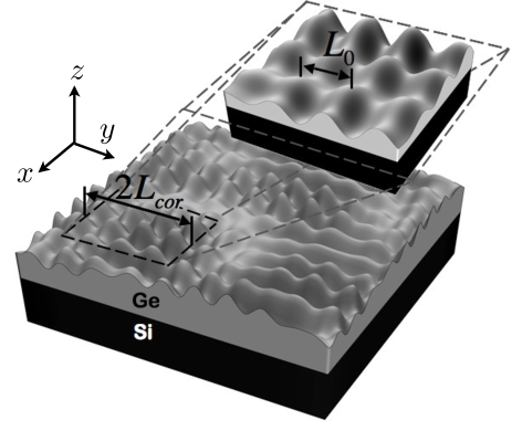
Figure 1: Initial formation of Ge/Si SAQDs (Sec. 1) with exaggerated height fluctuations for clarity. $L_{0}$ is mean dot spacing. $2L_{cor}$ is the length over which SAQDs appear periodic. (Sec. III).

SAQDs result from a transition from two-dimensional film growth to three-dimensional growth in strained epitaxial films. When a flat strained film is perturbed by a film height undulation, elastic energy is released. When the released energy is greater than the cost in surface and wetting energy, the perturbation grows. This phenomenon is known as the ATG (Asaro-Tiller-Grinfeld) instability. Asaro and Tiller (1972); Grinfeld (1986) Eventually the surface perturbations mature into 3D quantum dots. At a later stage the dots ripen, Liu et al. (2003a); Ross et al. (1998) although theoretically, they might form a uniform array under some circumstances. Wang et al. (2004); Golovin et al. (2003); Ross et al. (1998); Ortiz et al. (1999); Rastelli et al. (2005, 2006); Tu and Tersoff (2004) The interplay of the elastic energy, the surface energy and the wetting energy determines the energy landscape that drives SAQD formation, and the spectral modeling method used here yields a very transparent description of this interplay.

The spectral model can be used to define and estimate parameters characterizing SAQD formation such as the characteristic length and time scales, the mean SAQD spacing, the alignment of SAQDs in an array as well as the critical film height for SAQD formation.Spencer et al. (1991); Spencer et al. (1993b, a); Ozkan et al. (1999); Friedman (2007c, b) In the stochastic form, spectral modeling can also elucidate order and reproducibility of SAQD arrays. Friedman (2007a) In higher order versions of spectral models known as a multiscale-multitime analyses, they can even elucidate longer term evolution of SAQDs. Golovin et al. (2003) The clearly defined parameters from these models also inform finite element based models Zhang et al. (2003) and provide bench-marking for their performance.

Elasticity is the most well understood influence on SAQD formation. As such, making fewer approximations about elasticity will help investigations into other influences on SAQD formation that are more difficult to understand. For example, wetting energy is barely understood Suo and Zhang (1998); Zhang et al. (2003); Beck et al. (2004), and surface energy is generally treated as a constant, even though it almost certainly has strain and temperature dependence. It is also controversial as to whether surfaces should be treated as facets or not. Shenoy and Freund (2002); Tersoff et al. (2002)

While the importance of getting accurate estimates for a quantity as basic as the mean dot spacing is self-evident, the significance of SAQD order deserves further discussion. The ordering of SAQDs has been matter of concern in fostering the development of quantum dot based devices. Hong et al. (2006) There are two types of order, spatial and size. Spatial order is concerned with the uniformity of the spacings between the SAQDs and size order is concerned with the uniformity in the size of the SAQDs. The size and spacings of these self-assembled quantum dots are related, as dot volume is limited by the locally available material. Understanding what factors affect the order of SAQDs can guide experiments and simulation efforts and help in interpreting experimental and simulation results. Our enhanced elasticity calculation improves recent models of SAQD order. Friedman (2007c, b, a) We defer pattern fidelity in directed self-assembly to later work although some initial results have been previously reported. Zhao et al. (2006); Kumar and Friedman (2007)

Previous modeling work has focused on how elastic anisotropy and elastic heterogeneity affect SAQD formation, Friedman (2007b, a); Obayashi and Shintani (1998); Spencer et al. (1993b); Tekalign and Spencer (2004); Golovin et al. (2003); Liu et al. (2003c); Ozkan et al. (1999) but the two influences have been treated separately. The effect of elastic anisotropy has been studied in great detail. In Ref. Obayashi and Shintani (1998) it was shown that for heteroepitaxial system such as $\text{Si}_{1-x}\text{Ge}_{x}/\text{Si}$, the surface undulations are likely to grow in the $\langle 100\rangle$ directions. It was also shown that for anisotropic materials the growth rate of the amplitude of the surface fluctuations is maximum when the wavelength is $4/3$ the cutoff wavelength, similar to the isotropic approximation. However, in the presence of a strong wetting effect, this ratio increases to $2$. In the absence of misfit dislocations, the islands are aligned in the $\langle 100\rangle$ directions. However, experiments reveal that for films with thickness greater than the critical thickness for dislocation formation, in the later stages of island formation, the islands align along the $\langle 110\rangle$ directions due to formation of misfit dislocations. Ozkan et al. (1999) In Ref. Liu et al. (2003c) a numerical investigation was carried out to study the effect of anisotropic strength on the formation, alignment and average island spacing. More recent analytic studies on SAQD order Friedman (2007c, b, a) complement these numerical studies. The effect of elastic heterogeneity, however, has received more limited attention. In Ref. Spencer et al. (1993b) a linear stability analysis was performed that incorporated the elastic stiffness for both film and the substrate. One major conclusion was that elastically stiff substrate has stabilizing effects on the film that diminishes with increasing film thickness. In Ref. Tekalign and Spencer (2004) a nonlinear evolution equation was derived using a thin-film approximation. However, Refs. Spencer et al. (1993b) and Tekalign and Spencer (2004) approximate elasticity as isotropic.

Here, we treat elastic effects without approximations regarding isotropy, homogeneity or film thickness. We find various parameters that can be derived and estimated from spectral SAQD growth models, and we compare them with the results of the other more approximate models (Table 1). These parameters are $\mathcal{E}$, the elastic energy density coefficient (Figs. 2 and 3) $L_{E}$, the perturbation wavelength that is the most energetically unstable (Fig. 4), $L_{0}$, the perturbation wavelength that is kinetically most unstable and gives the mean dot spacing (Fig. 6), and ${n_{\text{cor}}}$ (Fig. 7), the number of dots in a row whose positions are well correlated. Each of these values is compared with the predictions of more approximate models, namely, the elastically anisotropic homogeneous approximation, the elastically anisotropic thin-film approximation, the elastically isotropic heterogeneous approximation, the elastically isotropic homogeneous approximation and the elastically isotropic thin-film approximation presented recently. Tekalign and Spencer (2007) For the order analysis, ${n_{\text{cor}}}$, comparisons are only made with the elastically anisotropic models as elastically isotropic models are not suitable for order predictions of periodic arrays. Friedman (2007c) Also, all of the reported estimates depend on the average film height ($\bar{H}$); thus for each comparison we present a calculation corresponding to a typical average film height of $\bar{H}=4.25\text{ ML}=1.2\text{ nm}$ in Table 1 with some additional values displayed in Figs. 3,  4 and 6–7. It is worth noting that all of these approximations correspond to various limits of our elasticity calculation. For example, the homogeneous anisotropic approximation is identical to the limit as the average film height ($\bar{H}$) becomes large. The anisotropic thin-film approximation corresponds to the limit as $\bar{H}\rightarrow 0$, and the various isotropic approximations can be obtained by using an isotropic elastic stiffness tensor by, for example, taking the Voigt or Reuss average of the actual elastic moduli. Finally, we give in-depth analysis throughout only for the anisotropic models.

We model the SAQD growth process with a stochastic surface diffusion model. We perform a linear analysis of the dynamics of the film evolution, which corresponds to small height fluctuations. Although such an analysis would only be valid for the onset of island formation, it determines the initial placement of SAQDs; thus determining the initial mean-spacing ($L_{0}$) and order (${n_{\text{cor}}}$). At later stages, the SAQDs either order or ripen Golovin et al. (2003); Liu et al. (2003c, b); Wang et al. (2004); Ross et al. (1998). The spacing and order established at the small fluctuation stage will influence the order at a later stage. This has also been verified through non-linear calculations in Ref. Friedman (2007a). Linear effects also set the length and the time scale for measuring the perturbations, Spencer et al. (1993b) and determine the arrangement of dots. Linearization offers a transparent way for analysis and is also a prerequisite for understanding more advanced non-linear models. The procedure for order analysis follows Refs. Friedman (2007b, c, a). Most models in literature are deterministic; however, the stochastic model is more realistic, as there is no rigorous physical explanation for the artificial initial random roughness in the deterministic models.

The rest of this article is organized as follows. We give details of the stochastic surface diffusion model in section II. In section III we discuss the order calculations using film height correlation functions. We present our conclusions in section IV.

II Model

The formation of SAQDs takes place through surface diffusion that is driven by a diffusion potential $\mu$ and contains thermal fluctuations, $\boldsymbol{\xi}(\mathbf{x},t)$. Friedman (2007a). $\mu$ is a non-local functional of the film height $H$ and a function of the horizontal position $\mathbf{x}=(x,y)$ (Fig. 1), so that $\mu\rightarrow\mu[H]\left(\mathbf{x}\right)$.

The normal velocity of the evolving film surface is

$$v_{n}=D\boldsymbol{\nabla}_{s}^{2}\mu+\boldsymbol{\nabla}_{s}\cdot\boldsymbol{\xi}(\mathbf{x},t),$$ (1)

where $\boldsymbol{\nabla}_{s}^{2}$ is the surface laplacian, $\boldsymbol{\nabla}_{s}\cdot$ is the surface divergence, and we omit explicit coordinate and time dependences for brevity. Here we consider the case of annealing of a film and therefore we omit a surface flux term in Eq. 1.

We linearize all quantities about the average film height $\bar{H}$,

$$H(\mathbf{x},t)=\bar{H}+h(\mathbf{x},t),$$ (2)

where the average film height $\bar{H}$ can be controlled by controlling the amount of deposited material and $h(\mathbf{x},t)$ represents the fluctuations about this average that cannot be experimentally controlled. In this procedure, the elastic contribution is non-local, so analysis is aided by working with Fourier components. Following Refs. Spencer et al. (1993b); Friedman (2007b) we use the Fourier transform convention, $f(\mathbf{x})=\int d^{2}\mathbf{x}\,e^{i{\mathbf{k}}\cdot\mathbf{x}}f_{{\mathbf{k}}}$ and $f_{{\mathbf{k}}}=\left(2\pi\right)^{-2}\int d^{2}{\mathbf{k}}\,e^{-i{\mathbf{k}}\cdot\mathbf{x}}f(\mathbf{x})$. Note that subscript ${\mathbf{k}}$ is used to indicate functions of wave vector ${\mathbf{k}}$ while $(\mathbf{x})$ is used to indicate dependence on the real-space coordinate. We proceed in two steps. First, we linearize the diffusion potential $\mu$. Then, we linearize the dynamic governing equations. Similar to Ref. Friedman (2007b), we keep terms only to linear order in $h(\mathbf{x},t)$.

Previously, the homogenous elasticity approximation was used to identify three related wavenumbers and wavelengths, Ozkan et al. (1999); Obayashi and Shintani (1998) the characteristic or cutoff wavenumber and wavelength $k_{c}$ and $L_{c}=2\pi/k_{c}$, the wavenumber and wavelength for maximum energy release, $k_{E}=\left(1/2\right)k_{c}$ and $L_{E}=2L_{c}$, Ozkan et al. (1999); Obayashi and Shintani (1998); Golovin et al. (2003) and the wavenumber and wavelength of the fastest growing mode was identified, $k_{0}$ and $L_{0}=2\pi/k_{0}$. Ozkan et al. (1999); Obayashi and Shintani (1998) In the absence of a wetting effect such as for thick films, $k_{0}=\left(3/4\right)k_{c}$ ($L_{0}=4/3L_{c}$), while for thin films where the wetting effect is strong, $k_{0}$ ranges from $k_{0}=k_{E}$ ($L_{0}=L_{E}$) at the critical film height to $k_{0}=(4/3)k_{E}$ ($L_{0}=(3/4)L_{E}$). Golovin et al. (2003); Friedman (2007c, b) In the less approximate formulation that is elastically heterogeneous and anisotropic, these relationships are not as simple. In the following analysis, we identify $k_{E}$ and $k_{0}$.

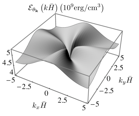
Figure 2: The elastic energy density prefactor as a function of the dimensionless vector ${\mathbf{k}}\bar{H}$ for Ge/Si at $600\,\text{K}$.

II.1 Energetics

The diffusion potential, $\mu$, consists of three parts, $\mu=\mu_{\text{elast.}}+\mu_{\text{surf}}+\mu_{\text{wet.}}$. Golovin et al. (2003, 2004); Tekalign and Spencer (2004); Zhang and Bower (2001); Friedman (2007c) The elastic energy part destabilizes the two-dimensional growth made, the surface energy term stabilizes the short wavelength (high-$k$) modes, and the wetting potential stabilizes all wavelengths. We proceed by calculating the Fourier transform of the diffusion potential, $\mu_{{\mathbf{k}}}$, to linear order in terms of the Fourier transform of the film height, $h_{{\mathbf{k}}}$.

II.1.1 Elastic anisotropy and heterogeneity

The elastic contribution to the diffusion potential is just the elastic energy density at the film surface, denoted $\omega\left(\mathbf{x}\right)$ times the atomic volume ($\mu_{\text{elast.}}=\Omega\omega(\mathbf{x})$). Freund and Suresh (2003) We proceed by calculating the Fourier transform of $\omega(\mathbf{x})$, $\omega_{{\mathbf{k}}}$ to linear order in surface height fluctuations, $h_{\mathbf{k}}$ while taking into account the effect of both elastic heterogeneity and elastic anisotropy.

The full calculation is described in the Appendix, and it results in an elastic energy density of the form

$$\omega_{{\mathbf{k}}}=-\mathcal{E}_{\theta_{{\mathbf{k}}}}(k\bar{H})kh_{{\mathbf{k}}},$$ (3)

where $\mathcal{E}_{\theta_{{\mathbf{k}}}}(k\bar{H})$ is the elastic energy density prefactor that depends on both wave vector direction $\theta_{{\mathbf{k}}}$ and dimensionless product $k\bar{H}$. Note that this form is equivalent to writing $\mathcal{E}\left({\mathbf{k}}\bar{H}\right)$ where ${\mathbf{k}}\bar{H}$ is a dimensionless vector quantity. This result should be contrasted with previous calculations. In the homogeneous isotropic approximation, the prefactor is a constant, and in the homogeneous anisotropic approximation, the prefactor depends only on the wavevector direction $\theta_{{\mathbf{k}}}$. Obayashi and Shintani (1998); Friedman (2007b)

We perform numerical calculations for [001]-oriented Ge/Si at $600\text{ K}$ to give a concrete example of the energy prefactor $\mathcal{E}_{\theta_{{\mathbf{k}}}}\left(k\bar{H}\right)$. The elastic stiffness tensor $c_{ijkl}$ is $4-\text{fold}$ symmetric for rotations about the [001] axis; thus $\mathcal{E}_{\theta_{{\mathbf{k}}}}\left(k\bar{H}\right)$ is also $4-\text{fold}$ symmetric. This symmetry manifests itself in the arrangement of SAQDs into a four-fold symmetric quasiperiodic lattice Obayashi and Shintani (1998); Gao and Nix (1999); Ozkan et al. (1999); Friedman (2007b). We use the following physical constants. The superscripts $f$ and $s$ differentiate between the elastic constants of the film and the substrate respectively. For Ge at $600\text{ K}$, the elastic constants are $c_{11}^{f}=11.99\times 10^{11}\,\text{dyn}/\text{cm}^{2}$, $c_{12}^{f}=4.01\times 10^{11}\,\text{dyn}/\text{cm}^{2}$ and $c_{44}^{f}=6.73\times 10^{11}\,\text{dyn}/\text{cm}^{2}$. Vorbyev (1996) For Si at $600\text{ K}$, $c_{11}^{s}=15.61\times 10^{11}\,\text{dyn}/\text{cm}^{2}$, $c_{12}^{s}=5.63\times 10^{11}\,\text{dyn}/\text{cm}^{2}$ and $c_{44}^{s}=7.82\times 10^{11}\,\text{dyn}/\text{cm}^{2}$. Vorbyev (1996) Using $a_{\text{Ge}}=0.5658\,\text{nm}$ and $a_{\text{Si}}=0.5431\,\text{nm}$, the mismatch strain is $\epsilon_{m}=0.0418$. Figure 2 shows a plot of the elastic energy prefactor, $\mathcal{E}_{\theta_{{\mathbf{k}}}}\left(k\bar{H}\right)$ against the dimensionless variables $k_{x}\bar{H}$ and $k_{y}\bar{H}$. Figure 3 shows $\mathcal{E}_{\theta_{{\mathbf{k}}}}\left(k\bar{H}\right)$ as a function of $k\bar{H}$ for three values of $\theta_{{\mathbf{k}}}$ along with a comparison to the discussed homogenous and isotropic approximations. In Figure 3, we can clearly see that as $k\bar{H}\rightarrow\infty$, the prefactor reaches its asymptotic values that also correspond to the homogeneous approximation.

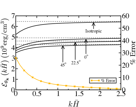
Figure 3: Elastic energy density prefactor $\mathcal{E}_{\theta_{{\mathbf{k}}}}$ for Ge/Si at $600\,\text{K}$ from isotropic approximations Spencer et al. (1993b) and anisotropic calculations for $\theta_{{\mathbf{k}}}=0^{\circ},22.5^{\circ}\,\text{and}\,45^{\circ}$. Asymptotically large $k\bar{H}$ limits corresponds to the anisotropic/isotropic homogeneous approximations and are shown as dotted lines ($\ldots$). Percent error in the values of $\mathcal{E}_{\theta_{{\mathbf{k}}}}$ for $\theta_{{\mathbf{k}}}=0^{\circ}$ is shown for the anisotropic homogeneous approximation.

Typical values for film height are $\bar{H}<20\,\text{ML}$, while typical relevant wavelengths are $30-40\text{ nm}$; thus, relevant values for $k\bar{H}$ are $<1$. In figure 3, we also plot the error due to the homogeneous anisotropic approximation for $\theta_{{\mathbf{k}}}=0^{\circ}$ and $0\leq k\bar{H}\leq 2.5$. For values of $k\bar{H}>2.5$ the error is significantly less (error $<1\%$). It should be noted that we focus primarily on the values at $\theta_{{\mathbf{k}}}=0^{\circ}$ because undulations are more likely to grow in the $\langle 100\rangle$ directions Obayashi and Shintani (1998); Ozkan et al. (1999); Friedman (2007b). At lower $k\bar{H}$ values ($k\bar{H}<0.4$) the error is higher ($>10\%$) with the upper bound being $26\%$. For example, for a periodic array of islands spaced at $L_{0}=49.06\,\text{nm}\,(k=2\pi/L_{0}=0.128\,\text{nm}^{-1})$ with average film height $\bar{H}=4.25\,\text{ML}=1.2\,\text{nm}$ so that $k\bar{H}=0.154$, the error in the calculation of elastic energy density is about $18\%$. We find that the anisotropic thin-film approximation does a bit better with an error of $-7\%$. We report these final values along with comparisons to other approximations in Table. 1. Such errors limit the accuracy of quantitative models, as this error propagates to calculations of the various characteristic wavenumbers (Secs. II.1.3 and II.2), mean dot spacing, rate of growth and critical film height.

Table 1: Comparison of presented model with various approximations. Our model uses heterogeneous anisotropic elasticity (Het. Anis.). Other models use homogeneous anisotropic elasticity (Hom. Anis.) Obayashi and Shintani (1998); Ozkan et al. (1999), anisotropic thin-film elasticity (Anis. Thin), heterogeneous isotropic elasticity (Het. Iso.) Spencer et al. (1993a), homogeneous isotropic elasticity (Hom. Iso.) and isotropic thin-film elasticity (Iso. Thin) Tekalign and Spencer (2007) All calculations use average film height $\bar{H}=4.25\text{ ML}$ and $\mathcal{E}_{0^{\circ}}(0.154)$ uses $k=2\pi/(49.06\text{nm})=0.128\text{ nm}^{-1}$. Values in parentheses indicate % error due to each approximation.

	Het. Anis.	Hom. Anis.	Anis. Thin	Het. Iso.	Hom. Iso.	Iso. Thin
		(% error)	(% error)	(% error)	(% error)	(% error)
$\mathcal{E}_{0^{\circ}}(0.154)$	$4.18$	$4.92$	$3.90$	$5.64$	$6.47$	$5.24$
($10^{9}$ erg/cm3)		$(+18\%)$	$(-7\%)$	$(+35\%)$	$(+56\%)$	$(+25\%)$
$L_{E}$ (nm)	$55.4$	$49.2$	$62.1$	$39.9$	$37.4$	$46.2$
		$(-11\%)$	$(+12\%)$	$(-28\%)$	$(-32.5\%)$	$(-17\%)$
$L_{0}$ (nm)	$49.1$	$43.7$	$55.1$	$35.4$	$33.2$	$41.0$
		$(-11\%)$	$(+12\%)$	$(-28\%)$	$(-32\%)$	$(-17\%)$
$n_{\text{cor.}}$	$2.71$	$2.07$	$2.62$	n/a	n/a	n/a
		$(+24\%)$	$(-3\%)$

II.1.2 Surface and Wetting energies

The other contributions to the SAQD formation energetics are the surface and wetting energies. Since our focus is on $4\text{--}$fold symmetric systems, the only anisotropic term is due to the elastic energy. Friedman (2007b) As in Ref. Friedman (2007b),

$$\mu_{\text{surf.,}{\mathbf{k}}}=\Omega(\gamma k^{2})h_{{\mathbf{k}}},$$ (4)

where $\gamma$ can be interpreted as the effective surface energy. Gao and Nix (1999); Friedman (2007b) The linearized wetting potential is

$$\mu_{\text{wet},{\mathbf{k}}}=\Omega\left(W^{\prime\prime}\right)h_{{\mathbf{k}}},$$ (5)

where $W^{\prime\prime}$ is the second derivative of the wetting potential with respect to the film height evaluated at the average film height $H=\bar{H}$. For the example here, we follow Ref. Zhang and Bower (2001) and take the wetting potential to be $W=B/H$, where $B$ is a material constant.

II.1.3 Energy cost function

Combining Eqs. 3, 4 and 5, we can write the linearized diffusion potential in Fourier space as

$$\mu_{{\mathbf{k}}}=f(k,\theta_{{\mathbf{k}}},\bar{H})h_{{\mathbf{k}}},$$ (6)

where $f(k,\theta_{{\mathbf{k}}},\bar{H})=\Omega\left[-k\mathcal{E}_{\theta_{{\mathbf{k}}}}(k\bar{H})+\gamma k^{2}+W^{\prime\prime}\right]$ is the energy cost per unit height for a periodic perturbation. The minima in the energy cost function lie along the $\left\langle 100\right\rangle$ directions ($\theta_{{\mathbf{k}}}=0^{\circ},\,90^{\circ},\,180^{\circ},\,270^{\circ}$) and occur at wavenumber $k_{E}$ so that the most energy is released when dots form at a period of $L_{E}=2\pi/k_{E}$. $L_{E}$ is a function of $\bar{H}$, a dependence that is due purely to the more precise elasticity calculation we present, and not, for example, a result of the wetting potential. For a concrete example, we use the estimated surface energy density $\gamma=1927\,\text{erg}/\text{cm}^{2}$ and the atomic volume $\Omega=2.27\times 10^{-23}\,\text{cm}^{3}$. Figure 4 shows $L_{E}$ as a function of $\bar{H}$ along with its values for the anisotropic homogenous and isotropic approximations. As $\bar{H}$ becomes large, $L_{E}$ approaches the anisotropic homogeneous approximation value that is independent of $\bar{H}$. For an average film height, $\bar{H}=4.25\,\text{ML}=1.2\,\text{nm}$, the error in $L_{E}$ from the homogeneous approximation is about $11\%$. We report results for all approximations in Table. 1.

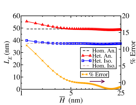
Figure 4: Characteristic wavelength $L_{E}$ as function of $\bar{H}$ for Ge/Si at $600\,\text{K}$ from isotropic and anisotropic calculations. Corresponding homogeneous approximations are shown as dashed lines. The percent error in is shown for the anisotropic homogeneous approximation.

The energy cost function is also useful for determining the critical film thickness for SAQD formation, or for modeling purposes it can be used to estimate the wetting potential that leads to an observed critical height. The critical height for SAQD formation in the Ge/Si film-substrate system is generally observed to be $4\text{--}6$ ML. Hegazy and Elsayed-Ali (2006) Here, we choose a critical film height of $4\,\text{ML}$ and follow the procedure from Ref. Zhang and Bower (2001). We assume a wetting potential of the form $W(H)=B/H$ and then find the coefficient $B$ that gives a critical film height, $H_{c}=4\,\text{ML}$, by setting the minimum value for the energy cost function to zero, $f_{\text{min}}=f(k_{E},0^{\circ},H_{c})=0$. Solving for $B$ is a simple procedure as $f$ is linear in $B$. We find that even the value of $B$ is sensitive to the anisotropic homogeneous and other approximations. At 4 ML, $B=1.61\times 10^{-6}\,\text{erg}/\text{cm}$ for the full theory, and $B=2.28\times 10^{-6}\,\text{erg}/\text{cm}$ for the anisotropic homogeneous approximation, about $42\%$ difference.

II.2 Dispersion Relation

The linearized evolution equation in Fourier space is given by Friedman (2007a)

$$\partial_{t}h_{{\mathbf{k}}}=\sigma_{{\mathbf{k}}}h_{{\mathbf{k}}}+\sqrt{2\Omega Dk_{b}T}\left[i{\mathbf{k}}\cdot\boldsymbol{\eta}_{{\mathbf{k}}}(t)\right],$$ (7)

where the second term is the Fourier transform of $\boldsymbol{\xi}(\mathbf{x},t)$ to linear order, $\langle\boldsymbol{\eta}_{{\mathbf{k}}}(t)\boldsymbol{\eta}_{{\mathbf{k}}^{\prime}}^{*}(t^{\prime})\rangle=(2\pi)^{-2}\tilde{I}\delta^{2}({\mathbf{k}}-{\mathbf{k}}^{\prime})\delta(t-t^{\prime})$ , Friedman (2007a) and

$$\sigma_{{\mathbf{k}}}=-Dk^{2}f(k,\theta_{{\mathbf{k}}},\bar{H})$$ (8)

is the generalized dispersion relation that gives the rate of growth (positive values) or decay (negative values) of each height Fourier component $h_{{\mathbf{k}}}$.

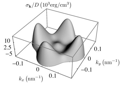
Figure 5: $\sigma_{{\mathbf{k}}}/D$ vs ${\mathbf{k}}$ for $\bar{H}=4.25\,\text{ML}$ for Ge/Si at $600\,\text{K}$.

Figure 5 shows the dispersion relation $\sigma_{\mathbf{k}}$ for $\bar{H}=4.25\,\text{ML}$. For the case shown in figure 5, $\sigma_{\mathbf{k}}$ has $4$ peaks along the $\langle 100\rangle$ directions at ${\mathbf{k}}_{0}=(0,\pm 0.128)\,\text{nm}^{-1}$ and $(\pm 0.128,0)\,\text{nm}^{-1}$. The four peaks indicate that the instability is maximum in the $\langle 100\rangle$ directions thus making them the likely directions for the alignment of SAQDs. This alignment is consistent with previous studies. Obayashi and Shintani (1998); Ozkan et al. (1999); Zhang et al. (2003); Friedman (2007b)

Similar to Ref. Friedman (2007b), we expand $\sigma_{{\mathbf{k}}}$ about its peak values to get

$$\sigma_{n}=\sigma_{0}-\frac{1}{2}\sigma_{\parallel}(k-k_{\parallel})^{2}-\frac{1}{2}\sigma_{\perp}k_{\perp}^{2},$$ (9)

where

$$\sigma_{\parallel}=-\left.\frac{\partial^{2}\sigma_{{\mathbf{k}}}}{\partial k^{2}}\right|_{\left[k_{0},(\theta_{0})_{n}\right]},\quad\sigma_{\perp}=-\frac{1}{k_{0}^{2}}\left.\frac{\partial^{2}\sigma_{{\mathbf{k}}}}{\partial\theta^{2}}\right|_{\left[k_{0},(\theta_{0})_{n}\right]},$$ (10)

$n$ corresponds to the number of peaks, $\theta_{0}$ is the orientation of ${\mathbf{k}}_{0}$, and $k_{\parallel}$ and $k_{\perp}$ are components parallel and perpendicular to ${\mathbf{k}}_{0}$. We discuss the dependence of $k_{0}$ and the mean dot spacing on film thickness next along with the discussion of SAQD array order.

III Order Analysis

The spatial order of SAQDs is best characterized by the mean geometric spacings, $L_{0}$, and alignments and by the degree of fluctuation about these means. The average alignment of SAQDs is $\left\langle 100\right\rangle$, and we characterize the range of order by, ${n_{\text{cor}}}$, the number of dots in a row whose positions are likely to be well correlated, meaning that they are likely to be both regularly spaced and well-aligned. In the following discussion we present calculations for different average film heights, and for each film height we calculate average dot spacing and the number of correlated dots when film height fluctuations reach atomic scale size. For the second part, for finding ${n_{\text{cor}}}$, we use the film height correlation function and associated correlation lengths which were derived previously. Friedman (2007c, b)

III.1 Average Dot Spacing

As done previously, Spencer et al. (1993a); Golovin et al. (2003); Friedman (2007c, b, a) we estimate the average initial spacing between dots to be $L_{0}=2\pi/k_{0}$. Figure 6 shows a plot of $L_{0}$ against $\bar{H}$ and compares it with the results for the anisotropic homogeneous and isotropic approximations. The error associated with the homogeneous approximation is also shown. We report values for $\bar{H}=1.2\text{ nm}$ in Table 1. For the example studied here (Ge/Si at $600\text{ K}$), the value of average spacing for anisotropic heterogeneous elasticity calculation varies between $32.8\,\text{nm}$ to $55.7\,\text{nm}$. Note that as $\bar{H}\rightarrow\infty$, $L_{0}$ reaches its asymptotic value, which is the same as the value from the anisotropic homogeneous approximation. Thus, the anisotropic homogeneous approximation is valid for thick films. Typically experiments correspond to values of $\bar{H}$ that are less than $20\,\text{ML}(4.25\,\text{nm})$.

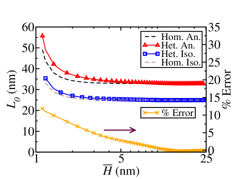
Figure 6: Average dot spacing $L_{0}$ as function of $\bar{H}$ for Ge/Si at $600\,\text{K}$ from isotropic and anisotropic calculations. Corresponding homogeneous approximations are shown as dashed lines. The percent error in is shown for the anisotropic homogeneous approximation.

III.2 Order Analysis Using Correlation Functions

The autocorrelation function and its Fourier transform, also known as the power spectrum, are very useful for characterizing dot order. Stangl et al. (2000); Springholz et al. (2001); Friedman (2007b) The autocorrelation function is defined as

$$C^{A}(\Delta\mathbf{x})=\int d^{2}\mathbf{x}\,h(\mathbf{x}+\Delta\mathbf{x})h(\mathbf{x}).$$

For an imperfectly periodic array of SAQDs the autocorrelation function decays away from the origin. The distance over which the autocorrelation function decays is known as the correlation length $L_{\text{cor}}$. The value $2L_{\text{cor}}$ represents the distance over which the SAQDs appear to be periodic meaning regularly spaced and well aligned.

The power spectrum is

$$C_{{\mathbf{k}}}^{A}=\left|h_{{\mathbf{k}}}\right|^{2}.$$

The power spectrum for a nearly periodic array of SAQDs will have peaks with finite width, $\Delta_{k}$. The spectrum peak width $\Delta_{k}$ is related to the correlation length $L_{\text{cor}}$ by $L_{\text{cor}}=1/\Delta_{k}$.

Each simulation or experiment corresponds to one particular realization with its own autocorrelation function; however, for sufficiently large simulation sizes, the fluctuations in $C^{A}\left(\Delta\mathbf{x}\right)$ are small, and the ensemble average of the autocorrelation functions can be predicted and provides a good estimate of individual autocorrelation functions and spectrum functions. Friedman (2007b) The ensemble average of the autocorrelation function is the correlation function $C(\Delta\mathbf{x})=\left\langle C^{A}(\Delta\mathbf{x})\right\rangle=\left\langle h(\Delta\mathbf{x})h(\mathbf{0})\right\rangle$. Similarly, the ensemble average spectrum function is $C_{{\mathbf{k}}}=\left\langle C_{{\mathbf{k}}}^{A}\right\rangle$, where $C_{{\mathbf{k}}}$ is also the Fourier transform of $C(\Delta\mathbf{x})$, and $C_{{\mathbf{k}}}$ is the coefficient in the covariance of the Fourier components $h_{{\mathbf{k}}}$; $\left\langle h_{{\mathbf{k}}}h_{{\mathbf{k}}^{\prime}}^{*}\right\rangle=C_{{\mathbf{k}}}\delta^{2}({\mathbf{k}}-{\mathbf{k}}^{\prime})$, where $\delta^{2}({\mathbf{k}}-{\mathbf{k}}^{\prime})$ is the two-dimensional Dirac Delta function.

The spectrum function can be solved using Eqs. 7, 9 and 10, Friedman (2007a)

$$C_{{\mathbf{k}}}\approx\frac{D\Omega k_{b}T}{(2\pi)^{2}\sigma_{0}}k^{2}e^{2\sigma_{0}t}\sum_{n=1}^{4}e^{-\frac{1}{2}L_{\parallel}^{2}(k_{\parallel}k_{0})^{2}-\frac{1}{2}L_{\perp}^{2}k_{\perp}^{2}},$$ (11)

where $L_{\parallel}=\sqrt{2\sigma_{\parallel}t}$ and $L_{\perp}=\sqrt{2\sigma_{\perp}t}$ are the correlation lengths. $L_{\parallel}$ gives about half the length over which the dot spacing is regular, while $L_{\perp}$ gives about half the length over which a row of dots is straight. Of the two correlation lengths, $L_{\perp}$ tends to be smaller and thus more limiting. Taking the inverse Fourier transform, the correlation function is

$$C(\mathbf{\Delta x})\approx\frac{D\Omega k_{b}Tk^{2}}{\pi\sigma_{0}L_{\parallel}L_{\perp}}e^{2\sigma_{0}t}\left[e^{-\frac{1}{2}(\Delta x^{2}/L_{\parallel}^{2}+\Delta y^{2}/L_{\perp}^{2})}\cos(k\Delta x)\right.\\ \left.+e^{-\frac{1}{2}(\Delta x^{2}/L_{\perp}^{2}+\Delta y^{2}/L_{\parallel}^{2})}\cos(k\Delta y)\right].$$ (12)

Figure 7 shows the number of correlated dots calculated as ${n_{\text{cor}}}=2L_{\perp}/L_{0}$ for the small fluctuation stage ($C(\mathbf{\Delta x}=\mathbf{0})=1\,\text{ML}^{2}$). Both error and number of correlated dots decline sharply for a small increment in film height above the critical film height. We find the error drops from $24\%$ at $\bar{H}=4.25\,\text{ML}$ to $3\%$ at $\bar{H}=4.95\,\text{ML}$. Note that with further increase in $\bar{H}$, the error fluctuates between $\pm 2\%$ before reaching $0\%$ for higher $\bar{H}$ values.

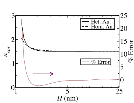
Figure 7: Number of correlated dots ${n_{\text{cor}}}$ for small height fluctuations Ge/Si at $600\,\text{K}$ for anisotropic heterogeneous and anisotropic homogeneous calculations. Also shown, error in ${n_{\text{cor}}}$ from anisotropic homogeneous approximation.

IV Conclusion

Most theoretical and many numerical models of SAQD growth approximate film-substrate systems as elastically homogeneous. We have examined the effect of elastic heterogeneity on SAQD mean spacing and the order estimates developed in Refs. Friedman (2007b) and Friedman (2007a). We have performed a linear analysis incorporating both elastic heterogeneity and elastic anisotropy. We quantify the effect of heterogeneity as percent error in the calculated values of elastic energy density, average spacing between the SAQDs and number of correlated dots based on homogeneous approximation. We show that the homogeneous approximation of the film-substrate system can lead to significant errors in the calculations for formation and ordering of SAQDs. For the case of Ge/Si system at $600\,\text{K}$ the upper bound for error in the calculated value of elastic energy density is found to be as large as $26\%$. The error declines as $\bar{H}$ increases. For a typical average film height, $\bar{H}=4.25\,\text{ML}$, we calculate an error of about $11\%$ in the estimation of average spacing between the SAQDs. Using a stochastic model, and the film height correlation functions, we find that the error in the estimated number of correlated dots declines quickly as $\bar{H}$ increases. The error in the estimated number of correlated dots drops from about $24\%$ at $\bar{H}=4.25\,\text{ML}$ to about $3\%$ at $\bar{H}=4.95\,\text{ML}$. For thinner films, the thin-film approximations can reduce this error, but error still remains as the thin-film approximation actually overestimates the effect of elastic heterogeneity. In general we find that the most error is due to using an isotropic approximation. For the isotropic heterogeneous approximation Spencer et al. (1993a) the error in mean dot spacing remains more or less constant at $34\%$ for values of $\bar{H}<20\,\text{ML}$. We did not report order predictions from isotropic models, as they are inappropriate for order and alignment estimates. Friedman (2007c)

The interplay between elastic strain, surface energy and surface diffusion can be quite complicated. Errors introduced by the elasticity portion of models can confound our ability to asses how well we model surface and wetting energy. Given the challenge of developing accurate models of surface and wetting energies, it is essential that the elasticity part of the calculation be correct. Here we have used a linear model that includes elastic anisotropy and heterogeneity. This is an important step in the development of a complete non-linear stochastic model required for a more comprehensive quantitative analysis, for example incorporating surface energy and diffusive anisotropy. We have demonstrated that one must incorporate both elastic anisotropy and elastic heterogeneity to avoid the introduction of significant errors in the calculation of the elastic energy density and mean dot spacing. This effect will have important consequences for single layer arrays grown on a flat [001] surface, but should also suggest the magnitude of errors introduced in modeling other SAQD morphologies such as multilayers and growth on patterned substrate.

Appendix: Elastic Energy Coefficient

The increase in elastic energy due to the addition of a small material volume at the surface is just the elastic energy density at the surface. Freund and Suresh (2003) We calculate the elastic energy density using perturbation theory following Ref. Friedman (2007b), but here we take elastic heterogeneity into account. This calculation was performed previously but only with the approximation of isotropic elasticity. Spencer et al. (1993b); Tekalign and Spencer (2004) Here we incorporate both elastic heterogeneity and elastic anisotropy to calculate the elastic energy density at the film surface.

We consider a flat film on a substrate. The lattice mismatch between the film and the substrate introduces a misfit strain $\epsilon_{m}$ in the film and leads to a uniform stress distribution in the film given by Freund and Suresh (2003); Friedman (2007b)

$$\tilde{\sigma}_{m}=\begin{bmatrix}\sigma_{m}&0&0\\ 0&\sigma_{m}&0\\ 0&0&0\end{bmatrix},$$ (13)

where $\sigma_{m}=M\epsilon_{m}$, and $M$ is the biaxial modulus,

$$M=\left[c_{11}^{f}+c_{12}^{f}-2(c_{12}^{f})^{2}/c_{11}^{f}\right],$$ (14)

where $c_{11}^{f}$ and $c_{12}^{f}$ are elastic constants for the film. We perturb the film surface so the film height fluctuates as

$$h(\mathbf{x})=h_{0}e^{ikx},$$ (15)

where the cartesian coordinate system is set up so that $z=0$ or the $x\text{--}y$ plane lies at the interface of the film-substrate system, and the $x-$direction is aligned along ${\mathbf{k}}$. Then, we calculate the elastic energy to first order in the perturbation amplitude, $h_{0}$. This calculation requires four steps. First we must find the surface normal vector $\mathbf{n}$ to first order in $h_{0}$. Then, we must find the admissible equilibrium eigenmodes for the elastic displacement that have the same periodicity as the height perturbation. Then we must find the eigenmode coefficients from the surface boundary conditions and internal matching conditions (compatibility and equilibrium). Finally, we find the elastic energy density at the free surface to first order in $h_{0}$. The first step is simple, to the first order in $h_{0}$ the normal to the surface of the film is given by

$$\mathbf{n}(\mathbf{x})=-ikh_{0}e^{ikx}\mathbf{e}_{x}+\mathbf{e}_{z}.$$ (16)

The remaining three steps follow.

We find the elastic deformation eigenmodes that have the same periodicity as the perturbation, and that satisfy internal equilibrium; working with the displacement field $\mathbf{u}$ automatically satisfies compatibility away from internal interfaces. We first construct the rank $4$ elastic stiffness tensor for both film and the substrate for an arbitrary passive rotation $\theta_{{\mathbf{k}}}$ in the $x\text{--}y$ plane so that ${\mathbf{k}}$ can lie along any direction in the plane.

$$c_{qrst}^{f}(\theta_{{\mathbf{k}}})=\sum_{i,j,k,l=1}^{3}R(\theta_{{\mathbf{k}}})_{qi}R(\theta_{{\mathbf{k}}})_{rj}R(\theta_{{\mathbf{k}}})_{sk}R(\theta_{{\mathbf{k}}})_{tl}c_{ijkl}^{f}$$ (17)

and

$$c_{qrst}^{s}(\theta_{{\mathbf{k}}})=\sum_{i,j,k,l=1}^{3}R(\theta_{{\mathbf{k}}})_{qi}R(\theta_{{\mathbf{k}}})_{rj}R(\theta_{{\mathbf{k}}})_{sk}R(\theta_{{\mathbf{k}}})_{tl}c_{ijkl}^{s},$$ (18)

where we are using the superscript $f$ and $s$ for the film and the substrate respectively and $R(\theta_{{\mathbf{k}}})$ is the passive rotation matrix by an angle $\theta_{{\mathbf{k}}}$ about the $z-$axis. To match boundary conditions in a later step, displacements must have the form

$$u_{l}^{f}(x,y,z) =U_{l}e^{k(ix+\kappa z)}$$ (19)

$$u_{l}^{s}(x,y,z) =V_{l}e^{k(ix+\zeta z)}.$$ (20)

where $\kappa$ and $\zeta$ are unknown eigenvalues. The stress tensors in the film and the substrate are

$$\sigma_{qr}^{f} =\sum_{s,t=1}^{3}c_{qrst}^{f}\frac{\partial u_{s}^{f}}{\partial x_{t}}+(\tilde{\sigma}_{m})_{qr}$$ (21)

$$\sigma_{qr}^{s} =\sum_{s,t=1}^{3}c_{qrst}^{s}\frac{\partial u_{s}^{s}}{\partial x_{t}}.$$ (22)

For the film, the elastic equilibrium equations are

$$\sum_{q,s,t=1}^{3}\frac{\partial}{\partial x_{q}}c_{qrst}^{f}(\theta_{{\mathbf{k}}})\frac{\partial}{\partial x_{s}}u_{t}^{f}=0;n=1\ldots 3$$ (23)

$$\left(\sum_{t=1}^{3}C_{rt}^{f}(\theta_{{\mathbf{k}}},\kappa)U_{t}\right)k^{2}e^{k(ix+\kappa z)}=0,$$ (24)

where

$$C_{rt}^{f}(\theta_{{\mathbf{k}}},\kappa)=\sum_{q,s=1}^{3}c_{qrst}^{f}(\theta_{{\mathbf{k}}})(i\delta_{q1}+\delta_{q3}\kappa)(i\delta_{s1}+\delta_{s3}\kappa).$$ (25)

To obtain non-trivial solutions, we set the determinant of $C_{rt}^{f}(\theta_{{\mathbf{k}}},\kappa)$ to zero. We thus obtain six eigenvalues of $\kappa$ denoted by $\kappa^{p}$ with $p=1\ldots 6$. Each value of $\kappa=\kappa^{p}$ is substituted back into $C_{rt}(\theta_{{\mathbf{k}}},\kappa)$, and Eq. 24 is solved to find the corresponding eigenvectors $U_{l}^{p}$. The displacement components for the film in terms of the unknown coefficients $A_{p}$ are thus

$$u_{l}^{f}=ih_{0}\epsilon_{m}\sum_{p=1}^{6}A_{p}U_{l}^{p}e^{k(ix+\kappa^{p}z)},$$ (26)

where we assume that the perturbing elastic field displacement components are proportional to $\epsilon_{m}$ and $h_{0}$, and we put the prefactor $i=\sqrt{-1}$ in for convenience. We use the same procedure to find the eigenvalues and eigenvectors for the substrate displacements $u_{l}^{s}$, where $C_{rt}^{s}(\theta_{{\mathbf{k}}},\zeta)$ has the same form as Eq. 25, but using the substrate elastic constants, $c_{qrst}^{s}$. Six eigenvalues, $\zeta^{p}$ are obtained; however, we assume that the substrate is a semi-infinite solid so the displacement field $u_{l}^{s}=0$ at $z=-\infty$. Thus, we only retain the three eigenvalues with $\text{Re}\left[\zeta^{p}\right]>0$ that satisfy this condition and discard the other three. We find the displacement components of the substrate,

$$u_{l}^{s}=ih_{0}\epsilon_{m}\sum_{p=1}^{3}B_{p}V_{l}^{p}e^{k(ix+\zeta^{p}z)},$$ (27)

where $V_{l}^{p}$ are the eigenvectors, and $B_{p}$ are the unknown coefficients.

We now find the nine unknown coefficients ($A_{p}$ and $B_{p}$) using the traction-free boundary condition at the surface, and the internal matching conditions at the film-substrate interface, namely equilibrium and compatibility. The traction on the surface of the film is

$$T_{r}=\sum_{q=1}^{3}\sigma_{qr}^{f}n_{q},$$ (28)

where $z=\bar{H}+h(\mathbf{x})$. Substituting Eq. 21 into Eq. (28), we get

$$T_{r} =\sum_{q,s,t=1}^{3}\left[c_{qrst}^{f}(\theta_{{\mathbf{k}}})\frac{\partial u_{s}}{\partial x_{t}}\right]n_{q}+(\tilde{\sigma}_{m})_{rq}n_{q}$$ (29)

$$=i\epsilon_{m}h_{0}\sum_{q,s,t=1}^{3}\sum_{p=1}^{6}c_{qrst}^{f}kA_{p}U_{s}^{p}(i\delta_{t1}\ldots$$

$$\ldots+\kappa^{p}\delta_{t3})e^{k(ix+\kappa^{p}z)}n_{q}+(\tilde{\sigma}_{m})_{rq}n_{q}.$$

Again, we substitute $z=\bar{H}+h(\mathbf{x})$, and we keep only terms up to first order in $h_{0}$ to get

$$\begin{split}T_{r}&=\left[\sum_{s=1}^{3}\sum_{p=1}^{6}\left(ic_{3rs1}^{f}(\theta_{{\mathbf{k}}})+\kappa^{p}c_{3rs3}^{f}(\theta_{{\mathbf{k}}})\right)A_{p}\right.\ldots\\ &\ldots\left.\times U_{s}^{p}e^{k\kappa^{p}\bar{H}}-M\delta_{r1}\right]ik\epsilon_{m}h_{0}e^{ikx}.\end{split}$$ (30)

Since the traction on the film surface must be zero, we have

$$\sum_{s=1}^{3}\sum_{p=1}^{6}\left(ic_{3rs1}^{f}(\theta_{{\mathbf{k}}})+\kappa^{p}c_{3rs3}^{f}(\theta_{{\mathbf{k}}})\right)A_{p}U_{s}^{p}e^{\kappa^{p}k\bar{H}}=M\delta_{r1}$$ (31)

giving three equations for $r=1\dots 3$.

The force balance at the internal film-substrate interface requires

$$\left.\sigma_{3r}^{f}=\sigma_{3r}^{s}\right|_{z=0}.$$ (32)

In terms of the unknown coefficients $A_{p}$ and $B_{p}$, we can write Eq. (32) as

$$\begin{split}\sum_{s=1}^{3}\sum_{p=1}^{6}\left(ic_{3rs1}^{f}+\kappa^{p}c_{3rs3}^{f}\right)A_{p}U_{s}^{p}&=\sum_{s=1}^{3}\sum_{p=1}^{3}\left(ic_{3rs1}^{s}\right.\ldots\\ \ldots&\left.+\zeta^{p}c_{3rs3}^{s}\right)B_{p}V_{s}^{p}\end{split}$$ (33)

for $r=1\dots 3$. For the compatibility between the film and the substrate at the interface, the displacements of the film and the substrate must be equal, so that

$$\left.u_{q}^{f}=u_{q}^{s}\right|_{z=0}.$$ (34)

In terms of the unknowns, the compatibility equation can be written as

$$\sum_{p=1}^{6}A_{p}U_{i}^{p}=\sum_{q=1}^{3}B_{q}V_{i}^{q}$$ (35)

giving three equations $i=1\dots 3$. We then calculate the nine coefficients, $A_{p}(\theta_{{\mathbf{k}}},k\bar{H})$ with $p=1\dots 6$ and $B_{q}(\theta_{{\mathbf{k}}},k\bar{H})$ with $q=1\dots 3$ using using Eqs. (31), (33) and (35).

Following Ref. Friedman (2007b), the we find the elastic energy at the film surface to first order in $h_{0}$ to be

$$U=U_{0}+M\epsilon_{m}\left.\left(\partial_{x_{1}}u_{1}^{f}+\partial_{x_{2}}u_{2}^{f}\right)\right|_{z=\bar{H}},$$ (36)

where $U_{0}$ is the energy of the unperturbed flat film, a constant. Using Eq. 26

$$U=U_{0}-\mathcal{E}_{\theta_{{\mathbf{k}}}}(k\bar{H})kh_{0}e^{ikx}\text{, where}$$ (37)

$$\mathcal{E}_{\theta_{{\mathbf{k}}}}(k\bar{H})=M\epsilon_{m}^{2}\sum_{p=1}^{6}A_{p}(\theta_{{\mathbf{k}}},k\bar{H})U_{1}^{p}(\theta_{{\mathbf{k}}}),$$ (38)

where we note that $A_{p}$ will depend on $\theta_{{\mathbf{k}}}$, $k$ and $\bar{H}$, and $U_{l}^{p}$ will depend on $\theta_{{\mathbf{k}}}$. By the principle of superposition, we can use the elastic energy coefficient $\mathcal{E}_{\theta_{{\mathbf{k}}}}\left(k\bar{H}\right)$ for sums of periodic perturbations as well.

References

- Bimberg et al. (1999) D. Bimberg, M. Grundmann, and N. N. Ledentsov, Quantum Dot Heterostructures (John Wiley & Sons, West Sussex, UK, 1999).
- Bayer et al. (2000) M. Bayer, O. Stern, P. Hawrylak, S. Fafard, and A. Forchel, Nature 405, 923 (2000).
- Akiyama et al. (2000) T. Akiyama, H. Kuwatsuka, T. Simoyama, Y. Nakata, K. Mukai, M. Sugawara, O. Wada, and H. Ishikawa, IEEE Photonics Technology Letters 12, 1301 (2000).
- Viktorov and Mandel (2006) E. A. Viktorov and P. Mandel, Applied Physics Letters 88, 201102 (2006).
- Kane (1998) B. E. Kane, Nature 393, 133 (1998).
- Elzerman et al. (2004) J. M. Elzerman, R. Hanson, L. H. W. van Beveren, B. Witkamp, L. M. K. Vandersypen, and L. P. Kouwenhoven, Nature 430, 431 (2004).
- Tanner et al. (2006) M. G. Tanner, D. G. Hasko, and D. A. Williams, Microelectronic Engineering 83, 1818 (2006).
- Li et al. (1996) S.-S. Li, J.-B. Xia, Z. L. Yuan, Z. Y. Xu, W. Ge, X. R. Wang, Y. Wang, J. Wang, and L. L. Chang, Phys. Rev. B 54, 11575 (1996).
- Li and Xia (1997) S.-S. Li and J.-B. Xia, Phys. Rev. B 55, 15434 (1997).
- Pchelyakov et al. (2000) O. P. Pchelyakov, Y. B. Bolkhovityanov, A. V. Dvurechenski, L. V. Sokolov, A. I. Nikiforov, A. I. Yakimov, and B. Voigtländer, Semiconductors 34, 122947 (2000), [doi:10.1134/1.1325416].
- Grundmann (2000) M. Grundmann, Physica E 5, 167 (2000), [doi:10.1016/S1386-9477(99)00041-7].
- Petroff et al. (2001) P. Petroff, A. Lorke, and A. Imamoglu, Phys. Today pp. 46–52 (2001), [doi:10.1063/1.1381102].
- Liu et al. (2001) H.-Y. Liu, B. Xu, Y.-Q. Wei, D. Ding, J.-J. Qian, Q. Han, J.-B. Liang, and Z.-G. Wang, Appl. Phys. Lett. 79, 2868 (2001).
- Heinrichsdorff et al. (1997) F. Heinrichsdorff, M. Mao, N. Kirstaedter, A. Krost, D. Bimberg, A. Kosogov, and P. Werner, Appl. Phys. Lett. 71, 22 (1997), [doi:10.1063/1.120556].
- Bimberg et al. (2002) D. Bimberg, N. Ledentsov, and J. Lott, MRS Bull. 27, 531 (2002).
- Friesen et al. (2003) M. Friesen, P. Rugheimer, D. E. Savage, M. G. Lagally, D. W. van der Weide, R. Joynt, and M. A. Eriksson, Phys. Rev. B 67, 121301 (R) (2003), [doi:10.1103/PhysRevB.67.121301].
- Cheng et al. (2003) Y.-C. Cheng, S. Yang, J.-N. Yang, L.-B. Chang, and L.-Z. Hsieh, Opt. Eng. 42, 11923 (2003), [doi:doi:10.1117/1.1525277].
- Krebs et al. (2003) R. Krebs, S. Deubert, J. Reithmaier, and A. Forchel, J. Cryst. Growth 251, 7427 (2003), [doi:10.1016/S0022-0248(02)02385-0].
- Sakaki (2003) H. Sakaki, J. Cryst. Growth 251, 9 (2003), [doi:10.1016/S0022-0248(03)00831-5].
- Spencer et al. (1991) B. J. Spencer, P. W. Voorhees, and S. H. Davis, Phys. Rev. Lett. 67, 3696 (1991), [doi:10.1103/PhysRevLett.67.3696].
- Spencer et al. (1993a) B. J. Spencer, P. W. Voorhees, and S. H. Davis, J. Appl. Phys. 73, 4955 (1993a), [doi: 10.1063/1.353815].
- Tekalign and Spencer (2004) W. T. Tekalign and B. J. Spencer, J. Appl. Phys. 96, 5505 (2004), [doi:10.1063/1.1766084].
- Tekalign and Spencer (2007) W. T. Tekalign and B. J. Spencer, J. Appl. Phys. 102, 073503 (2007).
- Obayashi and Shintani (1998) Y. Obayashi and K. Shintani, J. Appl. Phys. 84, 3141 (1998), [doi:10.1063/1.368468].
- Ross et al. (1998) F. M. Ross, J. Tersoff, and R. M. Tromp, Phys. Rev. Lett. 80, 984 (1998), [doi:10.1103/PhysRevLett.80.984].
- Ozkan et al. (1999) C. S. Ozkan, W. D. Nix, and H. J. Gao, J. Mater. Res. 14, 3247 (1999), [doi:10.1557/JMR.1999.043].
- Gao and Nix (1999) H. J. Gao and W. D. Nix, Ann. Rev. Mater. Sci. 29, 173 (1999), [doi:0.1146/annurev.matsci.29.1.173].
- Holy et al. (1999) V. Holy, G. Springholz, M. Pinczolits, and G. Bauer, Phys. Rev. Lett. 83, 356 (1999), [doi:10.1103/PhysRevLett.83.356].
- Ortiz et al. (1999) M. Ortiz, E. Repetto, and H. Si, Journal of the Mechanics and Physics of Solids 47, 697 (1999).
- Zhang et al. (2003) Y. Zhang, A. Bower, and P. Liu, Thin Solid Films 424, 9 (2003), [doi:10.1016/S0040-6090(02)00897-0].
- Zhang and Bower (2001) Y. W. Zhang and A. F. Bower, Appl. Phys. Lett. 78, 2706 (2001), [doi:10.1063/1.1354155].
- Meixner et al. (2003) M. Meixner, R. Kunert, and E. Scholl, Phys. Rev. B 67, 195301 (2003), [doi: 10.1103/PhysRevB.67.195301].
- Liu et al. (2003a) P. Liu, Y. W. Zhang, and C. Lu, Phys. Rev. B 67, 165414 (2003a), [doi: 10.1103/PhysRevB.67.165414].
- Liu et al. (2003b) P. Liu, Y. W. Zhang, and C. Lu, Phys. Rev. B 68, 035402 (2003b), [doi:10.1103/PhysRevB.68.035402].
- Golovin et al. (2003) A. A. Golovin, S. H. Davis, and P. W. Voorhees, Phys. Rev. E 68, 056203 (2003), [doi:10.1103/PhysRevE.68.056203].
- Friedman (2007a) L. H. Friedman, J. of Electron. Mater. 36, 1546 (2007a).
- Friedman (2007b) L. H. Friedman, J. of Nanophotonics 1, 013513 (2007b).
- Kumar and Friedman (2007) C. Kumar and L. H. Friedman, J. Appl. Phys. 101, 094903 (2007).
- Ramasubramaniam and Shenoy (2005a) A. Ramasubramaniam and V. B. Shenoy, J. Eng. Mater.-T. ASME 127, 434 (2005a), [doi:10.1115/1.1924559].
- Ramasubramaniam and Shenoy (2005b) A. Ramasubramaniam and V. B. Shenoy, J. Appl. Phys. 97, 114312 (2005b), [doi: 10.1063/1.1897837].
- Niu et al. (2006) X. Niu, R. Vardavas, R. E. Caflisch, and C. Ratsch, Phys. Rev. B 74, 193403 (2006), ISSN 1098-0121, [doi:10.1103/PhysRevB.74.193403.
- Spencer et al. (1993b) B. J. Spencer, S. H. Davis, and P. W. Voorhees, Phys. Rev. Lett. 47, 9760 (1993b), [doi: 10.1103/PhysRevB.47.9760].
- Friedman (2007c) L. H. Friedman, Phys. Rev. B 75, 193302 (2007c).
- Asaro and Tiller (1972) R. J. Asaro and W. A. Tiller, Met. Trans. 3, 1789 (1972).
- Grinfeld (1986) M. A. Grinfeld, Sov. Phys. Dokl. 31, 831 (1986).
- Wang et al. (2004) Y. U. Wang, Y. M. Jin, and A. G. Khachaturyan, Acta Mater. 52, 81 (2004), [doi:10.1016/j.actamat.2003.08.027].
- Rastelli et al. (2005) A. Rastelli, M. Stoffel, J. Tersoff, G. S. Kar, and O. G. Schmidt, Phys. Rev. Lett. 95, 026103 (2005), ISSN 0031-9007.
- Rastelli et al. (2006) A. Rastelli, M. Stoffel, U. Denker, T. Merdzhanova, and O. G. Schmidt, physica status solidi (a) 203, 3506 (2006).
- Tu and Tersoff (2004) Y. H. Tu and J. Tersoff, Phys. Rev. Lett. 93, 216101 (2004), ISSN 0031-9007, [doi:10.1103/PhysRevLett.93.216101.
- Suo and Zhang (1998) Z. Suo and Z. Zhang, Phys. Rev. B 58, 5116 (1998).
- Beck et al. (2004) M. J. Beck, A. van de Walle, and M. Asta, Phys. Rev. B 70, 205337 (2004), [doi:10.1103/PhysRevB.70.205337].
- Shenoy and Freund (2002) V. B. Shenoy and L. B. Freund, Journal of the Mechanics and Physics of Solids 50, 1817 (2002).
- Tersoff et al. (2002) J. Tersoff, B. J. Spencer, A. Rastelli, and H. von Känel, Phys. Rev. Lett. 89, 196104 (2002).
- Hong et al. (2006) S. U. Hong, J. S. Kim, J. H. Lee, H.-S. kwack, W.-S. Han, and D. K. Oh, J. Cryst. Growth 286, 18 (2006).
- Zhao et al. (2006) Z. M. Zhao, T. S. Yoon, W. Feng, B. Y. Li, J. H. Kim, J. Liu, O. Hulko, Y. H. Xie, H. M. Kim, K. B. Kim, et al., Thin Solid Films 508, 195 (2006), ISSN 0040-6090, [doi:10.1016/j.tsf.2005.08.407].
- Liu et al. (2003c) P. Liu, Y. W. Zhang, and C. Lu, Phys. Rev. B 68, 195314 (2003c), [doi:10.1103/PhysRevB.68.195314].
- Golovin et al. (2004) A. A. Golovin, M. S. Levine, T. V. Savina, and S. H. Davis, Phys. Rev. B 70, 235342 (2004), [doi:10.1103/PhysRevB.70.235342].
- Freund and Suresh (2003) L. B. Freund and S. Suresh, Thin Film Materials: Stress, Defect Formation and Surface Evolution (Cambridge University Press, Cambridge, UK, 2003), chap. 8.
- Vorbyev (1996) L. E. Vorbyev, Handbook Series On Semiconductor Parameters (World Scientific, Singapore, 1996), vol. 1.
- Hegazy and Elsayed-Ali (2006) M. S. Hegazy and H. E. Elsayed-Ali, J. Appl. Phys. 99, 054308 (2006).
- Stangl et al. (2000) J. Stangl, T. Roch, V. Holy, M. Pinczolits, G. Springholz, G. Bauer, I. Kegel, T. H. Metzger, J. Zhu, K. Brunner, et al., J. Vac. Sci. Technol. B 18 (2000).
- Springholz et al. (2001) G. Springholz, M. Pinczolits, V. Holy, S. Zerlauth, I. Vavra, and G. Bauer, Physica E 9, 149 (2001), [doi:10.1016/S1386-9477(00)00189-2.