Heat conduction and Fourier’s law in a class of many particle dispersing billiards

Abstract

We consider the motion of many confined billiard balls in interaction and discuss their transport and chaotic properties. In spite of the absence of mass transport, due to confinement, energy transport can take place through binary collisions between neighbouring particles. We explore the conditions under which relaxation to local equilibrium occurs on time scales much shorter than that of binary collisions, which characterize the transport of energy, and subsequent relaxation to local thermal equilibrium. Starting from the pseudo-Liouville equation for the time evolution of phase-space distributions, we derive a master equation which governs the energy exchange between the system constituents. We thus obtain analytical results relating the transport coefficient of thermal conductivity to the frequency of collision events and compute these quantities. We also provide estimates of the Lyapunov exponents and Kolmogorov-Sinai entropy under the assumption of scale separation. The validity of our results is confirmed by extensive numerical studies.

1 Introduction

Understanding the dynamical origin of the mechanisms which underly the phenomenology of heat conduction has remained one of the major open problems of statistical mechanics ever since Fourier’s seminal work [1]. Fourier himself actually warned his reader that the effects of heat conduction “make up a special range of phenomena which cannot be explained by the principles of motion and equilibrium,” thus seemingly rejecting the possibility of a fundamental level of description. Of course, with the subsequent developments of the molecular kinetic theory of heat, starting with the works of the founding-fathers of statistical mechanics, Boltzmann, Gibbs and Maxwell, and later with the definite triumph of atomism, thanks to Perrin’s 1908 measurement of the Avogadro number in relation to Einstein’s work on Brownian motion, Fourier’s earlier perception was soon discarded as it became clear that heat transport was indeed the effect of mechanical causes.

Yet, after well over a century of hard labor, the community is still actively hunting for a first principles based derivation of Fourier’s law, some authors going so far as to promise “a bottle of very good wine to anyone who provides [a satisfactory answer to this challenge]” [2]. Thus the challenge is, starting from the Hamiltonian time evolution of a system of interacting particles which models a fluid or a crystal, to derive the conditions under which the heat flux and temperature gradients are linearly related by the coefficient of heat conductivity. This is the embodiment of Fourier’s law.

As outlined in [2], it is necessary, in order to achieve this, that the model statistical properties be fully determined in terms of the local temperature, a notion which involves that of local thermalization. To visualize this, we imagine that the system is divided up into a large number of small volume elements, each large enough to contain a number of particles whose statistics is accurately described by the equilibrium statistics at the local temperature associated to the volume element under consideration. To establish this property, one must ensure that time scales separate, which implies that the volume elements settle to local thermal equilibrium on time scales much shorter than the ones which characterize the transport of heat at the macroscopic scale. Local thermal equilibrium therefore relies on very strong ergodic properties of the model.

The natural framework to apply this programme is that of chaotic billiards. Indeed non-interacting particle billiards, where individual tracers move and make specular collisions among a periodic array of fixed convex scatterers (the periodic Lorentz gases) are the only known Hamiltonian systems for which mass transport [3] and shear and bulk viscosities [4] have been established in a rigorous way. Here, rather than local thermal equilibrium, it is a relaxation to local equilibrium, occurring on the constant energy sheet of the individual tracer particles, which allows to model the mass transport by a random walk and yields an analytic estimate of the diffusion coefficient [5]. Arguably Lorentz gases, whether periodic or disordered, in or out of equilibrium, have played, over more than a century, a privileged and most important role in the development of transport and kinetic theories [6]. However, in the absence of interaction among the tracer particles, there is no mechanism for energy exchange and therefore no process of thermalization before heat is conducted. If, on the other hand, one adds some interaction between the tracers, say, as suggested in [2], by assigning them a size, the resulting system will typically have transport equations for the diffusion of both mass and energy. Though these systems may be conceptually simple, they are usually mathematically too difficult to handle with the appropriate level or rigor.

An example of billiard with interacting tracer particles is the modified Lorentz gas with rotating discs proposed by Mejía–Monasterio et al. [7]. This system exhibits normal transport with non-trivial coupled equations for heat and mass transport. Though this model has attracted much attention among mathematicians [8, 9, 10, 11, 12, 13], the rigorous proof of Fourier’s law for such a system of arbitrary size and number of tracers relies on assumptions which, though they are plausible, are themselves not resolved. Moreover the equations which govern the collisions and the discs rotations do not, as far as we know, derive from a Hamiltonian description.

Yet a remedy to such limitations with respect to the number of particles in interaction that a rigorous treatment will handle may have been just around the corner [14], and, this, within a Hamiltonian framework. Indeed in [15], Bunimovich et al. introduced a class of dispersing billiard tables with particles that are in geometric confinement –i. e. trapped within cells– but that can nevertheless interact among particles belonging to neighbouring cells. The authors proved ergodicity and strong chaotic properties of such systems with arbitrary number of particles.

More recently, the idea that energy transport can be modeled as a slow diffusion process resulting from the coupling of fast energy-conserving dynamics has led to proofs of central limit theorems in the context of models of random walks and coupled maps which describe the diffusion of energy in a strongly chaotic, fast changing environment [16, 17]. Although the extension of these results to symplectic coupled maps, let alone Hamiltonian flows, is not yet on the horizon, it is our belief that such systems as the dispersing billiard tables introduced in [15] will, if any, lend themselves to a fully rigorous treatment of heat transport within a Hamiltonian framework. As we announced in [18], the reason why we should be so hopeful is that the particles confinement has two important consequences : first, relaxation to local thermal equilibrium is preceded by a relaxation of individual particles to local equilibrium, which occurs at constant energy within each cell, and has strong ergodic properties that guarantee the rapid decay of statistical correlations; and, second, heat transport, unlike in the rotating discs model, can be controlled by the mere geometry of the billiard, which also controls the absence of mass transport. As of the first property, the relaxation to a local equilibrium before energy exchanges take place is characterized by a fast time scale, much faster than that of relaxation to local thermal equilibrium among neighbouring cells, which is itself much faster than the hydrodynamic relaxation scale. There is therefore a hierarchy of three separate time scales in this system, the first accounting for relaxation at the microscopic scale of individual cells, the second one at the mesoscopic scale of neighbouring cells, and the third one at the macroscopic scale of the whole system.

In this paper, we achieve two important milestones towards a complete first principles derivation of the transport properties of such models. Having defined the model, we establish the conditions for separation of time scales and relaxation to local equilibrium, identifying a critical geometry where binary collisions become impossible. Assuming relaxation to local equilibrium holds, we go on to considering the time evolution of phase-space densities and derive, from it, a master equation which governs the exchange of energy in the system [19], thus going from a microscopic scale description of the Liouville equation to the mesoscopic scale at which energy transport takes place. We regard this as the first milestone, namely identifying the conditions under which one can rigorously reduce the level of descrition from the deterministic dynamics at the microscopic level to a stochastic process described by a master equation at the mesoscopic level of energy exchanges.

This master equation is then used to compute the frequency of binary collisions and to derive Fourier’s law and the macroscopic heat equation, which results from the application of a small temperature gradient between neighbouring cells. This is our second milestone : an analytic formula for heat conductivity, exact for the stochastic system, and thus valid for the determinisitc system at the critical geometry limit. These results are then checked against numerical computations of these quantities, with outstanding agreement, and shown to extend beyond the critical geometry, with very good accuracy, to a wide range of parameter values.

We further characterize the chaotic properties of the model and offer arguments to account for the spectrum of Lyapunov exponents of the system, as well as the Kolmogorov-Sinai entropy, expressions which are exact at the critical geometry. Again, these results are very nicely confirmed by our numerical computations.

The paper is organized as follows. The models, which we coin lattice billiards, are introduced in section 2. Their main geometric properties are established, distinguishing transitions between insulating and conducting regimes under the tuning of a single parameter. The same parameter controls the time scales separation responsible for local equilibrium. Section 3 provides the derivation of the master equation which, under the assumption of local equilibrium, governs energy transport. The main observables are computed and their scaling properties discussed. In section 4 we review the properties of the model and assess the validity of the results of section 3 under the scope of our numerical computations. The chaotic properties of the models are discussed in section 5. We use simple theoretical arguments to predict some of these properties and compare them to numerical computations. Finally, conclusions are drawn in section 6.

2 Lattice billiards

To introduce our model, we start by considering the uniform motion of a point particle about a dispersing billiard table, $\mathcal{B}_{\rho}$, defined by the domain exterior to four overlapping discs of radii $\rho$, centered at the four corners of a square of sides $l$. The radius is thus restricted to the interval $l/2\leq\rho<l/\sqrt{2}$, where the lower bound is the overlap (or bounded horizon) condition, and the upper bound is reached when $\mathcal{B}_{\rho}$ is empty.

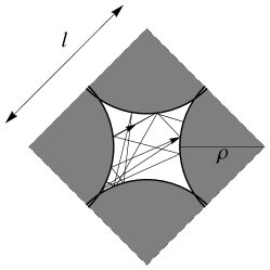
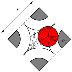
Figure 1: Two equivalent representations of a dispersing billiard table : (left) a point particle moves uniformly inside the domain $\mathcal{B}_{\rho}$ and performs specular collisions with its boundary; (right) a disc of radius $\rho_{\mathrm{m}}$ moves uniformly inside the domain $\mathcal{B}_{\rho}$ and performs specular collisions with fixed discs of radii $\rho_{\mathrm{f}}=\rho-\rho_{\mathrm{m}}$. The radius $\rho_{\mathrm{m}}$ is a free parameter which is allowed to take any value between 0 and $\rho$.

As illustrated in figure 1, the motion of a point particle in this environment is a limiting case of a class of equivalent dispersing billiards, whereby the point particle becomes a moving disc with radius $\rho_{\mathrm{m}}$, $0\leq\rho_{\mathrm{m}}\leq\rho$, and bounces off fixed discs of radii $\rho_{\mathrm{f}}=\rho-\rho_{\mathrm{m}}$. In all these cases, the motion of the center of the moving disc is equivalent to that of the point particle in $\mathcal{B}_{\rho}$. The border of the domain $\mathcal{B}_{\rho}$ constitutes the walls of the billiards.

In the absence of cusps (which occur at $\rho=l/2$), the ergodic and hyperbolic properties of these billiards are well established [20]. In particular, the long term statistics of the billiard map, which takes the particle from one collision event to the next, preserves the measure $\cos\phi\,\/\mathrm{d}\/r\,\/\mathrm{d}\/\phi$, where $\phi$ denotes the angle that the particle post-collisional velocity makes with respect to the normal vector to the boundary. A direct consequence of this invariance is a general formula which relates the mean free path, $\ell$, to the billiard table area, $|\mathcal{B}_{\rho}|$, and perimeter $|\partial\mathcal{B}_{\rho}|$, $\ell=\pi|\mathcal{B}_{\rho}|/|\partial\mathcal{B}_{\rho}|$.

The ratio between the speed of the particle, which we denote $\overline{v}$, and the mean free path gives the wall collision frequency, $\nu_{\mathrm{c}}=\overline{v}/\ell$, whose computation is shown in figure 2. With this quantity, one can relate the billiard map iterations to the time-continuous dynamics of the flow. In particular, the billiard map has two Lyapunov exponents, opposite in signs and equal in magnitudes, which, multiplied by the wall collision frequency, correspond to the two non-zero Lyapunov exponents of the flow (there are two additional zero exponents related to the direction of the flow and conservation of energy). The results of numerical computations of the positive one, denoted $\lambda_{+}$, are shown in figure 2 for different values of the parameters $\rho$.

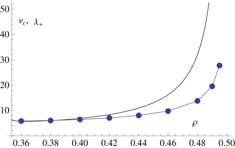
Figure 2: Collision frequency $\nu_{\mathrm{c}}$ (solid line) and numerical computation of the corresponding positive Lyapunov exponent of the flow (dots) of dispersing billiards such as shown in figure 1. Here we took $\overline{v}=1$ and the square side to be $l=1/\sqrt{2}$.

Thus let $Q(i,j)$ denote the rhombus of sides $l$ centered at point

$$(c_{ij},d_{ij})=\left\{\begin{array}[]{l@{\quad}l}(\sqrt{2}li,lj/\sqrt{2}),&j\ \mathrm{even},\\ (\sqrt{2}li+l/\sqrt{2},lj/\sqrt{2}),&j\ \mathrm{odd}.\\ \end{array}\right.$$ (1)

The rhombic billiard cell illustrated in figure 1 becomes a domain centered at point $(c_{ij},d_{ij})$, defined according to

$$\mathcal{B}_{\rho}(i,j)=\Big{\{}(x,y)\in Q(i,j)\Big{|}\delta[(x,y),(c_{ij}+p_{k},d_{ij}+q_{k})]\geq\rho,k=1,\dots,d\Big{\}},$$ (2)

where $\delta[.,.]$ denotes the usual Euclidean distance between two points, and $(p_{k},q_{k})=(\pm l/\sqrt{2},0),(0,\pm l/\sqrt{2})$ are the coordinates of the $d\equiv 4$ discs at the corners of the rhombus.

Now consider a number of copies $\{\mathcal{B}_{\rho}(i,j)\}_{i,j}$ which tessellate a two-dimensional domain. We define a lattice billiard as a collection of billiard cells

$$\mathcal{L}_{\rho,\rho_{\mathrm{m}}}(n_{1},n_{2}) \equiv \Big{\{}(x_{ij},y_{ij})\in\mathcal{B}_{\rho}(i,j)\Big{|}\delta[(x_{ij},y_{ij}),(x_{i^{\prime}j^{\prime}},y_{i^{\prime}j^{\prime}})]\geq 2\rho_{\mathrm{m}}$$ (3)

$$\forall\ 1\leq i,i^{\prime}\leq n_{1},1\leq j,j^{\prime}\leq n_{2},i\neq i^{\prime},j\neq j^{\prime}\Big{\}}.$$

Each individual cell of this billiard table possesses a single moving particle of radius $\rho_{\mathrm{m}}$, $0\leq\rho_{\mathrm{m}}\leq\rho$ and unit mass. All the moving particles are assumed to have independent initial coordinates within their respective cells, with the proviso that no overlap can occur between any pair of moving particles. The system energy, $E=Nk_{\mathrm{B}}T$ (with $N=n_{1}\times n_{2}$, the number of moving particles, $T$ the system temperature, and $k_{\mathrm{B}}$ Boltzmann’s constant) is constant and assumed to be initially randomly divided among the kinetic energies of the moving particles, $E=\sum_{i,j}\epsilon_{ij}$, $\epsilon_{ij}=mv_{ij}^{2}/2$, where $v_{ij}$ denotes the speed of particle $(i,j)$.

Energy exchanges occur when two moving particles located in neighbouring cells collide. Such events can take place provided the radii of the moving particles $\rho_{\mathrm{m}}$ is large enough compared to $\rho$. Indeed the value of the critical radius, below which binary collisions do not occur, is determined by half the separation between the corners of two neighbouring cells,

$$\rho_{\mathrm{c}}=\sqrt{\rho^{2}-\frac{l^{2}}{4}}.$$ (4)

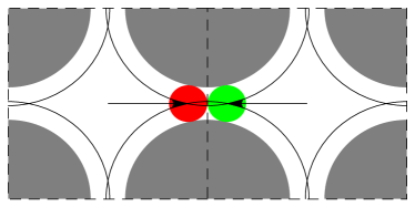
Figure 3: A binary collision event in the critical configuration where $\rho_{\mathrm{m}}=\rho_{\mathrm{c}}$ would occur only provided the colliding particles visit the corresponding corners of their cells simultaneously. The value of $\rho$ in this figure is the same as in figures 1 and 4.

For the sake of illustration, the unlikely occurrence of a binary collision event at the critical radius $\rho_{\mathrm{m}}=\rho_{\mathrm{c}}$ is shown in figure 3.

All the collisions are elastic and conserve energy, so that the dynamical system is Hamiltonian with $2N$ degrees of freedom. Its phase space of positions and velocities is $4N$-dimensional. Accordingly, the sensitivity to initial conditions of the dynamics is characterized by $4N$ Lyapunov exponents, $\{\lambda_{i}\}_{i=1}^{4N}$, obeying the pairing rule of symplectic systems, $\lambda_{4N-i+1}=-\lambda_{i}$, $i=1,\dots,2N$.

Collision events between two moving particles are referred to as binary collision events and will be distinguished from wall collision events, which occur between the moving particles and the walls of their respective confining cells. The occurrences of the former are characterized by a binary collision frequency, $\nu_{\mathrm{b}}$, and the latter by a wall collision frequency, $\nu_{\mathrm{w}}$. Both frequencies depend on the difference $\rho_{\mathrm{m}}-\rho_{\mathrm{c}}$, separating the moving particles radii from the critical radius, equation (4). By definition of $\rho_{\mathrm{c}}$, the binary collision frequency vanishes at $\rho_{\mathrm{m}}=\rho_{\mathrm{c}}$, $\nu_{\mathrm{b}}|_{\rho_{\mathrm{m}}=\rho_{\mathrm{c}}}=0$, and, correspondingly, the wall collision frequency at the critical radius is the collision frequency of the single-cell billiard, $\nu_{\mathrm{w}}|_{\rho_{\mathrm{m}}=\rho_{\mathrm{c}}}=\nu_{\mathrm{c}}$. We will assume from now, unless otherwise stated, that the system is globally isolated and apply periodic boundary conditions at the borders, thereby identifying $\mathcal{B}_{\rho}(i+kn_{1},j+ln_{2})$ with $\mathcal{B}_{\rho}(i,j)$ for any $k,l\in\mathbb{Z}$, $1\leq i\leq n_{1}$, $1\leq j\leq n_{2}$.

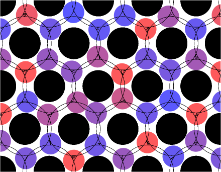
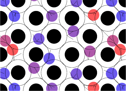
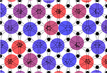
Figure 4: Examples of lattice billiards with triangular (top), rhombic (middle) and hexagonal (bottom) tilings. The coloured particles move among an array of fixed black discs. The radii of both fixed and mobile discs are chosen so that (i) every moving particle is geometrically confined to its own billiard cell (identified as the area delimited by the exterior intersection of the black circles around the fixed discs), but (ii) can nevertheless exchange energy with the moving particles in the neighbouring cells through binary collisions. The solid broken lines show the trajectories of the moving particles centers about their respective cells. The colours are coded according to the particles kinetic temperatures (from blue to red with increasing temperature).

Examples of such billiards are displayed in figure 4. Obviously the quincunx rhombic lattice structure, which is generated by the rhombic cells, is but one among different possible structures. Triangular, upright square, or hexagonal cells can be used as alternative periodic structures. One might also cover the plane with random or quasi-crystalline tessellations. The only relevant assumptions in what follows is that the moving particles must be confined to their (dispersing) billiard cells and that binary interactions between neighbouring cells can be turned on and off by tuning the system parameters.

The two important features of such lattice billiards is that (i) there is no mass transport across the billiard cells since the moving particles are confined to their respective cells, and (ii) energy transport can occur through binary collision events which take place when the particles of two neighbouring cells come into contact. In periodic structures such as the quincunx rhombic lattice, the possibility of such collisions is controlled by tuning the parameter $\rho_{\mathrm{m}}$ about the critical radius $\rho_{\mathrm{c}}$, keeping $\rho$ fixed.

We can therefore distinguish two separate regimes :

• Insulating billiard cells: $0\leq\rho_{\mathrm{m}}<\rho_{\mathrm{c}}$
  Absence of interaction between the moving discs. No transport process across the individual cells can happen;

• Conducting billiard cells: $\rho_{\mathrm{c}}<\rho_{\mathrm{m}}<\rho$
  Binary collision events are possible. Energy transport across the individual cells takes place.

The case $\rho_{\mathrm{m}}=\rho_{\mathrm{c}}$ is singular. We will refer to the critical geometry as the limit $\rho_{\mathrm{m}}\stackrel{{\scriptstyle>}}{{\to}}\rho_{\mathrm{c}}$.

In the insulating regime, there is no interaction among moving particles so that the billiard cells are decoupled. The moving particles are independent and their kinetic energies are individually conserved, resulting in $2N$ zero Lyapunov exponents. The equilibrium measure in turn has a product structure and phase-space distributions are locally uniform with respect to the particles positions and velocity directions. The $N$ positive Lyapunov exponents of the system are all equal to the positive Lyapunov exponent of the single-cell dispersing billiard, up to a factor corresponding to the particles speeds, $v_{ij}=\sqrt{2\epsilon_{ij}/m}$ : ${\lambda_{ij}}_{+}=v_{ij}\lambda_{+}$, where $\lambda_{+}$ is the Lyapunov exponent of the single-cell billiard measured per unit length.

When particles are allowed to interact, on the other hand, local energies are exchanged through collision events. Thus only the total energy is conserved in the conducting regime. The ergodicity of such systems of geometrically confined particles in interaction was proven by Bunimovich et al. [15]. The resulting dynamical system, whose equilibrium measure is the microcanonical one (taking into consideration that particles are otherwise uniformly distributed within their respective cells), enjoys the $K$-property. This implies ergodicity, mixing, and strong chaotic properties, including the positivity of the Kolmogorov-Sinai entropy. Two Lyapunov exponents are zero, one associated to the conservation of energy, the other to the direction of the flow. The $2(2N-1)$ remaining Lyapunov exponents form non-vanishing pairs of exponents with opposite signs, $\lambda_{1}>\dots>\lambda_{2N-1}>0$, $\lambda_{4N-i+1}=-\lambda_{i}$, $i=1,\dots,2N-1$.

The regime of interest to us is that corresponding to particles interacting rarely, which is to say, in analogy with a solid, that particles mostly vibrate inside their cells, ignorant of each other, and only seldom making collisions with their neighbours, thereby exchanging energy. As we turn on the interaction and let $\rho_{\mathrm{m}}\gtrsim\rho_{\mathrm{c}}$, binary collisions, though they can occur, will remain unlikely. This is to say that the binary collision frequency, $\nu_{\mathrm{b}}$, will, in this regime, remain small with respect to the wall collision frequency, $\nu_{\mathrm{w}}$, which in the absence of interaction and, in particular, at the critical geometry, we recall is equal to the wall collision frequency of the single-cell billiard, $\nu_{\mathrm{w}}|_{\rho_{\mathrm{m}}=\rho_{\mathrm{c}}}=\nu_{\mathrm{c}}$. When $\rho_{\mathrm{m}}\gtrsim\rho_{\mathrm{c}}$, we therefore expect $\nu_{\mathrm{w}}\gg\nu_{\mathrm{b}}$, as well as $\nu_{\mathrm{w}}\simeq\nu_{\mathrm{c}}$. In words : time scales separate. The consequence is that relaxation to local equilibrium –i. e. uniformization of the distribution of the particles positions and velocity directions at fixed speeds– occurs typically much faster than the energy exchange which drives the relaxation to the global equilibrium. This mechanism justifies resorting to kinetic theory in order to compute the transport properties of the model.

3 Kinetic theory

3.1 From Liouville’s equation to the master equation

The phase-space probability density is specified by the $N$-particles distribution function $p_{N}(\bi{r}_{1},\bi{v}_{1},\dots,\bi{r}_{N},\bi{v}_{N},t)$, where $\bi{r}_{a}$ and $\bi{v}_{a}$, $a=1,\dots,N$, denote the $a$th particle position and velocity vectors. The index $a$ stands for the label $(i,j)$ of the cells defined by equation (2). For our system, as is customary for hard sphere dynamics, this distribution satisfies a pseudo-Liouville equation [21], which is well defined despite the singularity of the hard-core interactions. This equation, which describes the time evolution of $p_{N}$ is composed of three types of terms: (i) the advection terms, which account for the displacement of the moving particles within their respective billiard cells; (ii) the wall collision terms, which account for the wall collision events, between the moving particles and the $d$ fixed scattering discs which form the cells walls; and (iii) the binary collision terms, which account for binary collision events, between moving particles belonging to neighbouring billiard cells :

$$\partial_{t}p_{N}=\sum_{a=1}^{N}\left[-\bi{v}_{a}\cdot\partial_{\bi{r}_{a}}+\sum_{k=1}^{d}K^{(a,k)}\right]p_{N}+\frac{1}{2}\sum_{a,b=1}^{N}B^{(a,b)}p_{N}.$$ (5)

Each wall collision term involves a single moving particle with index $a$ and one of the $d$ fixed discs in the corresponding cell, with index $k$ and position $\bi{R}_{k}$. Let $\bi{r}_{ak}=\bi{r}_{a}-\bi{R}_{k}$ denote their relative position. Following [22], we have

$$K^{(a,k)}p_{N}(\dots,\bi{r}_{a},\bi{v}_{a},\dots)=$$ (6)

$$\rho\int_{\hat{\bi{e}}\cdot\bi{v}_{a}>0}\/\mathrm{d}\/\hat{\bi{e}}(\hat{\bi{e}}\cdot\bi{v}_{a})\Big{[}\delta(\bi{r}_{ak}-\rho\hat{\bi{e}})p_{N}\big{(}\dots,\bi{r}_{a},\bi{v}_{a}-2\hat{\bi{e}}(\hat{\bi{e}}\cdot\bi{v}_{a}),\dots\big{)}$$

$$\hskip 99.58464pt-\delta(\bi{r}_{ak}-\rho\hat{\bi{e}})p_{N}\big{(}\dots,\bi{r}_{a},\bi{v}_{a},\dots\big{)}\Big{]},$$

where $\hat{\bi{e}}$ denotes the normal unit vector to the fixed disc $k$ in the cell of particle $a$.

Likewise the binary collision operator, written in terms of the relative positions $\bi{r}_{ab}$ and velocities $\bi{v}_{ab}$ of particles $a$ and $b$, and the unit vector $\hat{\bi{e}}_{ab}$ that connects them, is

$$B^{(a,b)}p_{N}(\dots,\bi{r}_{a},\bi{v}_{a},\dots,\bi{r}_{b},\bi{v}_{b},\dots)=$$ (7)

$$2\rho_{\mathrm{m}}\int_{\hat{\bi{e}}_{ab}\cdot\bi{v}_{ab}>0}\/\mathrm{d}\/\hat{\bi{e}}_{ab}(\hat{\bi{e}}_{ab}\cdot\bi{v}_{ab})\Big{[}\delta(\bi{r}_{ab}-2\rho_{\mathrm{m}}\hat{\bi{e}}_{ab})$$

$$\times p_{N}\big{(}\dots,\bi{r}_{a},\bi{v}_{a}-\hat{\bi{e}}_{ab}(\hat{\bi{e}}_{ab}\cdot\bi{v}_{ab}),\dots,\bi{r}_{b},\bi{v}_{b}+\hat{\bi{e}}_{ab}(\hat{\bi{e}}_{ab}\cdot\bi{v}_{ab}),\dots\big{)}$$

$$\hskip 99.58464pt-\delta(\bi{r}_{ab}+2\rho_{\mathrm{m}}\hat{\bi{e}}_{ab})p_{N}\big{(}\dots,\bi{r}_{a},\bi{v}_{a},\dots,\bi{r}_{b},\bi{v}_{b},\dots\big{)}\Big{]}.$$

We notice that only the terms $B^{(a,b)}$ corresponding to first neighbours are non-vanishing and contribute to the double sum on the RHS of equation (5).

Provided we have a separation of time scales between wall and binary collisions, the advection and wall collision terms on the RHS of equation (5) will typically dominate the dynamics on the short time $\sim 1/\nu_{\mathrm{w}}$, which follows every binary collision event, thus ensuring, thanks to the mixing within individual billiard cells, the relaxation of the phase-space distribution $p_{N}$ to local equilibrium well before the occurrence of the next binary event, whose time scale is $\sim 1/\nu_{\mathrm{b}}$. In other words, $p_{N}(\bi{r}_{1},\bi{v}_{1},\dots,\bi{r}_{N},\bi{v}_{N},t)$ quickly relaxes to a locally uniform distribution, which depends only on the local energies, justifying the introduction of

$$P^{(\mathrm{leq})}_{N}(\epsilon_{1},\dots,\epsilon_{N},t)\equiv\int\prod_{a=1}^{N}\/\mathrm{d}\/\bi{r}_{a}\/\mathrm{d}\/\bi{v}_{a}p_{N}(\bi{r}_{1},\bi{v}_{1},\dots,\bi{r}_{N},\bi{v}_{N},t)\prod_{a=1}^{N}\delta(\epsilon_{a}-mv_{a}^{2}/2),$$ (8)

where $v_{a}\equiv|\bi{v}_{a}|$. On the time scale of binary collision events, this distribution subsequently relaxes to the global microcanonical equilibrium distribution. This process accounts for the transport of energy, and can be characterized by the master equation [19]

$$\partial_{t}P^{(\mathrm{leq})}_{N}(\epsilon_{1},\dots,\epsilon_{N},t)=\frac{1}{2}\sum_{a,b=1}^{N}\int\/\mathrm{d}\/\eta$$

$$\hbox to0.0pt{\hss${}\times{}$}\Big{[}W(\epsilon_{a}+\eta,\epsilon_{b}-\eta|\epsilon_{a},\epsilon_{b})P^{(\mathrm{leq})}_{N}(\dots,\epsilon_{a}+\eta,\dots,\epsilon_{b}-\eta,\dots,t)$$

$$-W(\epsilon_{a},\epsilon_{b}|\epsilon_{a}-\eta,\epsilon_{b}+\eta)P^{(\mathrm{leq})}_{N}(\dots,\epsilon_{a},\dots,\epsilon_{b},\dots,t)\Big{]},$$ (9)

where $W(\epsilon_{a},\epsilon_{b}|\epsilon_{a}-\eta,\epsilon_{b}+\eta)$ denotes the probability that an energy $\eta$ be transferred from particle $a$ to particle $b$ as the result of a binary collision event between them. This equation is a closure for the local equilibrium distribution $P^{(\mathrm{leq})}_{N}$, obtained from equation (5) under the assumption that $\nu_{\mathrm{w}}\gg\nu_{\mathrm{b}}$. The first two terms on the RHS of equation (5) are eliminated because they leave invariant the local distribution $\prod_{a=1}^{N}\delta(\epsilon_{a}-mv_{a}^{2}/2)$. There remain the contributions (7) from the binary collisions, which, under the assumption that the local distibutions are uniform with respect to the positions and velocity directions, yield the following expression of $W$ :

$$W(\epsilon_{a},\epsilon_{b}|\epsilon_{a}-\eta,\epsilon_{b}+\eta)=\frac{2\rho_{\mathrm{m}}m^{2}}{(2\pi)^{2}|\mathcal{L}_{\rho,\rho_{\mathrm{m}}}(2)|}\int\/\mathrm{d}\/\phi\/\mathrm{d}\/\bi{R}\int_{\hat{\bi{e}}_{ab}\cdot\bi{v}_{ab}>0}\/\mathrm{d}\/\bi{v}_{a}\/\mathrm{d}\/\bi{v}_{b}$$ (10)

$$\hbox to0.0pt{\hss${}\times{}$}\hat{\bi{e}}_{ab}\cdot\bi{v}_{ab}\ \delta\left(\epsilon_{a}-\frac{m}{2}v_{a}^{2}\right)\delta\left(\epsilon_{b}-\frac{m}{2}v_{b}^{2}\right)\delta\left(\eta-\frac{m}{2}[(\hat{\bi{e}}_{ab}\cdot\bi{v}_{a})^{2}-(\hat{\bi{e}}_{ab}\cdot\bi{v}_{b})^{2}]\right),$$

where the first integration is performed over the positions of the center of mass, $\bi{R}\equiv(\bi{r}_{a}+\bi{r}_{b})/2$, between the two particles $a$ and $b$, given that they are in contact and both located in their respective cells, and over the angle $\phi$ of the unit vector connecting $a$ and $b$, $\hat{\bi{e}}_{ab}=(\cos\phi,\sin\phi)$. The normalizing factor $|\mathcal{L}_{\rho,\rho_{\mathrm{m}}}(2)|$ denotes the $4$-volume of the billiard corresponding to two neighbouring cells $a$ and $b$, which, with the assumption that $\rho_{\mathrm{m}}\gtrsim\rho_{\mathrm{c}}$, can be approximated by $|\mathcal{L}_{\rho,\rho_{\mathrm{m}}}(2)|\simeq|\mathcal{B}_{\rho}|^{2}$. This substitution amounts to neglecting the overlap between the two particles; see equation (23) for a refinement of that approximation. We point out that the position and velocity integrations in equation (10) can be formally decoupled; in this way, we can prove that the transition rate $W$ is given in terms of Jacobian elliptic functions, see A.

3.2 Geometric factor

As we show in A, an important property of the master equation (9) is that the factor which accounts for the geometry of collision events factorizes from the part of the kernel that accounts for energy exchanges. Therefore, as $\rho_{\mathrm{m}}\to\rho_{\mathrm{c}}$, the critical value of the radius at which binary collision events become impossible, which is the regime where the billiard properties are accurately described in terms of the master equation above, the geometric factor $\int\/\mathrm{d}\/\phi\/\mathrm{d}\/\bi{R}$ encloses the scaling properties of observables with respect to the billiard geometry. We now compute this quantity.

A binary collision occurs when particles $a$ and $b$ come to a distance $2\rho_{\mathrm{m}}$ of each other, with $\bi{r}_{a}\in\mathcal{B}_{\rho}(a)$ and $\bi{r}_{b}\in\mathcal{B}_{\rho}(b)$. Let $\bi{R}=(x,y)$ be the center of mass coordinates and $\phi$ be the angle between the particles relative position and the axis connecting the center of the cells. Taking a reference frame centered between the cells, we may write

$$\bi{r}_{i}=\frac{1}{2}(x,y)+\sigma_{i}\rho_{\mathrm{m}}(\cos\phi,\sin\phi),$$ (11)

where $\sigma_{i}=\pm 1$ and $i=a$ or $b$. The integral to be evaluated is the volume of the triplets $(x,y,\phi)$ about the origin so that

$$\left(\frac{x}{2}+\sigma_{i}\rho_{\mathrm{m}}\cos\phi\right)^{2}+\left(\frac{y}{2}+\sigma_{i}\rho_{\mathrm{m}}\sin\phi\pm\frac{l}{2}\right)^{2}\geq\rho^{2}.$$ (12)

As illustrated in figure 5, for different orientations $\phi$ of the vector connecting the two particles, this is a region bounded by four arc-circles, which we denote by

$$y_{\sigma,\tau}(x)\equiv-2\sigma\rho_{\mathrm{m}}\sin\phi-\tau l+\tau\sqrt{4\rho^{2}-\left(x+2\sigma\rho_{\mathrm{m}}\cos\phi\right)^{2}},$$ (13)

where $\sigma,\tau=\pm 1$.

           

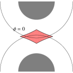
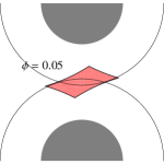
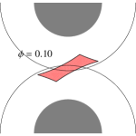
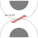
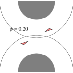
Figure 5: Possible positions of the center of mass $(x,y)$ for different values of $\phi$, see equation (11), at a binary collision event. Here $\rho=13/25l$ and $\rho_{\mathrm{m}}=13/50l$.

As seen from figure 5, the area is connected for $-\phi_{\mathrm{T}}\leq\phi\leq\phi_{\mathrm{T}}$, where $\phi_{\mathrm{T}}$ is the angle $\phi$ at which opposite arcs intersect,

$$\phi_{\mathrm{T}}=\arcsin\frac{\rho_{\mathrm{m}}^{2}-\rho_{\mathrm{c}}^{2}}{l\rho_{\mathrm{m}}}.$$ (14)

Beyond that value, the area splits into two triangular areas. These areas shrink to zero at the angle $\phi$ given by

$$\phi_{\mathrm{M}}=\arccos\frac{\rho_{\mathrm{m}}\rho_{\mathrm{c}}+l/2\sqrt{\rho^{2}-\rho_{\mathrm{m}}^{2}}}{\rho^{2}}.$$ (15)

Let $-\phi_{\mathrm{M}}\leq\phi\leq\phi_{\mathrm{M}}$. We denote by $x_{1}<x_{2}<x_{3}<x_{4}$ the four corners of the rectangular domain,

$$\begin{array}[]{lcl}x_{1}&=&-x_{4}=-2(\rho_{\mathrm{m}}\cos\phi-\rho_{\mathrm{c}}),\\ x_{2}&=&-x_{3}=-2\sqrt{\rho^{2}-\rho_{\mathrm{m}}^{2}}\sin\phi.\end{array}$$ (16)

For $\phi\geq\phi_{\mathrm{T}}$, the points at which the opposite arcs intersect are given by

$$x_{i}=\pm(l-2\rho_{\mathrm{m}}\sin\phi)\left[\frac{-l^{2}+4l\rho_{\mathrm{m}}\sin\phi+4(\rho^{2}-\rho_{\mathrm{m}}^{2})}{l^{2}-4l\rho_{\mathrm{m}}\sin\phi+4\rho_{\mathrm{m}}^{2}}\right]^{1/2}.$$ (17)

Combining equations (13)-(17) together, we can make use of the symmetry $\phi\to-\phi$ and write the integral to be computed as

$$\alpha(\rho,\rho_{\mathrm{m}})\equiv\int\/\mathrm{d}\/\phi\/\mathrm{d}\/\bi{R}=2\left[\int_{0}^{\phi_{\mathrm{M}}}A_{1}(\phi)\/\mathrm{d}\/\phi+\int_{\phi_{\mathrm{T}}}^{\phi_{\mathrm{M}}}A_{2}(\phi)\/\mathrm{d}\/\phi\right],$$ (18)

where

$$A_{1}(\phi)=\int_{x_{1}}^{x_{3}}y_{+1,-1}(x)\/\mathrm{d}\/x+\int_{x_{3}}^{x_{4}}y_{-1,-1}(x)\/\mathrm{d}\/x-\int_{x_{1}}^{x_{2}}y_{+1,+1}(x)\/\mathrm{d}\/x-\int_{x_{2}}^{x_{4}}y_{-1,+1}(x)\/\mathrm{d}\/x,$$ (19)

which is the area bounded by the four arcs $y_{\sigma,\tau}$, and

$$A_{2}(\phi)=\int_{-x_{i}}^{x_{i}}[y_{-1,+1}(x)-y_{+1,-1}(x)]\/\mathrm{d}\/x,$$ (20)

is the area of the overlapping opposite arcs $y_{-1,+1}$ and $y_{+1,-1}$, which occurs when $\phi_{\mathrm{T}}\leq\phi\leq\phi_{\mathrm{M}}$ [it gives a negative contribution to $A_{1}(\phi)$].

The computation of these expressions is easily performed numerically, and the result shown in figure 6.

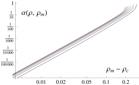
Figure 6: Area of binary collisions $\alpha(\rho,\rho_{\mathrm{m}})$ versus $\rho_{\mathrm{m}}-\rho_{\mathrm{c}}$ for seven values of $\rho$ ranging from $9/25$ to $42/100$ ($l=1/\sqrt{2}$).

Near the critical geometry, we expand the quantity (18) in powers of the difference $\rho_{\mathrm{m}}-\rho_{\mathrm{c}}$,

$$\alpha(\rho,\rho_{\mathrm{m}}\big{)}=\sum_{n=1}^{\infty}c_{n}(\rho_{\mathrm{m}}-\rho_{\mathrm{c}})^{n}.$$ (21)

The first two coefficients vanish, so that the leading term corresponds to $n=3$. The first few coefficients are derived in B and given by :

$$\eqalign{c_{1}=c_{2}=0,\\ c_{3}=\frac{128\rho_{\mathrm{c}}}{3l^{2}},\\ c_{4}=\frac{256\rho_{\mathrm{c}}^{2}}{3l^{4}},\\ c_{5}=\frac{16}{l^{2}}\left(\frac{1}{3\rho_{\mathrm{c}}}+\frac{8\rho_{\mathrm{c}}}{5l^{2}}+\frac{16\rho_{\mathrm{c}}^{3}}{l^{4}}+\frac{16\rho^{4}}{5l^{4}\rho_{\mathrm{c}}}\right).}$$ (22)

We further note that the computation of the two-cell 4-volume, $|\mathcal{L}_{\rho,\rho_{\mathrm{m}}}(2)|$, which, as noticed above, is approximated by the square of the single cell area $|\mathcal{B}_{\rho}|^{2}$, can be improved using equation (21). Indeed it is easily seen that $\/\mathrm{d}\/|\mathcal{L}_{\rho,\rho_{\mathrm{m}}}(2)|/\/\mathrm{d}\/\rho_{\mathrm{m}}=-2\alpha(\rho,\rho_{\mathrm{m}})$, which implies

$$|\mathcal{L}_{\rho,\rho_{\mathrm{m}}}(2)|=|\mathcal{B}_{\rho}|^{2}-2\sum_{n=4}^{\infty}\frac{c_{n-1}}{n}(\rho_{\mathrm{m}}-\rho_{\mathrm{c}})^{n}.$$ (23)

It is immediate to check that corrections $|\mathcal{L}_{\rho,\rho_{\mathrm{m}}}(2)|-|\mathcal{B}_{\rho}|^{2}=\mathcal{O}(\rho_{\mathrm{m}}-\rho_{\mathrm{c}})^{4}$.

3.3 Binary collision frequency

Having computed the transition rates of the master equation with respect to the billiard geometry, we now turn to the computation of observables. The first quantity of interest, which can be readily computed from equation (10), is the binary collision frequency $\nu_{\mathrm{b}}$. This is an equilibrium quantity which, in the (global) microcanonical ensemble with energy $E=\epsilon_{1}+\dots+\epsilon_{N}$, involves the two-particle energy distribution,

$$P^{(\mathrm{eq})}_{2}(\epsilon_{a},\epsilon_{b})=\frac{(N-1)(N-2)}{E^{2}}\left(1-\frac{\epsilon_{a}+\epsilon_{b}}{E}\right)^{N-3},$$ (24)

and can be written as

$$\nu_{\mathrm{b}}=\int\/\mathrm{d}\/\epsilon_{a}\,\/\mathrm{d}\/\epsilon_{b}\,\/\mathrm{d}\/\eta\,W(\epsilon_{a},\epsilon_{b}|\epsilon_{a}-\eta,\epsilon_{b}+\eta)P^{(\mathrm{eq})}_{2}(\epsilon_{a},\epsilon_{b}).$$ (25)

Taking the large $N$ limit and letting $E=Nk_{\mathrm{B}}T\equiv N/\beta$, we can write $P^{(\mathrm{eq})}_{2}(\epsilon_{a},\epsilon_{b})\simeq\beta^{2}\exp[-\beta(\epsilon_{a}+\epsilon_{b})][1+\mathcal{O}(N^{-1})]$. Substituting this expression into the above equation and inserting the expression of $W$ from equation (10), we obtain, after some calculations,

$$\nu_{\mathrm{b}}\simeq\sqrt{\frac{k_{\mathrm{B}}T}{\pi m}}\frac{2\rho_{\mathrm{m}}}{|\mathcal{B}_{\rho}|^{2}}\left(\int\/\mathrm{d}\/\phi\/\mathrm{d}\/\bi{R}\right)[1+\mathcal{O}(N^{-1})].$$ (26)

This expression involves the geometric factor (18) in the first bracket. The leading term in the second bracket is the canonical expression of the binary collision frequency. The second term is a positive finite $N$ correction, which is useful in that it shows that the binary collision frequency decreases to its asymptotic value as $N\to\infty$.

3.4 Rescaled master equation

The binary collision frequency (26) defines a natural dimensionless time scale for the stochastic process described by the master equation (9) with transition rates (10). The master equation can thus be converted to dimensionless form by rescaling the energies by a reference thermal energy and time by the corresponding asymptotic ($N\to\infty$) value of the binary collision frequency (26).

Introducing the variables

$$e_{a} \equiv \frac{\epsilon_{a}}{k_{\mathrm{B}}T},$$ (27)

$$h \equiv \frac{\eta}{k_{\mathrm{B}}T},$$ (28)

$$\tau \equiv \nu_{\mathrm{b}}t,$$ (29)

equation (9) becomes

$$\partial_{\tau}p^{(\mathrm{leq})}_{N}(e_{1},\dots,e_{N},\tau)=\frac{1}{2}\sum_{a,b=1}^{N}\int\/\mathrm{d}\/h$$

$$\hbox to0.0pt{\hss${}\times{}$}\Big{[}w(e_{a}+h,e_{b}-h|e_{a},e_{b})\;p^{(\mathrm{leq})}_{N}(\dots,e_{a}+h,\dots,e_{b}-h,\dots,\tau)$$

$$-w(e_{a},e_{b}|e_{a}-h,e_{b}+h)\;p^{(\mathrm{leq})}_{N}(\dots,e_{a},\dots,e_{b},\dots,\tau)\Big{]},$$ (30)

with the transition rates

$$w(e_{a},e_{b}|e_{a}-h,e_{b}+h) = \sqrt{\frac{2}{\pi^{3}}}\int_{x_{1\|}-x_{2\|}>0}\/\mathrm{d}\/x_{1\|}\,\/\mathrm{d}\/x_{1\bot}\,\/\mathrm{d}\/x_{2\|}\,\/\mathrm{d}\/x_{2\bot}\,(x_{1\|}-x_{2\|})$$

$$\qquad\times\delta(e_{a}-x_{1\|}^{2}-x_{1\bot}^{2})\,\delta(e_{b}-x_{2\|}^{2}-x_{2\bot}^{2})\,\delta(h-x_{1\|}^{2}+x_{2\|}^{2})$$

This master equation shows that all the properties of heat conduction are rescaled by the binary collision frequency and temperature in its limit of validity where the collision frequency vanishes. In particular, this shows that the coefficient of heat conduction is proportional to the binary collision frequency in this limit, as explained in the next subsection.

3.5 Thermal conductivity

Starting from the master equation (9), we derive an equation for the evolution of the kinetic energy of each moving particle, $\langle\epsilon_{a}\rangle\equiv k_{\mathrm{B}}T_{a}$, which defines the local temperature, where $\langle.\rangle$ denotes an average with respect to the energy distributions. By the structure of equation (9), such an equation can be expressed in terms of the transfer of energy due to the binary collisions between neighbouring cells. The time evolution of the average local kinetic energy is given by

$$\partial_{t}\langle\epsilon_{a}\rangle=-\sum_{b}\langle J_{a,b}(\epsilon_{a},\epsilon_{b})\rangle,$$ (32)

with the energy flux defined as

$$\eqalign{J_{a,b}(\epsilon_{a},\epsilon_{b})\equiv\int\/\mathrm{d}\/\eta\,\eta\,W(\epsilon_{a},\epsilon_{b}|\epsilon_{a}-\eta,\epsilon_{b}+\eta),\\ \phantom{J_{a,b}(\epsilon_{a},\epsilon_{b})}=-\int\/\mathrm{d}\/\eta\,\eta\,W(\epsilon_{a}+\eta,\epsilon_{b}-\eta|\epsilon_{a},\epsilon_{b}).}$$ (33)

This expresses the local conservation of energy.

Over long time scales, the probability distribution becomes controlled by this local conservation of energy, the slowest variables being the local kinetic energies $\langle\epsilon_{a}\rangle$ or, equivalently, the local temperatures $T_{a}$ as defined above. This holds even though statistical correlations develop between the local energies in the probability distributions. These statistical correlations are well known for transport processes ruled by master equations such as Eq. (9) [19, 23] and are observed in the present system as well.

To be specific, we consider a one-dimensional chain, extending along the $x$-axis, formed with a succession of pairs of rhombic billiard cells arranged in quincunx, similarly to the middle panel of figure 4, except the vertical height is here only one unit of length. The unit of horizontal and vertical lengths is thus $l\sqrt{2}$ and there are two cells per each unit of length. Similar results hold for different choices of geometry modulo straightforward adaptations.

We imagine that the system is in a non-equilibrium state, with a small temperature difference $\delta T$ about an average temperature $T$ between neighbouring cells, and consider the average heat transfered from cell $a$ at inverse temperature $\beta_{a}=\beta+\delta\beta/2$ to cell $b$ at inverse temperature $\beta_{b}=\beta-\delta\beta/2$, $\delta\beta=-\delta T/(k_{\mathrm{B}}T^{2})$, both cells being assumed to be in thermal equilibrium at their respective temperatures. The statistical correlations we observe in the present system are of the order of $\delta\beta^{2}$, as it is the case in other systems [19]. In the non-equilibrium state, these statistical correlations are controlled in the long-time limit by the local temperatures. Since the process is here ruled by a Markovian master equation in the limit of small binary collision frequency, we get the equation of heat for the temperature

$$\partial_{t}T(x,t)=\partial_{x}[\kappa\partial_{x}T(x,t)],$$ (34)

where the local temperature is here written as $T(x,t)=\langle\epsilon_{ij}\rangle/k_{\mathrm{B}}$, $x=\sqrt{2}l(i+j/2)$, $i=1,\dots,N/2$, $j=0,1$ [see equation (1)].

According to the rescaling property of the master equation discussed in section 3.4, the heat conductivity is proportional to the binary collision frequency  :

$$\frac{\kappa}{l^{2}}=A\,\nu_{\mathrm{b}},$$ (35)

with a dimensionless constant $A$.

An analytical estimation can be obtained by transforming the master equation into a hierarchy of equations for all the moments of the probability distribution: $\langle\epsilon_{a}\rangle$, $\langle\epsilon_{a}\epsilon_{b}\rangle$, $\langle\epsilon_{a}\epsilon_{b}\epsilon_{c}\rangle$,… The evolution equations of these moments are coupled.

Truncating the hierarchy at the equations for the averages $\langle\epsilon_{a}\rangle$, we get the approximate heat conductivity :

$$\frac{\kappa}{l^{2}} \simeq\frac{\beta^{4}}{2}\int\/\mathrm{d}\/\epsilon_{a}\/\mathrm{d}\/\epsilon_{b}\/\mathrm{d}\/\eta\ \eta(\epsilon_{b}-\epsilon_{a})W(\epsilon_{a},\epsilon_{b}|\epsilon_{a}-\eta,\epsilon_{b}+\eta)\exp[-\beta(\epsilon_{a}+\epsilon_{b})],$$ (36)

$$=\sqrt{\frac{k_{\mathrm{B}}T}{\pi m}}\frac{2\rho_{\mathrm{m}}}{|\mathcal{B}_{\rho}|^{2}}\left(\int\/\mathrm{d}\/\phi\/\mathrm{d}\/\bi{R}\right).$$

So that $A=1$ in this approximation. The same result holds if we include the equations for the moments $\langle\epsilon_{a}\epsilon_{b}\rangle$ with $|a-b|\leq 1$.

Though the approximate result (36) above does not rule out possible corrections to $A=1$, we argue that $A=1$ is an exact property of the master equation (9) in the infinite system limit. This claim is borne out by extensive studies of the stochastic process described by equation (9) that will be reported in a separate publication [24]. The focus is here on the billiard systems whose conductivity may however bear corrections to this identity, due we believe to lack of sufficient separation of time scales between wall and binary collision events. In the following, the results of numerical computations are presented which support these claims.

4 Numerical results

The above formulae for the binary collision frequency, equation (26), and the thermal conductivity, equation (36), together with the expressions of the geometric factors, equations (22) and (23), provide a detailed picture of the mechanism which governs the transport of heat in our model. Numerical computations of these quantities further add to this picture and provide strong evidence of the validity of our theoretical approach.

4.1 Binary and wall collision frequencies

For the sake of computing the binary collision frequency, we simulate the quasi-one dimensional channel of $N$ cells with rhombic shapes and apply periodic boundary conditions at the horizontal ends of the channel. Thus each cell has two neighbouring cells, left and right, and interactions between any two neighbouring cells can occur through both top and bottom corners .

In figure 7, we compare the computations of $\nu_{\mathrm{b}}$ to $\nu_{\mathrm{w}}$ for a system of $N=10$ cells at unit temperature. The parameters are taken to be $\rho=9/25$ and $\rho_{\mathrm{m}}=3/25,\dots,17/50$ by steps of $1/50$. Both collision frequencies are computed in the units of the microcanonical average velocity, $\overline{v}_{\mathrm{N}}\equiv 2^{N}\sqrt{N/2}(N-1)!/(2N-1)!!$, which, as $N\to\infty$, converges to the canonical average velocity $\overline{v}_{\infty}=\sqrt{\pi/2}$. The wall collision frequency is compared to the collision frequency of the isolated cells $\nu_{\mathrm{c}}$, itself measured in the units of the single particle velocity. As expected, $\nu_{\mathrm{b}}/\nu_{\mathrm{w}}\ll 1$ and $\nu_{\mathrm{w}}\simeq\nu_{\mathrm{c}}$ for $\rho_{\mathrm{m}}\gtrsim\rho_{\mathrm{c}}$. The crossover $\nu_{\mathrm{b}}\simeq\nu_{\mathrm{w}}$ occurs at $\rho_{\mathrm{m}}\simeq 11/50$ for this value of $\rho$.

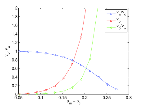
Figure 7: Wall and binary collision frequencies $\nu_{\mathrm{w}}$ and $\nu_{\mathrm{b}}$ versus $\rho_{\mathrm{m}}-\rho_{\mathrm{c}}$ in a one-dimensional channel of $N=10$ rhombic cells with $\rho=9/25$ and lattice spacing $l=1/\sqrt{2}$.

4.2 Thermal conductivity

4.2.1 Heat flux.

The thermal conductivity can be obtained by computing the heat flux in a nonequilibrium stationary state. Such stationary states occur when the two ends of the channel are put in contact with heat baths at separate temperatures, say $T_{-}$ and $T_{+}$, $T_{-}<T_{+}$.

Let a system of $N$ cells be in contact with two thermostated cells at respective temperatures $T_{\pm}$, and let these cell indices be $n=\pm(N+1)/2$ (we take $N$ odd for the sake of definiteness). Provided the difference between the bath temperatures is small, $T_{+}-T_{-}\ll(T_{+}+T_{-})/2$, a linear gradient of temperature establishes through the system, with local temperatures

$$T_{n}=\frac{1}{2}(T_{+}+T_{-})+\frac{n}{N+1}(T_{+}-T_{-}).$$ (37)

Under these conditions, the nonequilibrium stationary state is expected to be locally well approximated by a canonical equilibrium at temperature $T_{n}$.

This can be checked numerically. In fact the local thermal equilibrium is verified (by comparing the moments of $\epsilon_{n}$ to their Gaussian expectation values) under the weaker property of small local temperature gradients, i. e. $(T_{+}-T_{-})/N\ll(T_{+}+T_{-})/2$, for which the temperature profile is generally not linear since the thermal conductivity depends on the temperature. Indeed, since $\kappa\propto T^{1/2}$, we expect in that case, according to Fourier’s law, the profile

$$T_{n}=\left[\frac{1}{2}(T_{-}^{3/2}+T_{+}^{3/2})+\frac{n}{N+1}(T_{+}^{3/2}-T_{-}^{3/2})\right]^{2/3}.$$ (38)

The thermal conductivity can therefore be computed from the heat exchanges of the chain in contact with the two cells at the ends of the chain, respectively thermalized at temperatures $T\pm\delta T/2$, $\delta T\ll T$. The thermalization of the end cells is achieved by randomizing the velocities of the two particles at every collision they make with their cells walls, according to the usual thermalization procedure of particles colliding with thermalized walls [28].

First, we consider a chain containing a single cell in order to test the validity of the master equation. In this case, the procedure amounts to simulating a single particle confined to its cell and performing random collisions with stochastic particles which penetrate the cell corners according to the statistics of binary collisions. For a chain with a single cell, the heat conductance is given by Eq. (36) with $A=1$, as there are no correlations with the stochastic particles.

Figure 8 shows the results of the computations of the heat conductance with this method and provides a comparison with the binary collision frequency $\nu_{\mathrm{b}}$ on the one hand (left panel), as well as with the results of our kinetic theory predictions on the other hand (right panel).

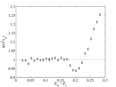
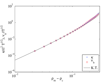
Figure 8: Reduced thermal conductance $\kappa$, computed from the heat exchange in a chain with a single particle with thermalized neighbours, and binary collision frequency $\nu_{\mathrm{b}}$, as functions of $\rho_{\mathrm{m}}-\rho_{\mathrm{c}}$. (Left) ratio between $\kappa$ and $\nu_{\mathrm{b}}$; (Right) comparison with the results of section 3. The only relevant parameter is $\rho=9/25$. For each value of $\rho_{\mathrm{m}}$, several temperature differences $\delta T$ were taken, all giving consistent values of $\kappa$. The solid line shows the result of kinetic theory (K.T.).

The agreement between the data and equations (26), (36), (35) and the computation of the integrals (18)-(20), especially as $\rho_{\mathrm{m}}\to\rho_{\mathrm{c}}$, demonstrates the validity of the stochastic description of the billiard system, equation (9).

Next, we increase the size of the chain in order to reach the thermal conductivity in the limit of an arbitrarily large chain. The results are that statistical correlations appear between the kinetic energies along the chain. As we show below, their influence on the computed value of the conductivity diminishes as $\rho_{\mathrm{m}}\to\rho_{\mathrm{c}}$.

Fix $T_{-}=0.5$ and $T_{+}=1.5$ to be the baths temperatures, and let the size of the system increase from $N=1$ to $N=20$ as $\rho_{\mathrm{m}}$ is progressively decreased from $\rho_{\mathrm{m}}=11/50$ to $\rho_{\mathrm{m}}=13/100$, with fixed $\rho=9/25$. As one can see from figure 8, this range of values of $\rho_{\mathrm{m}}$ crosses over from a regime where the separation of time scales is not effective to one where it appears to be and where the stochastic model should therefore be a reasonable approximation to the process of energy transport in the billiard.

For all values of $\rho_{\mathrm{m}}$, we measured the temperature profile and heat fluxes throughout the system and inferred the value of the reduced thermal conductivity by linearly extrapolating the ratios between the average heat flux and local temperature gradient divided by the square root of the local temperature as functions of $1/N$ to the vertical axis intercept, corresponding to $N=\infty$. Given the parameter values, every realisation was carried out over a time corresponding to 1,000 interactions between the system and baths and repeated over $10^{4}$ realisations. For $N$ up to 20, this time provided satisfying stationary statistics, with temperature profiles verifying equation (38) and statistically constant heat fluxes.

The results of the linear regression used to compute the value of $\kappa/\nu_{\mathrm{b}}$ for selective values of $\rho_{\mathrm{m}}$ are shown in figures 9 and 10.

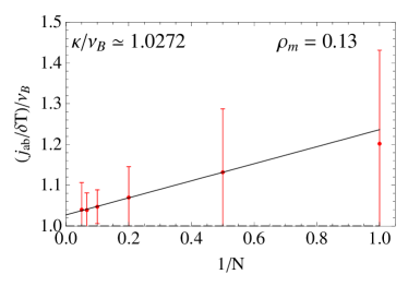
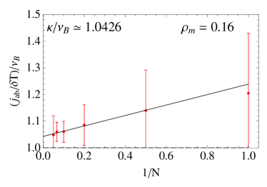
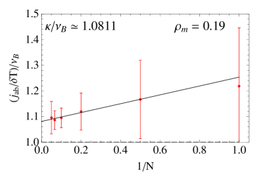
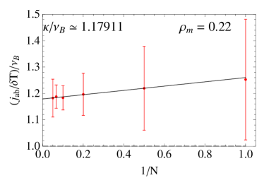
Figure 9: Ratio between thermal conductivity and binary collision frequency, $\kappa/\nu_{\mathrm{b}}$, extrapolated from the computation of the average ratio between heat current and local temperature gradients, divided by the local binary collision frequency, $1/n\sum_{i}[J_{i,i+1}/(T_{i+1}-T_{i})]/\nu_{\mathrm{b}}(i)$. The system sizes are $N=1,2,5,10,15,20$. The four pannels correspond to different values of $\rho_{\mathrm{m}}=13/100,4/25,19/100,11/50$, with $\rho=9/25$ and thus $\rho_{\mathrm{c}}\simeq 0.068$. The red dots are the data points with corresponding error bars and the black solid line shows the result of a linear regression performed with data associated to systems of lengths $N\geq 2$.

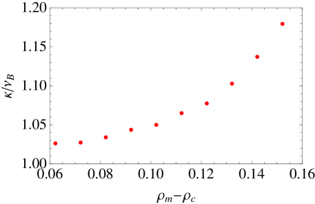
Figure 10: Ratio between thermal conductivity and binary collision frequency, $\kappa/\nu_{\mathrm{b}}$, computated as in figure 9, here collected for a larger set of values of $\rho_{\mathrm{m}}$. The horizontal axis shows the difference $\rho_{\mathrm{m}}-\rho_{\mathrm{c}}$. The error bars are of the same order as those in figure 8, with deviations from unity of the data points of the same order as those in the latter figure.

Our results thus make it plausible that the ratio between the thermal conductivity and binary collision frequency approaches unity as the parameter $\rho_{\mathrm{m}}$ decreases towards the critical value $\rho_{\mathrm{c}}$. As will be show in a separate publication [24], this is indeed a property of the stochastic model described by equation (9) and has been verified numerically by direct simulation of the master equation within an accuracy of 4 digits. As of the billiard system, it is unfortunately difficult to improve the results beyond those presented here as the CPU times necessary to either increase $N$ or decrease $\rho_{\mathrm{m}}$ quickly become prohibitive. Nevertheless, the data displayed in figures 9 and 10 offer convincing evidence that the thermal conductivity is well approximated by the binary collision frequency so long as the separation of time scales between wall and binary collision events is effective.

4.2.2 Helfand moment.

The computation of the thermal conductivity can also be performed in the global equilibrium microcanonical ensemble using the method of Helfand moments [25, 26, 27].

The Helfand moment has expression $H(t)=\sum_{a}x_{a}(t)\epsilon_{a}(t)$, where $x_{a}(t)$ denotes the horizontal position of particle $a$ at time $t$ and $\epsilon_{a}(t)=|\bi{v}_{a}(t)|^{2}/2$ its kinetic energy (the masses are taken to be unity). The computation of the time evolution of this quantity proceeds by discrete steps, integrating the Helfand moment from one collision event to the next, whether between a particle and the walls of its cell, or between two particles. Let $\{\tau_{n}\}_{n\in\mathbb{Z}}$ denote the times at successive collision events. In the absence of binary collisions, the energies are locally conserved and the Helfand moment changes according to $H(\tau_{n})=H(\tau_{n-1})+\sum_{a}[x_{a}(\tau_{n})-x_{a}(\tau_{n-1})]\epsilon_{a}(\tau_{n-1})$. If, on the other hand, a binary collision occurs between particles $k$ and $l$, the Helfand moment changes by an additional term $[x_{k}(\tau_{n})-x_{l}(\tau_{n})][\epsilon_{k}(\tau_{n}+0)-\epsilon_{k}(\tau_{n}-0)]$. Computing the time average of the squared Helfand moment, we obtain an expression of the thermal conductivity according to

$$\kappa=\lim_{L\to\infty}\frac{1}{L(k_{\mathrm{B}}T)^{2}}\lim_{n\to\infty}\frac{1}{2\tau_{n}}\Big{\langle}[H(\tau_{n})-H(\tau_{0})]^{2}\Big{\rangle}$$ (39)

where $L=N/2$ is the horizontal length of the system.

Figure 11 shows the results of a computation of the thermal conductivity through equation (39) for different system sizes. Though the actual values of $\kappa$ vary wildly with $N$, it is clear that a finite asymptotic value is reached for $N\simeq 10^{2}$. In this case, the constant of proportionality in equation (35) takes the value $A=0.98\pm 0.08$, close to 1. Similar results were obtained for other parameter values, and other cell geometries as well.

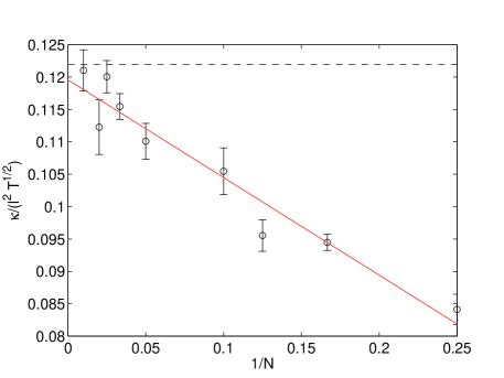
Figure 11: Reduced thermal conductivity, computed from the mean squared Helfand moment, versus $1/N$. The parameters are $\rho=9/25$, $\rho_{\mathrm{m}}=9/50$. The system sizes vary from $N=4$ to $N=100$. The dashed line shows the binary collision frequency, $\nu_{\mathrm{b}}\simeq 0.1225$. The solid line shows a linear fit of the data, with $y$-intercept $0.12\pm 0.01$, in agreement with the prediction (35).

5 Lyapunov spectrum

A key aspect of our model, which justifies the assumption of local equilibrium, is that it is strongly chaotic. This property can be illustrated through the computation of the Lyapunov spectrum and Kolmogorov-Sinai entropy in equilibrium conditions.

As mentioned earlier, in the absence of interaction between the cells, $\rho_{\mathrm{m}}<\rho_{\mathrm{c}}$, The Lyapunov spectrum of a system of $N$ cells has $N$ positive and $N$ negative Lyapunov exponents, which, if divided by the average speed of the particle to which they are attached, are all equal in absolute value. This reference value we denote by $\lambda_{+}$. The $2N$ remaining Lyapunov exponents vanish.

As we increase $\rho_{\mathrm{m}}$ and let the particles interact, we expect that, in the regime $0<\rho_{\mathrm{m}}-\rho_{\mathrm{c}}\ll 1$, where binary collision events are rare, the Lyapunov exponents will essentially be determined by $\lambda_{+}$ multiplied by a factor which is specified by the particle velocities. The exchange of velocities thus produces an ordering of the exponents which can be computed as shown below. We note that the other half of the spectrum, which remains zero in this approximation, will only pick up positive values as a result of the interactions.

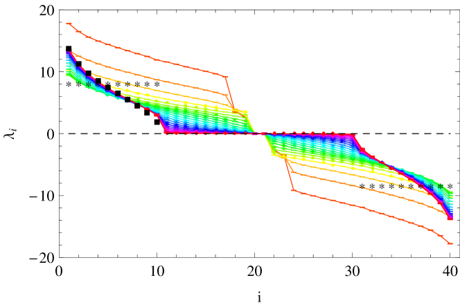
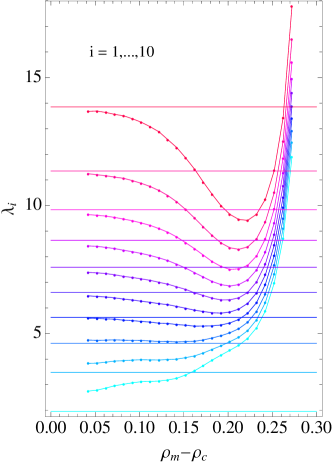
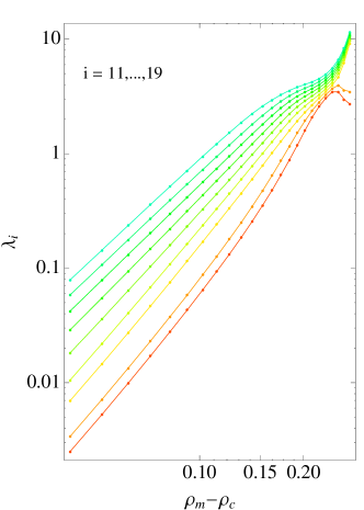
Figure 12: (Top) Lyapunov exponents $\lambda_{i}$ versus $i$ computed with a rhombic channel of size $N=10$ cells and parameter $\rho=9/25$. The different curves correspond to different values of $\rho_{\mathrm{m}}=0.11$ (bottom curve) to $0.34$ (top curve) by steps of $0.01$. The lines of stars are obtained for $\rho_{\mathrm{m}}=0.04<\rho_{\mathrm{c}}$, yielding the exponents $\lambda_{+}$ and $\lambda_{-}$ associated to isolated cells, with all the particles at the same speed. The squares correspond to the first half of the spectrum as predicted by equation (42). (Bottom) $\lambda_{i}$ versus $\rho_{\mathrm{m}}-\rho_{\mathrm{c}}$. The first of the two figures displays the first half of the positive part of the spectrum of exponents, $\lambda_{1},\dots,\lambda_{N}$ and compares them to the asymptotic estimate equation (42) (straight lines). The second plot shows the second half of the positive part of the spectrum, $\lambda_{N+1},\dots,\lambda_{2N-1}$, displaying their power-law scaling to zero as $\rho_{\mathrm{m}}\to\rho_{\mathrm{c}}$.

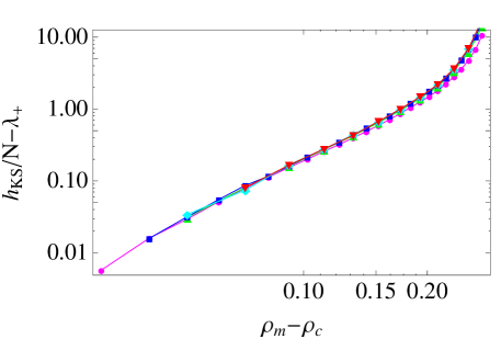
Figure 13: Extensivity of the Kolmogorov-Sinai entropy. The vertical axis shows the difference between the Kolmogorov Sinai entropy, here computed from the sum of the positive Lyapunov exponents for system sizes $N=3$ (magenta circles), $5$ (blue up triangles), $10$ (green squares), $15$ (cyan diamonds), $20$ (red down triangles), divided by the corresponding microcanonical average velocity, and the Lyapunov exponent of the isolated billiard cell at unit velocity. The curves fall nicely upon each other and converge to zero as $\rho_{\mathrm{m}}\to\rho_{\mathrm{c}}$.

Assume for the sake of the argument that $N$ is large. The probability that a given particle with velocity $v$ has exponent $\lambda=v\lambda_{+}$ less than a value $\lambda_{i}=v_{i}\lambda_{+}$ can be approximated by the probability that the particle velocity be less than $v_{i}$, which, if we assume a canonical form of the equilibrium distribution, is

$$\mathrm{Prob}(\lambda<\lambda_{i}) =\mathrm{Prob}(v<v_{i}),$$ (40)

$$=\beta\int_{0}^{mv_{i}^{2}/2}\/\mathrm{d}\/\epsilon\exp(-\beta\epsilon),$$

$$=1-\exp(-\beta mv_{i}^{2}/2).$$

But this probability is simply $(N-i+1/2)/N$. Therefore the half of the positive Lyapunov exponent spectrum, which is associated to the isolated motion of particles within their cells, becomes, in the presence of rare collision events,

$$\lambda_{i}=\lambda_{+}\sqrt{\frac{2}{m\beta}}\left[\ln\frac{N}{i-1/2}\right]^{1/2},\quad i=1,\dots,N,$$ (41)

with ordering $\lambda_{1}>\lambda_{2}>\dots>\lambda_{N}$. In particular, the largest exponent $\lambda_{1}$ grows like $\sqrt{\ln N}$. The Kolmogorov-Sinai entropy on the other hand is extensive : $h_{\mathrm{KS}}=N\lambda_{+}\sqrt{\pi/(2m\beta)}$.

Refined expressions can be computed by taking the microcanonical distribution associated to a finite $N$. In particular, the expressions of the Lyapunov exponents become

$$\lambda_{i}=\lambda_{+}\sqrt{\frac{2N}{m\beta}}\left[1-\left(\frac{i-1/2}{N}\right)^{1/(N-1)}\right]^{1/2}.$$ (42)

We mention in passing that similar arguments are relevant and can be used to approximate the Lyapunov spectrum (actually half of it) of other models, such as a mixture of light and heavy particles [30].

Let us again insist that equations (41) and (42) account for only $N$ of the $2N-1$ positive Lyapunov exponents. $N-1$ are vanishing within this approximation. For all these Lyapunov exponents, we expect the corrections to vanish with the binary collision frequency as we go to the critical geometry.

Figures 12 and 13 show the results of a numerical computation of the whole spectrum of Lyapunov exponents and corresponding Kolmogorov-Sinai entropy for the one-dimensional channel of rhombic cells. The agreement with equation (42) as $\rho_{\mathrm{m}}\to\rho_{\mathrm{c}}$ is very good, at the exception perhaps of the last few among the first $N$ exponents, whose convergence to the asymptotic value (42) appears to be slower. Interestingly, the largest exponents have a minimum which occurs at about the value of $\rho_{\mathrm{m}}$ for which the binary and wall collision frequencies have ratio unity, see figure 7. Indeed, for larger radii $\rho_{\mathrm{m}}$, the spectrum is similar to that of a channel of hard discs (without obstacles) [29]. Note that the same holds for the ratio between the thermal conductivity and binary collision frequency, as seen from figure 8. Thus one can interpret the occurrence of a minimum of the largest exponent as evidence of a crossover from a near close-packing solid-like phase ($\rho_{\mathrm{m}}\lesssim\rho$) to a gaseous-like phase trapped in a rigid structure ($\rho_{\mathrm{m}}\gtrsim\rho_{\mathrm{c}}$).

6 Conclusions

To summarize, lattice billiards form the simplest class of Hamiltonian models for which one can observe normal transport of energy, consistent with Fourier’s law. Geometric confinement restricts the transport properties of this system to heat conductivity alone, thereby avoiding the complications of coupling mass and heat transports, which are common to other many particle billiards.

The strong chaotic properties of the isolated billiard cells warrant, in a parametric regime where interactions among moving particles are seldom, the property of local equilibrium. This is to say, assuming that wall collision frequencies are order-of-magnitude larger than binary collision frequencies, that one is entitled to making a Markovian approximation according to which phase-space distributions are spread over individual cells. We are thus allowed to ignore the details of the distribution at the level of individual cells and coarse-grain the phase-space distributions to a many-particle energy distribution function, thereby going from the pseudo-Liouville equation, governing the microscopic statistical evolution, to the master equation, which accounts for the energy exchanges at a mesoscopic cell-size scale and local thermalization. The energy exchange process further drives the relaxation of the whole system to global equilibrium.

This separation of scales, from the cell scale dynamics, corresponding to the microscopic level, to the energy exchange among neighbouring cells at the mesoscopic level, and to the relaxation of the system to thermal equilibrium at the macroscopic level, is characterized by three different rates. The process of relaxation to local equilibrium has a rate given by the wall collision frequency, much larger than the rate of binary collisions, which characterizes the rate of energy exchanges which accompany the relaxation to local thermal equilibrium, itself much larger than the hydrodynamic relaxation rate, given by the binary collision rate divided by the square of the macroscopic length of the system.

On this basis, having reduced the deterministic dynamics of the many particles motions to a stochastic process of energy exchanges between neighboring cells, we are able to derive Fourier’s law and the macroscopic heat equation.

The energy transport master equation can be solved with the result, to be presented elsewhere [24], that the binary collision frequency and heat conductivity are equal. Under the assumption that the wall and binary collision time scales of the billiard are well separated, the transposition of this result to the billiard dynamics is that :

1. The heat conductivity of the mechanical model is proportional to the binary collision frequency, i. e. the rate of collisions among neighbouring particles,

   $$\frac{\kappa}{l^{2}\nu_{\mathrm{b}}}=A,\quad\nu_{\mathrm{b}}\ll\nu_{\mathrm{w}},$$

   with a constant $A$ that is exactly $1$ at the critical geometry, $\rho_{\mathrm{m}}\to\rho_{\mathrm{c}}$, where the evolution of probability densities is rigorously described by the master equation, and remains close to unity over a large range of parameter values for which we conclude the time scale separation is effective and the master equation therefore gives a good approximation to the energy transport process of the billiard ;

2. The heat conductivity and the binary collision frequency both vanish in the limit of insulating system, $\rho_{\mathrm{m}}\to\rho_{\mathrm{c}}$, with $(\rho_{\mathrm{m}}-\rho_{\mathrm{c}})^{3}$,

   $$\lim_{\rho_{\mathrm{m}}\to\rho_{\mathrm{c}}}\frac{\kappa}{l^{2}(\rho_{\mathrm{m}}-\rho_{\mathrm{c}})^{3}}=\lim_{\rho_{\mathrm{m}}\to\rho_{\mathrm{c}}}\frac{\nu_{\mathrm{b}}}{(\rho_{\mathrm{m}}-\rho_{\mathrm{c}})^{3}}=\frac{2\rho_{\mathrm{m}}}{|\mathcal{B}_{\rho}|^{2}}\sqrt{\frac{k_{\mathrm{B}}T}{\pi m}}c_{3},$$

   where the coefficient $c_{3}$ depends on the specific geometry of the binary collisions.

Though both results are exact strictly speaking only in the limit $\rho_{\mathrm{m}}\to\rho_{\mathrm{c}}$, the first one, according to our numerical computations, is robust and holds throughout the range of parameters for which the binary collision frequency is much less than the wall collision frequency, $\nu_{\mathrm{b}}\ll\nu_{\mathrm{w}}$. The deviations from $A=1$ which we observed at intermediary values of $\rho_{\mathrm{m}}$, where the separation of time scales is less effective, are interpreted as actual deviations of the energy transport process of the billiard from that described by the master equation, where correlations between the motions of neighboring particles must be accounted for.

Under the conditions of local equilibrium, the Lyapunov spectrum has a simple structure, half of it being determined according to random velocity distributions within the microcanonical ensemble, while the other half remains close to zero. The analytic expression of the Lyapunov spectrum that we obtained is thus exact at the critical geometry. The Kolmogorov-Sinai entropy is equal to the sum of the positive Lyapunov exponents and thus determined by half of them. It is extensive in the number of particles in the system, whereas the largest Lyapunov exponent grows like the square root of the logarithm of that number. As we mentioned earlier, we believe our method is relevant to the computation of the Lyapunov spectrum of other models of interacting particles [30]. The computation of the full spectrum, particularly regarding the effect of binary collisions on the exponents, remains an open problem.

Appendix A Computation of the Kernel

We provide in this appendix the explicit form of the transition rate $W$, given by equation (10).

We first substitute the two velocity integrals by two angle integrals, eliminating the two delta functions which involve only the local energies.

$$\int_{\hat{\bi{e}}_{ab}\cdot\bi{v}_{ab}>0}\hskip-9.95863pt\/\mathrm{d}\/\bi{v}_{a}\/\mathrm{d}\/\bi{v}_{b}\hat{\bi{e}}_{ab}\cdot\bi{v}_{ab}\ \delta\left(\epsilon_{a}-\frac{mv_{a}^{2}}{2}\right)\delta\left(\epsilon_{b}-\frac{mv_{b}^{2}}{2}\right)\delta\left(\eta-\frac{m}{2}[(\hat{\bi{e}}_{ab}\cdot\bi{v}_{a})^{2}-(\hat{\bi{e}}_{ab}\cdot\bi{v}_{b})^{2}]\right)$$

$$\hbox to0.0pt{\hss${}={}$}\frac{\sqrt{2}}{m^{5/2}}\int_{D_{+}}\/\mathrm{d}\/\theta_{a}\/\mathrm{d}\/\theta_{b}(\sqrt{\epsilon_{a}}\cos\theta_{a}-\sqrt{\epsilon_{b}}\cos\theta_{b})\delta(\eta-\epsilon_{a}\cos^{2}\theta_{a}+\epsilon_{b}\cos^{2}\theta_{b}),$$ (43)

where $\theta_{a/b}$ denote the angles of the velocity vectors $\bi{v}_{a/b}$ with respect to the direction $\phi$ of the relative position vector joining particles $a$ and $b$, $\hat{\bi{e}}_{ab}=(\cos\phi,\sin\phi)$, and the angle integration is performed over the domain $D_{+}$ such that $\sqrt{\epsilon_{a}}\cos\theta_{a}>\sqrt{\epsilon_{b}}\cos\theta_{b}$.

With the above expression (43), the explicit $\phi$ dependence has disappeared so that we have effectively decoupled the velocity integration from the integration over the direction of the relative position between the two colliding particles. We can further transform this expression in terms of Jacobian elliptic functions as follows.

Let $x_{i}=\cos\theta_{i}$, $i=a,b$, in equation (43), which becomes

$$\frac{4\sqrt{2}}{m^{5/2}}\int_{-1}^{1}\frac{\/\mathrm{d}\/x_{a}}{\sqrt{1-x_{a}^{2}}}\int_{-1}^{1}\frac{\/\mathrm{d}\/x_{b}}{\sqrt{1-x_{b}^{2}}}\theta(\sqrt{\epsilon_{a}}x_{a}-\sqrt{\epsilon_{b}}x_{b})(\sqrt{\epsilon_{a}}x_{a}-\sqrt{\epsilon_{b}}x_{b})\delta(\eta-\epsilon_{a}x_{a}^{2}+\epsilon_{b}x_{b}^{2}),$$ (44)

where $\theta(.)$ is the Heaviside step function. We thus have to perform the $x_{a}$ and $x_{b}$ integrations along the line defined by the argument of the delta function,

$$\eta=\epsilon_{a}x_{a}^{2}-\epsilon_{b}x_{b}^{2},$$ (45)

and that satisfies the condition

$$\sqrt{\epsilon_{a}}x_{a}>\sqrt{\epsilon_{b}}x_{b}.$$ (46)

To carry out this computation, we have to consider the following alternatives :

1. $\epsilon_{a}<\epsilon_{b}$, $0<\eta<\epsilon_{a}$
   The solution of equation (45) which is compatible with equation (46) is

   $$x_{a}=\left(\frac{\eta+\epsilon_{b}x_{b}^{2}}{\epsilon_{a}}\right)^{1/2}.$$ (47)

   Plugging this solution into equation (44) and setting the bounds of the $x_{b}$-integral to $\pm\sqrt{(\epsilon_{a}-\eta)/\epsilon_{b}}$, the expression (44) reduces to (omitting the prefactors)

   $$\int_{0}^{\sqrt{(\epsilon_{a}-\eta)/\epsilon_{b}}}\/\mathrm{d}\/x_{b}\frac{1}{\sqrt{\epsilon_{a}-\eta-\epsilon_{b}x_{b}^{2}}\sqrt{1-x_{b}^{2}}}=\frac{1}{\sqrt{\epsilon_{b}}}K\left(\frac{\epsilon_{a}-\eta}{\epsilon_{b}}\right),$$ (48)

   where $K$ denotes the Jabobian elliptic function of the first kind,

   $$K(m)=\int_{0}^{\pi/2}(1-m\sin^{2}\theta)^{-1/2}\/\mathrm{d}\/\theta\quad(m<1).$$ (49)

   Thus the kernel is, in this case,

   $$W(\epsilon_{a},\epsilon_{b}|\epsilon_{a}-\eta,\epsilon_{b}+\eta)=\frac{2\rho_{\mathrm{m}}}{\pi^{2}|\mathcal{L}_{\rho,\rho_{\mathrm{m}}}(2)|}\sqrt{\frac{2}{m\epsilon_{b}}}K\left(\frac{\epsilon_{a}-\eta}{\epsilon_{b}}\right)\int\/\mathrm{d}\/\phi\/\mathrm{d}\/\bi{R}.$$ (50)

2. $\epsilon_{a}<\epsilon_{b}$, $\epsilon_{a}-\epsilon_{b}<\eta<0$
   This case is similar to case (i), with equation (47) replaced by

   $$x_{b}=-\left(\frac{-\eta+\epsilon_{a}x_{a}^{2}}{\epsilon_{b}}\right)^{1/2}$$ (51)

   and $-1<x_{a}<+1$. The expression of the kernel corresponding to this case is therefore

   $$W(\epsilon_{a},\epsilon_{b}|\epsilon_{a}-\eta,\epsilon_{b}+\eta)=\frac{2\rho_{\mathrm{m}}}{\pi^{2}|\mathcal{L}_{\rho,\rho_{\mathrm{m}}}(2)|}\sqrt{\frac{2}{m(\epsilon_{b}+\eta)}}K\left(\frac{\epsilon_{a}}{\epsilon_{b}+\eta}\right)\int\/\mathrm{d}\/\phi\/\mathrm{d}\/\bi{R}.$$ (52)

3. $\epsilon_{a}<\epsilon_{b}$, $-\epsilon_{b}<\eta<\epsilon_{a}-\epsilon_{b}<0$
   This case is similar to case (ii), with $-\sqrt{(\epsilon_{b}+\eta)/\epsilon_{a}}<x_{a}<+\sqrt{(\epsilon_{b}+\eta)/\epsilon_{a}}$. In this case, the expression of the kernel is given by

   $$W(\epsilon_{a},\epsilon_{b}|\epsilon_{a}-\eta,\epsilon_{b}+\eta)=\frac{2\rho_{\mathrm{m}}}{\pi^{2}|\mathcal{L}_{\rho,\rho_{\mathrm{m}}}(2)|}\sqrt{\frac{2}{m\epsilon_{a}}}K\left(\frac{\epsilon_{b}+\eta}{\epsilon_{a}}\right)\int\/\mathrm{d}\/\phi\/\mathrm{d}\/\bi{R}.$$ (53)

The cases with $\epsilon_{a}>\epsilon_{b}$ are obtained from the cases above with the roles of $a$ and $b$ interchanged and $\eta\to-\eta$.

Appendix B Collision area near the critical geometry

The reason why $c_{1}$ and $c_{2}$ in equation (22) vanish is that the angle difference is $\mathcal{O}(\rho_{\mathrm{m}}-\rho_{\mathrm{c}})$ and the area $A_{1}(\phi)=\mathcal{O}[(\rho_{\mathrm{m}}-\rho_{\mathrm{c}})^{2}]$. These quantities are easily computed.

Let $\rho_{\mathrm{m}}=(1+\varepsilon)\rho_{\mathrm{c}}$, $\varepsilon\ll 1$. We have

$$\phi_{\mathrm{T}}=\frac{2\rho_{\mathrm{c}}}{l}\varepsilon-\frac{\rho_{\mathrm{c}}}{l}\varepsilon^{2}+\mathcal{O}(\varepsilon^{3}),$$ (54)

$$\phi_{\mathrm{M}}=\frac{2\rho_{\mathrm{c}}}{l}\varepsilon+\frac{4\rho_{\mathrm{c}}^{3}}{l^{3}}\varepsilon^{2}+\mathcal{O}(\varepsilon^{3}),$$ (55)

which indicates that the bounds of the angle integrals appearing in equation (18) are $\mathcal{O}(\varepsilon)$, with $\phi_{\mathrm{M}}$ and $\phi_{\mathrm{T}}$ differing only to $\mathcal{O}(\varepsilon^{2})$.

The leading contribution to the integral $\alpha(\rho,\rho_{\mathrm{m}})$ therefore stems only from the integration of $A_{1}(\phi)$, which we can compute explicitly by expanding $\rho_{\mathrm{m}}$ about $\rho_{\mathrm{c}}$ and taking into consideration that $\phi$ is $\mathcal{O}(\varepsilon)$. The result is

$$\int_{0}^{\phi_{\mathrm{M}}}A_{1}(\phi)\/\mathrm{d}\/\phi \simeq\int_{0}^{\phi_{\mathrm{T}}}A_{1}(\phi)\/\mathrm{d}\/\phi,$$ (56)

$$\simeq\int_{0}^{\phi_{\mathrm{T}}}\Big{(}\frac{16\rho_{\mathrm{c}}^{3}}{l}\varepsilon^{2}-4l\rho_{\mathrm{c}}\phi^{2}\Big{)}\/\mathrm{d}\/\phi,$$

$$=\frac{64\rho_{\mathrm{c}}^{4}}{3l^{2}}\varepsilon^{3},$$

which yields the leading coefficient $c_{3}$ in equation (22).

We can compute the coefficients of the next few powers in the expansion (21) in a similar fashion. First we notice that $A_{2}(\phi)$ is $\mathcal{O}(\varepsilon^{3})$ so that its integral between $\phi_{\mathrm{T}}$ and $\phi_{\mathrm{M}}$ is $\mathcal{O}(\varepsilon^{5})$. Therefore only the integral of $A_{1}(\phi)$ contributes to $c_{4}$ in equation (22).

The computation of the next terms in the expansion is more involved since it requires the integration of $A_{2}(\phi)$, whose expression is :

$$A_{2}(\phi)= 8\rho^{2}\arcsin\left[\frac{\rho_{\mathrm{m}}l\sin\phi-(\rho_{\mathrm{m}}^{2}-\rho_{\mathrm{c}}^{2})}{\rho^{2}}\right]^{1/2}$$

$$-4[\rho_{\mathrm{m}}l\sin\phi-(\rho_{\mathrm{m}}^{2}-\rho_{\mathrm{c}}^{2})]^{1/2}(4\rho_{\mathrm{m}}^{2}+l^{2}-4\rho_{\mathrm{m}}l\sin\phi)^{1/2}.$$

Expanding this expression for $\rho_{\mathrm{m}}$ $\varepsilon$-close to $\rho_{\mathrm{c}}$ and $\phi$ $\varepsilon^{2}$-close to $\phi_{\mathrm{T}}$, we get, to leading order,

$$\int_{\phi_{\mathrm{T}}}^{\phi_{\mathrm{M}}}A_{2}(\phi)\/\mathrm{d}\/\phi=\frac{1024\rho^{4}\rho_{\mathrm{c}}^{4}}{15l^{6}}\varepsilon^{5}.$$ (58)

Combining this expression with the 5$th$ order contribution to the integral of $A_{1}(\phi)$, we obtain $c_{5}$, equation (22). We point out that this coefficient is actually much larger than $c_{3}$ and $c_{4}$, a reason being that negative powers of $\rho_{\mathrm{c}}$ appear in its expression. The same holds of the next few coefficients.

References

- [1] Fourier J 1822 Théorie analytique de la chaleur (Didot, Paris); Reprinted 1988 (J Gabay, Paris); Facsimile available online at http://gallica.bnf.fr.
- [2] Bonetto F, Lebowitz J L, and Rey-Bellet L 2000 Fourier Law: A Challenge To Theorists in Fokas A, Grigoryan A, Kibble T, Zegarlinski B (Eds.) Mathematical Physics 2000 (Imperial College, London).
- [3] Bunimovich L A and Sinai Ya G 1980 Statistical properties of lorentz gas with periodic configuration of scatterers Commun. Math. Phys. 78 479.
- [4] Bunimovich L A and Spohn K 1996 Viscosity for a periodic two disk fluid: An existence proof Commun. Math. Phys. 176 661.
- [5] Machta J and Zwanzig R 1983 Diffusion in a Periodic Lorentz Gas Phys. Rev. Lett. 50 1959.
- [6] Gaspard P, Nicolis G, and Dorfman J R 2003 Diffusive Lorentz gases and multibaker maps are compatible with irreversible thermodynamics Physica A 323 294.
- [7] Mejía-Monasterio C, Larralde H, and Leyvraz F 2001 Coupled Normal Heat and Matter Transport in a Simple Model System Phys. Rev. Lett. 86 5417.
- [8] Eckmann J P and Young L S 2004 Temperature profiles in Hamiltonian heat conduction Europhys. Lett. 68 790.
- [9] Eckmann J P and Young L S 2006 Nonequilibrium energy profiles for a class of 1-D models Comm. Math. Phys. 262 237.
- [10] Eckmann J P, Mejía-Monasterio C, and Zabey E 2006 Memory Effects in Nonequilibrium Transport for Deterministic Hamiltonian Systems J. Stat. Phys. 123 1339.
- [11] Lin K K and Young L S 2007 Correlations in nonequilibrium steady states of random halves models J. Stat. Phys. 128 607.
- [12] Ravishankar K and Young L S 2007 Local thermodynamic equilibrium for some stochastic models of Hamiltonian origin J. Stat. Phys. 128 641.
- [13] Eckmann J P and Jacquet P 2007 Controllability for chains of dynamical scatterers Nonlinearity 20 1601.
- [14] Kupiainen A 2007 On Fourier s law in coupled lattice dynamics oral communication (Institut Henri Poincaré, Paris, France).
- [15] Bunimovich L, Liverani C, Pellegrinotti A, and Suhov Y 1992 Ergodic systems of balls in a billiard table Comm. Math. Phys. 146 357.
- [16] Dolgopyat D, Keller G, and Liverani C 2007 Random Walk in Markovian Environment, to appear in Annals of Probability; Dolgopyat D and Liverani C 2007 Random Walk in Deterministically Changing Environment preprint.
- [17] Bricmont J and Kupiainen A 2008 in preparation.
- [18] Gaspard P and Gilbert T 2008 Heat conduction and Fourier’s law by consecutive local mixing and thermalization Phys. Rev. Lett. 101 020601.
- [19] Nicolis G and Malek Mansour M 1984 Onset of spatial correlations in nonequilibrium systems: A master-equation description Phys. Rev. A 29 2845.
- [20] Chernov N and Markarian R 2006 Chaotic billiards Math. Surveys and Monographs 127 (AMS, Providence, RI).
- [21] Ernst M H, Dorfman J R, Hoegy W R, and Van Leeuwen J M J 1969 Hard-sphere dynamics and binary-collision operators Physica 45 127; Dorfman J R and Ernst M H 1989 Hard-sphere binary-collision operators J. Stat. Phys. 57 581.
- [22] Résibois P and De Leener M 1977 Classical kinetic theory of fluids (John Wiley & Sons, New York).
- [23] Spohn H 1991 LargeScale Dynamics of Interacting Particles (Springer-Verlag, Berlin).
- [24] Gaspard P and Gilbert T 2008, On the derivation of Fourier’s law in stochastic energy exchange systems in preparation.
- [25] Helfand E 1960 Transport Coefficients from Dissipation in a Canonical Ensemble Phys. Rev. 119 1.
- [26] Alder B J, Gass D M, and Wainwright T E 1970 Studies in molecular dynamics. VIII. The transport coefficients for a hard-sphere fluid J. Chem. Phys. 53 3813.
- [27] Garcia-Rojo R, Luding S, and Brey J J 2006 Transport coefficients for dense hard-disk systems Phys. Rev. E 74 061305.
- [28] Tehver R, Toigo F, Koplik J, and Banavar J R 1998 Thermal walls in computer simulations Phys. Rev. E 57 R17.
- [29] Forster C, Mukamel D, and Posch H A 2004 Hard disks in narrow channels Phys. Rev. E 69 066124.
- [30] Gaspard P and van Beijeren H 2002 When do tracer particles dominate the Lyapunov spectrum? J. Stat. Phys. 109 671.