Josephson junction detector of non-Gaussian noise
Abstract
The measurement of higher order cumulants of the current noise generated by a nonlinear mesoscopic conductor using a Josephson junction as on-chip detector is investigated theoretically. The paper addresses the regime where the noise of the mesoscopic conductor initiates activated escape of the Josephson detector out of the zero-voltage state, which can be observed as a voltage rise. It is shown that the deviations from Johnson-Nyquist noise can mostly be accounted for by an effective temperature which depends on the second noise cumulant of the conductor. The deviations from Gaussian statistics lead to rather weak effects and essentially only the third cumulant can be measured exploiting the dependence of the corrections to the rate of escape from the zero-voltage state on the direction of the bias current. These corrections vanish as the bias current approaches the critical current. The theory is based on a description of irreversible processes and fluctuations in terms of state variables and conjugate forces. This approach, going back to work by Onsager and Machlup, is extended to account for non-Gaussian noise, and it is shown that the thermodynamically conjugate force to the electric charge plays a role similar to the counting field introduced in more recent approaches to describe non-Gaussian noise statistics. The theory allows to obtain asymptotically exact results for the rate of escape in the weak noise limit for all values of the damping strength of the Josephson detector. Also the feedback of the detector on the noise generating conductor is fully taken into account by treating both coupled mesoscopic devices on an equal footing.
pacs:
72.70.+m, 73.23.-b, 05.70.Ln, 85.25.CpI Introduction
Traditional nonequilibrium thermodynamics assumes Gaussian fluctuations of the gross variables about their mean values.LandauV This assumption is a natural consequence of the central limit theorem implying small fluctuations of additive variables distributed in a Gaussian way. In the last decade there have been extensive theoretical effortsLevitov ; reviews to calculate deviations from Gaussian statistics for electronic current fluctuations of mesoscopic devices. The complete knowledge of the number of charges transferred through the device in a given interval of time is referred to as full counting statistics (FCS). It has turned out that FCS reveals details on microscopic processes in the device that are not available through mere measurements of the mean current and the noise variance. This can already be seen from a simple example known since a long time.Schottky The FCS of a tunnel junction is Poissonian when the applied voltage is large compared to the temperature (). In this case charges essentially only tunnel from source to drain, and the Poissonian statistics points to statistically independent transfers of discrete charges.
In contrast to the substantial literature on theoretical predictions for FCS there are only rather few experimentsReulet ; Fujisaka ; Reznikov ; Ensslin ; Pekola ; Pothier that have measured deviations from Gaussian noise. This is a consequence of the fact that these deviations are typically small and require sophisticated experimental techniques to be detected. The pioneering work by Reulet et al.Reulet , has measured the third cumulant of the noise produced by a tunnel junction. Since the noise was measured by room temperature electronics, the signal had to be transmitted from the cryostat to the amplifier by coaxial cables. Therefore, in view of impedance matching, this set-up works well only for noise generating devices with resistances of order 50. The more recent experiments employ on-chip noise detectors, either quantum point contactsFujisaka ; Ensslin or Josephson junctions.Pekola ; Pothier A first suggestion to use Josephson junctions as threshold noise detectors was made by Tobiska and NazarovNazarov in 2004, and since then various aspects of this idea have been analyzed by several authors.Pekola1 ; Heikkila ; Ankerhold1 ; Brosco ; Ankerhold2 ; Sukhorukov ; Hekking
Two recent experimentsPekola ; Pothier have studied the noise generated by a tunnel junction through measurements of the switching rate of an on-chip Josephson junction out of the zero-voltage state. The skewness of the noise can be extracted from the asymmetry of the switching rate with respect to the direction of the bias current. In the region of noise activated escape, relevant for the experiments, the switching of a Josephson junction noise detector has been investigated in two recent papers. The work by AnkerholdAnkerhold2 describes the dynamics of the Josephson junction in terms of a Fokker-Planck equation driven by external noise. An approximate analytical expression for the switching rate is obtained for the entire range of damping parameters. The subsequent work by Sokhorukov and JordanSukhorukov employs a path integral formalism and accounts for the feedback of the noise detector on the noise generating device. The authors also derive asymptotically exact results for the switching rate in the weak noise limit, however, only for the cases of vanishing damping and strong overdamping. In these limiting cases the problem simplifies considerably, since the number of relevant state variables is halved. The experimentally significant parameter range is at intermediate damping.
The aim of the present work is to provide, for the region of activated escape in the weak noise limit, an asymptotically exact solution for the switching rate of a Josephson junction in presence of a device that generates non-Gaussian noise. The mutual influence of the two mesoscopic devices, Josephson noise detector and noise generator, will fully be taken into account by treating them on an equal footing. Furthermore, the entire range a damping parameters of the Josephson junction will be covered.
The article is organized as follows. Sec. II briefly reviews a simplified version, sufficient to the present purposes, of the path integral representation of nonequilibrium thermodynamics in terms of thermodynamically conjugate variables. This approach was introduced more than fifty years ago by Onsager and MachlupOnsager for the linear range near equilibrium and was then extended to the nonlinear range by Grabert, Graham, and Green.GG ; GGG The method, which is based on the conventional concept of Gaussian fluctuations, will then be applied in Sec. III to the thermal escape of a Josephson junction driven by Johnson-Nyquist noise. These two introductory sections will also serve to introduce the relevant notation. The model described in Sec. III will then be extended in Sec. IV to account for non-Gaussian noise generated by a nonlinear device. Finally, Sec. V discusses concrete results for the experimentally relevant range of parameters and presents our conclusions. Some more technical details are moved to appendices.
II Path Integral Representation of Fluctuations in Nonlinear Irreversible Processes
EinsteinEinstein and OnsagerOnsager1 have related the stochastic theory of spontaneous fluctuations about equilibrium with the deterministic theory of irreversible processes. Perhaps the most seminal expression of this relation between irreversible processes and fluctuations is the path integral representation for the transition probability between two macroscopic states. This functional, which gives a generalization of the Boltzmann probability distribution to the time domain, was introduced by Onsager and MachlupOnsager for the linear range near equilibrium and extended to nonlinear processes by Grabert, Graham, and Green.GG ; GGG
Originally, the theory was formulated for closed systems where the entropy is the appropriate thermodynamic potential. Here we want to apply the method to describe mesoscopic systems that exchange energy with a cryostat. The modifications are, of course, well-known. The entire closed mega-system is divided into the system of interest and the heat bath at constant temperature , and the Helmholtz free energy becomes the relevant thermodynamic potential to characterize the system of interest. When the state of this system is described in terms of the state variables , the Onsager transport equations take the form
| (1) |
where the are the Onsager transport coefficients, while the
| (2) |
are the thermodynamic forces. The transport equations are nonlinear, if the thermodynamic forces are nonlinear functions of the state variables or if the transport coefficients depend on the state variables. As will be seen below, for the problem addressed here, the state dependence of the transport coefficients is not relevant, and it will therefore be assumed that the are constant, they may depend on temperature and other external parameters though. This simplifies the general theory treated in Refs. GG, ; GGG, quite considerably.remark1
The state variables can be chosen to be either even or odd under time reversal
| (3) |
The Helmholtz free energy is an even variable
| (4) |
and the transport coefficients obey the reciprocal relations
| (5) |
The matrix may be split into a symmetric part
| (6) |
and an antisymmetric part
| (7) |
This implies a decomposition of the deterministic fluxes into a reversible drift
| (8) |
with the symmetry , and an irreversible drift
| (9) |
with . Only the irreversible drift contributes to the time rate of change of the free energy
| (10) |
Often, and in particular for the systems treated below, some of the state variables do not couple directly to microscopic degrees of freedom, and their fluxes are purely reversible. We then chose the set of state variables so that the first n variables are those with purely reversible fluxes
| (11) |
These variables will be distinguished by Greek indices , while the remaining variables with partly irreversible fluxes will be marked by small roman indices i,j. As previously, large roman indices I,J run through the complete set from 1 to N. Since the first n transport equations of the set (1) take the form (11), the symmetric parts of some of the transport coefficients vanish
| (12) |
In the stochastic theory of irreversible processes the irreversible drift is intimately connected with spontaneous fluctuations about the deterministic motion.Einstein These fluctuations can be accounted for by random contributions to the thermodynamic forces . Following the approach by Grabert, Graham, and Green,GG ; GGG the stochastic theory can be described in terms of a Hamiltonianremark2
| (13) |
which implies equations of motion of canonical form
| (14) |
Note that the deterministic transport equations (1) are special solutions of (14) with .
The canonical equations can be interpreted as Euler-Lagrange equations and constraints (for the purely reversible fluxes) of an action principle. The action determines the probability of a fluctuation path, and the transition probability from an initial state to a final state may be written as a path integral
| (15) |
with the action functional
| (16) |
Since in view of Eq. (12) the Hamiltonian (13) has quadratic terms for the only, the action functional is linear in the which act as Lagrange parameters enforcing the constraints (11). The , on the other hand, are random forces describing fluctuations away from the deterministic motion. The Hamiltonian is quadratic in the because of the underlying assumption of Gaussian fluctuations. For mesoscopic systems this assumption may not be sufficient and an appropriate extension of the approach to incorporate non-Gaussian noise will be given in Sec. IV.
III Thermal Escape of a Josephson Junction From the Zero-Voltage State
In this section the thermally activated escape of a Josephson junction form the zero-voltage stateAmbegaokar is reviewed utilizing the approach outlined in the previous section.
III.1 Transport Equations of a Biased Josephson Junction
The state variables of the Josephson junction are the charge on the junction capacitance and the phase difference between the order parameters of the superconductors on either side of the tunnel barrier. The time rate of change of the phase is related to the voltage across the Josephson junction by the Josephson relationJosephson
| (17) |
When a voltage is applied to a Josephson junction in series with an Ohmic resistor , as depicted in the circuit diagram Fig. 1, the electrical current flowing through resistor and junction reads

| (18) |
where the second equality follows with the help of Josephson’s relation for the supercurrent across the junction. Combining Eqs. (17), (18) with , we readily find the deterministic equations of motion
| (19) |
Clearly, is a variable with purely reversible flux.
Let us introduce the free energy
| (20) |
and the thermodynamic forces
| (21) |
The equations of motion (19) can be then written in Onsager form
| (22) |
Following the approach outlined in the previous section, and denoting the conjugate variables to by , the Hamiltonian of the system is found to read
| (23) | |||||
leading to the canonical equations
| (24) |
While the purely reversible flux remains unchanged in the stochastic theory, the flux is now supplemented by a current describing Gaussian Johnson-Nyquist noise from the Ohmic resistor.
III.2 Decay of the Zero-Voltage State
As is apparent from Eq. (20), the Josephson junction moves in the effective “tilted washboard” potential
| (25) |
It is convenient to introduce the dimensionless bias current
| (26) |
Then, for , the potential has extrema in the phase interval at
| (27) |
where for
| (28) |
When the Josephson junction is trapped in the state , the average voltage across the junction vanishes. However, this zero-voltage state is metastable, since the well is only a local minimum of the potential (25). To escape from the well, the junction needs to be thermally activated to the barrier top at . This process will be observed with large probability, when the barrier height is small, which is the case when the dimensionless bias current is close to 1. We shall not discuss here escape by macroscopic quantum tunneling,CL which occurs at very low temperatures.
The decay rate follows from the transition probability from to as governed by the path integral (15). The dominant contribution to the functional integral comes from the minimal action path satisfying the canonical equations (24). Let us first consider the reverse process, the relaxation from the barrier top to the well minimum . In this case the most probable path is the deterministic path, that is a solution of the evolution equations (24) with . The two remaining equations of motion can be combined to read
| (29) |
There is a solutionremark3 of (29) satisfying
| (30) |
which describes the relaxation from the barrier top to the well bottom. Since and vanish, this deterministic trajectory has vanishing action (16).
The minimal action trajectory for thermally activated escape from the zero-voltage state is a solution of the canonical equations (24) with
| (31) |
The first two of the canonical equations (24) combine to give
| (32) |
Now, the ansatz satisfies the boundary conditions (31) and also the evolution equation (32) provided
| (33) |
where we have used the fact that is a solution of Eq. (29) with boundary conditions (30), and that , . The last equation of the set (24) then gives
| (34) | |||||
where we have again used the equation of motion (29) satisfied by to derive the last line. Now, Eqs. (33) and (34) combine to give
| (35) |
so that the remaining equation of the canonical set of equations (24) is also satisfied, and the ansatz gives indeed the minimal action escape path.
To determine the action (16) of the escape path, we first note that the Hamiltonian (23), which is conserved along a solution of the canonical equations, vanishes on the escape path, since , as can be inferred from Eqs. (33) and (34). Thus
| (36) | |||||
where we have used the first of the canonical equations (24) as well as Eqs. (33) and (34) to express , , and in terms of . The result (36) may now be transformed to read
| (37) | |||||
where the last expression follows from the boundary conditions (31) obeyed by for .
The rate of escape from the metastable well may be written as
| (38) |
where the exponential factor is determined by the action of the most probable escape path of the path integral.schulman Introducing the barrier height
| (39) |
we obtain from Eqs. (15) and (37) for the exponential factor
| (40) |
which is just the standard Arrhenius factor for thermally activated decay. The pre-exponential factor requires an analysis of the fluctuations about the minimal action path and will not be addressed here.
IV Josephson Junction Driven by Non-Gaussian Noise
So far we have studied a biased Josephson junction driven by Gaussian thermal noise. We now address the question how the rate of escape from the zero-voltage state is modified by the presence of non-Gaussian noise. To be specific, we shall consider the shot noise generated by a normal state tunnel junction, since this case has been examined in recent experiments.Pekola ; Pothier However, the theory likewise applies to other noise generating devices with short noise correlation times.
IV.1 Hamiltonian for Non-Gaussian Noise
Let us consider a Josephson junction with capacitance and critical current driven by two noise sources, see Fig. 2. A bias voltage is applied to one branch with an Ohmic resistor in series with the junction. This part of the set-up corresponds to the model treated in the previous section. A second voltage is applied to another branch with a tunnel junction of resistance again in series with the Josephson junction. Experimental set-ups are typically more sophisticated, but the circuit diagram in Fig. 2 captures the essentials of a Josephson junction on-chip noise detector.

The current flowing through the Josephson junction is given by
| (41) |
Proceeding as in Sec. III, one readily obtains the deterministic equations of motion
| (42) | |||||
Since the flux is purely reversible, the Hamiltonian will depend on the conjugate variable only linearly, while the dependence on comprises linear and nonlinear terms. In contrast to the case studied in the previous section, the nonlinear terms in will not be just quadratic, since the noise generated by the normal state tunnel junction is non-Gaussian. As the voltage across the tunnel junctions grows relative to , the noise generated by the tunnel junction crosses over from Gaussian to Poissonian statistics. For the current through the tunnel junction one hasreviews
| (43) | |||||
where and
| (44) |
There are of course higher order noise cumulants, but, as we shall see, these are not important in the region of noise activated switching of the Josephson noise detector. The skewness of the noise described by leads to a cubic term in . Neglecting terms of fourth order, the Hamiltonian takes the formelse
| (45) |
An expansion of the Hamiltonian in powers of is justified, provided the dimensionless quantity . As discussed in detail in App. A, the size of the random forces causing the escape is proportional to the size of the fluctuations of the voltage across the Josephson junction, and is in fact very small, if the decay of the zero-voltage state occurs in the region of noise activated escape. Since and are effectively proportional to each other, it does not make sense to keep higher order terms in , rather, the two small parameters, and , should be treated on an equal footing. Hence, the term in the second line of Eq. (45), which is already of second order in , can be expanded to first order in . Likewise the dependence of the term of order can be dropped. We then find
| (46) |
where
| (47) | |||||
describes Gaussian noise. Here we have introduced the bias currentremark4
| (48) |
the second noise cumulant
| (49) |
and the parallel resistance
| (50) |
The term
| (51) | |||||
with the third noise cumulant
| (52) |
includes the leading order effects of non-Gaussian noise.
IV.2 Minimal Action Escape Path in the Nearly Gaussian Regime
In the range of parameters studied here, the third order Hamiltonian (51) will describe weak corrections to the dynamics governed by the Hamiltonian (47). In fact, this latter Hamiltonian is precisely of the form of the Hamiltonian (23) studied in Sec. III for a Josephson junction in parallel with on Ohmic conductor, provided we replace by the parallel resistance , the current by the proper bias current , and by the effective temperature
| (53) | |||||
For the tunnel junction generates approximately Johnson-Nyquist noise and the effective temperature coincides with the cryostat temperature. On the other hand, for , the tunnel junction is a source of shot noise with a noise power proportional to . The Josephson junction reacts to the additional Gaussian noise in the same way as to an elevated temperature.Huard Approximate expressions for have been presented previously.Ankerhold2 ; Sukhorukov Experimentally, can be substantially larger than .
The rate of escape from the zero-voltage state of the Josephson junction will again be of the form (38), where the exponent now takes the form
| (54) |
with
| (55) |
The exponential factor is determined by the action of the approximate escape path that solves the canonical equations of motion resulting from the second order Hamiltonian (47). The second cumulant (49) of the noise generated by the normal state tunnel junction is taken into account in terms of the effective temperature . To include the effects of the third cumulant , one needs to determine the deviation of the escape path from . To this purpose we start with the canonical equations that follow from Eqs. (46), (47) and (51). We find
| (56) | |||||
where we have made use of Eq. (53), and
| (57) | |||||
Now, the two differential equations (56) of first order can be combined to one second order differential equation
| (58) |
where
| (59) |
is the additional noise current arising from . Likewise, the Eqs. (57) combine to give
| (60) |
where
| (61) |
again results from .
We now make the ansatz
| (62) |
where and are the solutions of (58) and (60) for , while and describe the modifications of the path arising for finite and . For , the equation of motion (58) is of the form of the evolution equation (32) studied in Sec. III, and we can proceed as there. Provided , the potential has a minimum and a maximum in the phase interval . From a solution satisfying
| (63) |
and the boundary conditions (30), we obtain an escape path satisfying the Eqs. (58) and (60) for and the boundary conditions
| , | |||||
| , | (64) |
by putting
| (65) |
Next, we insert the ansatz (62) into the evolution equations (58) and (60) and keep only terms that are linear in the quantities , , , and which describe corrections to the Gaussian case. Taking advantage of the equations of motion satisfied by and , we obtain
| (66) |
and
| (67) |
where and defined in (59) and (61) are now evaluated with the leading order solutions (65). Hence
| (68) |
and
| (69) |
We shall see that an explicit solution of these evolution equations is not required to determine the action.
IV.3 Action of Escape Path
Since the Hamiltonian (46) vanishes along the escape path, the action may be written
where we have made a partial integration with respect to the first line of Eq. (36). From Eq. (56), we have , while Eq. (57) implies . Inserting this as well as the ansatz (62) into the action (IV.3), we find after disregarding terms of second order in and
| (70) |
where
| (71) |
and
Now, the deviations and from the path of the Gaussian model are caused by the currents and given in Eqs. (68) and (69). These currents depend on the third noise cumulant and on the derivative of the second cumulant. The detailed evaluation of the action in App. B shows, that these two factors influence the action only in the combination
| (73) |
A corresponding reduction of the effective third cumulant was already noted by Sokhurokov and JordanSukhorukov for the limiting cases of weak and strong damping. The second term in Eq. (73) arises from the feedback of the Josephson junction on the noise generating junction, which is a consequence of the finite voltage that builds up during escape. Experiments are usually done in the regime , where
| (74) | |||||
so that the feedback becomes negligible for . In the opposite limit the feedback even changes the sign of .
As shown in App. B, repeated use of the equations of motion satisfied by , , , and allows one to express entirely in terms of . By virtue of Eq. (65), is time reversed to the deterministic trajectory describing the relaxation from the barrier top. Accordingly, the result (152) in App. B may be written as
| (75) |
where
| (76) |
Thus, the non-Gaussian correction to the rate exponent (54) reads
| (77) |
What remains to be determined is the quantity , which describes a property of the system in the absence of noise.
Let us introduce the energy function
| (78) |
where is the potential (25) with replaced by . The time rate of change of reads
| (79) |
which, using the equation of motion (63) satisfied by , may be written as
| (80) |
Along the deterministic trajectory we may look upon as a function of . Then
| (81) |
and from Eq. (78) we have
| (82) |
which combines with Eq. (81) to yield
| (83) |
where the sign is determined by the fact that decreases along the trajectory.
The function can easily be determined by numerical integration of Eq. (83). One starts from with energy and integrates towards smaller with the sign of Eq. (83) until the first turning point with is reached. There, the integration continues towards larger values of with the sign of Eq. (83) up to the second turning point and so on, until the trajectory ends at .
By virtue of Eq. (82) the formula (76) may be written as
| (84) |
Changing from an integration over time to one over phase, we get
| (85) |
where the integration starts at and goes back and forth between the turning points until it ends in . The determination of the effect of non-Gaussian noise on the rate of escape is thus reduced to an integration of the first order differential equation (83) and the evaluation of the integral (85).
V Discussion
In this section we will give some concrete results in the experimentally relevant range of parameters.
V.1 Dimensionless Quantities
It is convenient to formulate the theory in terms of dimensionless quantities. Introducing the plasma frequency of the Josephson junction at vanishing bias current
| (86) |
the result (85) may be written as
| (87) |
where
| (88) |
is a dimensionless integral given in terms of the dimensionless energy
| (89) |
and the dimensionless potential
| (90) |
From Eq. (77), the correction to the exponential factor of the rate may then be written as
| (91) |
To determine from Eq. (88), one needs to solve the dimensionless form of Eq. (83), which reads
| (92) |
where
| (93) |
is the dimensionless damping coefficient, which coincides with the inverse quality factor at vanishing bias current.
V.2 Strong Damping
Let us first discuss the limit of strong damping . The Josephson junction noise detector cannot operate in this limit, because after escape from the metastable well the phase will be retrapped in the adjacent well of the tilted washboard potential, so that only a short voltage pulse builds up. Nevertheless, the behavior in this limit is instructive, since explicit analytical results can be obtained. To solve Eq. (92), we make the ansatz
| (94) |
and find
| (95) |
This gives
| (96) |
so that the dimensionless kinetic energy is of order for large . The leading order solution
| (97) |
satisfies the boundary conditions , i.e. , for and . Inserting Eq. (97) into Eq. (88), we obtain
| (98) |
In the overdamped limit, there are no turning points, but the phase gradually slides down from to . Using Eqs. (27) and (90), Eq. (98) is readily evaluated with the result
| (99) |
Now, the observed escape events occur typically for values of the bias current close to the critical current . Then, and Eq. (99) can be expanded to yield
| (100) |
This latter formula is in accordance with the result by Sukhorukov and JordanSukhorukov in this limit.
V.3 Very Weak Damping
Next we consider the case of a very weakly damped Josephson junction, i.e., . Then the trajectory oscillates back and forth in the potential well and looses energy only very gradually. Let us consider a segment of the trajectory starting at a turning point on the barrier side of the potential, oscillating through the potential well to a turning point on the opposite side, and traversing the potential well again to a turning point . From Eq. (92) we find for the energy along this path segment
| (101) | |||||
where the sign holds for the oscillation form to , and the sign on the way back from to . For , this gives
| (102) | |||||
where . This result can now be inserted into Eq. (88), to find for a segment of the -integral form over to
where we have taken into account that the difference between and is of order .
On the other hand, Eq. (102) gives for the change of the energy during one oscillation period
| (104) |
Eqs. (V.3) and (104) combine to yield
| (105) |
where
| (106) |
Dividing the integral (88) into segments of the form (V.3), we can transform the integral over into an integral over energy. Using Eq. (105), we then obtain
| (107) |
Let us again study specifically the experimentally important range . Then, the relevant range of values lies in the vicinity of . Putting
| (108) |
we find for the potential (90)
| (109) |
where
| (110) |
With the scaled dimensionless energy
| (111) |
the result (107) with (106) can be transformed to read
| (112) | |||||
where and are the negative and smallest positive roots of , respectively. The remaining integral is just a numerical factor independent of , and a numerical evaluation gives
| (113) |
This result is in accordance with the findings by Sukhorukov and JordanSukhorukov in the limit of vanishing damping.
V.4 Intermediate Damping
In experiments typical values of the dimensionless damping coefficient are small but nonvanishing. The factor in formula (91) for must then be determined from Eq. (88) using the solution of the differential equation (92). While a numerical evaluation is straightforward for arbitrary values of , we shall focus on the experimentally relevant range . In terms of the scaled quantities introduced in Eqs. (108) – (111), Eq. (92) reads
| (114) |
where
| (115) |
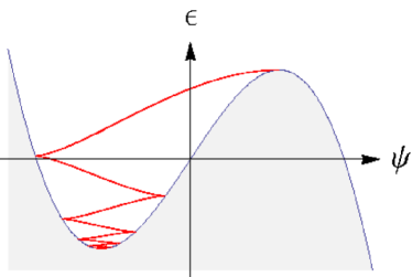
This differential equation has to be solved with initial condition , and integrated with the proper sign back and forth between the turning points until the integration ends at . A typical solution is depicted in Fig. 3.
In scaled units Eq. (88) takes the form
| (116) |
where the integral follows the -path back and forth between the turning points. Since the differential equation (114) depends on and only in the combination , we put
| (117) |
where
| (118) |
The function determines the correction of the exponential factor of the rate for arbitrary damping strength in the range of bias currents close to the critical current.
From Eq. (113), we obtain
| (119) |
while Eq. (100) gives for
| (120) |
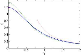
where we have made use of Eq. (115). In between these limiting results, the function needs to be determined numerically. A list of data points is provided in Table 1, and the function is depicted in Fig. 4 together with the findings of previous works.Ankerhold2 ; Sukhorukov This should facilitate the comparison with experimental results.
| 0 | 0.025 | 0.05 | 0.075 | 0.1 | 0.125 | 0.15 | 0.175 | |
|---|---|---|---|---|---|---|---|---|
| 1.188 | 1.185 | 1.179 | 1.169 | 1.157 | 1.142 | 1.125 | 1.107 |
| 0.2 | 0.225 | 0.25 | 0.5 | 0.75 | 1.0 | 1.5 | 2.0 | |
| 1.087 | 1.066 | 1.043 | 0.797 | 0.574 | 0.409 | 0.218 | 0.129 |
V.5 Conclusions
We have presented a theory for a Josephson junction detecting non-Gaussian fluctuations by means of the noise driven escape out of the zero-voltage state of the junction. It has been assumed that the device is operated in a regime where the barrier of the washboard potential is overcome by activated processes. This is always the case if the temperature is not too low and/or the junction capacitance is not too small. The study was based on the theory of irreversible processes and fluctuations developed by Onsager and MachlupOnsager and Grabert, Graham, and Green.GG ; GGG An extension of the method to account for non-Gaussian fluctuations was outlined.else In this approach the random motion of the system is described in terms of the state variables and the conjugate forces. The force conjugate to the electric charge , which appears naturally in this approach, plays a role similar to the counting field introduced in the more recent approaches to determine the full counting statistics of electronic devices.reviews
A nonlinear noise generating element in series with the Josephson detector modifies the rate of escape out of the zero-voltage state. The main effect comes from the second noise cumulant . However, this Gaussian part of the noise is detected by the Josephson junction in the same way as Johnson-Nyquist noise. Therefore, as was shown explicitly, the second noise cumulant can be described in terms of an effective temperature . Deviations from the accordingly modified Arrhenius law are thus due to higher order noise cumulants. The fluctuations causing the escape from the metastable well lead to fluctuations of the voltage across the Josephson junction. It has been shown that these voltage fluctuations are small compared to , which implies that the dimensionless random force causing these fluctuations is always small compared to 1. Since the order noise cumulant gives rise to terms of order , deviations from the modified Arrhenius law essentially only arise from the third noise cumulant , and these corrections are typically small. However, the third cumulant is odd under time reversal and the sign of the effect depends on the direction of the bias current. Comparing rates for pulses tilting the potential to the right and the left, respectively, the correction can be extracted.Pekola ; Pothier A Josephson junction threshold detector operating in the regime of noise activated escape thus can measure the third cumulant, the skewness of the noise, only. Another effect of the fluctuations of the voltage is a feedback of the Josephson detector on the noise generating device as described by the effective third noise cumulant defined in Eq. (73).
The modification of the rate exponent due to the skewness of the noise has been determined for arbitrary damping strength of the Josephson junction detector. Thereby, the theory developed goes considerably beyond the results of previous works,Ankerhold2 ; Sukhorukov that were restricted to limiting values of the damping strength or based on approximations. Explicit results where given for the case when the bias current is close to the critical current, which implies that the relevant part of the washboard potential can be described by a cubic potential. The effect of the skewness of the noise on the rate is, however, larger for smaller values of the bias current. Experimentally, the range of relevant bias currents can be influenced by the form of the applied current pulses. The theory presented here can readily also be evaluated for the exact form of the washboard potential allowing for results for any value of the bias current and all damping strengths.
To be explicit, we have presented the theory using the example of a normal state tunnel junction as noise generating device. However, the theory readily also applies to other noise generating elements, provided the correlation time of the noise is much smaller than the period of plasma oscillations of the detector. Finally, in this article, only the exponential factor of the rate has been determined. The corrections due to the skewness of the noise were found to be rather small, and they need sophisticated experimental techniques to be detected reliably. Corrections to the pre-exponential factor of the same order of magnitude are entirely negligible, so that safely the prefactor of the standard Gaussian noise theory can be employed.
Acknowledgements.
This work was carried out in the summer of 2007 during a sabbatical visit to CEA-Saclay. The warm hospitality of the Quantronics group and the enlightening discussions with the group members, in particular with D. Estève and H. Pothier, are gratefully acknowledged. The author also wishes to thank J. Ankerhold and J. Pekola for a number of interesting discussions, as well as D. Bercioux for discussions and providing the figures. Financial support was allocated by the European NanoSci-ERA Programme.Appendix A Validity of Nearly Gaussian Approximation
In this appendix we investigate the range of validity of the nearly Gaussian approximation used in Sec. IV. Since the leading order term of the most probable escape path is the time reversed relaxation path , the order of magnitude of the phase velocity during escape coincides with that during relaxation.
Let us first consider the case of weak damping. The trajectory starts with vanishing phase velocity at the barrier top. The largest kinetic energy arises when the potential minimum is reached for the first time. For weak damping the kinetic energy then almost equals the potential energy difference . Accordingly, the voltage satisfies
| (121) |
As damping increases the phase velocity and, accordingly, the maximal voltage across the Josephson junction decreases, so that will never exceed the estimate (121) in the entire range of parameters.
The plasma frequency of the Josephson junction at finite bias current
| (122) |
is the frequency of small undamped oscillations about the minimum of the potential (25). For , which is the case for , Eqs. (25) - (28) yield for the barrier height (39) of the potential
| (123) |
This can be combined with Eq. (122) to give
| (124) |
The bound (121) for the size of the fluctuations of may thus be written as
| (125) |
In the region of thermally activated escaperemark5 one has . In view of Eq. (125) this implies
| (126) |
so that is a small dimensionless parameter along the most probable escape path.
Now, the leading order contribution to the force causing the escape is determined by Eq. (65), entailing the estimate
| (127) |
which combines with the inequality (126) to give
| (128) |
This shows that an expansion of the Hamiltonian in terms of , as done in Eq. (45), is indeed justified. The terms of third order in are then small, so that and describe in fact small corrections to and , respectively.
Because of the weak effects of non-Gaussian statistics, the correction to the exponent of the rate is also small. From Eqs. (55) and (91), we find
| (129) |
For we can insert Eqs. (117) and (123). Using Eq. (28), we then find
| (130) |
Hence, the effect of the skewness of the noise vanishes proportional to as the bias current approaches . The ratio can be seen as a product of three factors
| (131) |
where we have made use of Eq. (122). Now, in the regime of activated decay the first factor is very small, while the last factor is of order 1 for weak to moderate damping. Hence, one needs a large factor to get observable effects from the skewness of the noise. Since is proportional to , this means large , in particular, , so that the estimate (74) for applies. To minimize the reduction of via the feedback effects described by Eq. (74), one needs to choose a bias resistor well below . Then the factor
| (132) |
This means that the current should be large compared to and thus needs to be largely compensated by a current in the opposite direction to keep the junction biasing current (48) below . Experimentally, this compensation problem is addressed by employing more sophisticated set-ups.Pekola ; Pothier
Appendix B Evaluation of Action of Escape Path
In this Appendix we evaluate the expressions (71) and (IV.3) for the action of the escape path in the nearly Gaussian approximation. Inserting the result (65) for , one obtains from (71)
| (133) | |||||
Now, vanishes at the integration boundaries and coincides there with and , respectively, since . Accordingly, Eq. (133) yields
| (134) |
which gives the exponential factor (55) of the escape rate.
After expressing in terms of and putting
| (135) |
we obtain from Eq. (IV.3) for the leading order non-Gaussian part of the action
The integral in the first line gives after partial integration
| (137) |
In this expression we can eliminate the second order derivatives and by means of the equations of motion (66) and (IV.2). Taking the definition (135) into account, we get
| (138) | |||||
This result can now be inserted into (B). After a partial integration of the term and a further partial integration along the lines , one obtains
From Eqs. (68) and (69), we see that
Now, under the integral , so that can be replaced by
| (141) |
where
| (142) |
Since the action (B) depends on only, is is natural to make the ansatz
| (143) |
From Eq. (135) and the equations of motion (66) and (IV.2) one then finds
| (144) |
Using Eqs. (68) and (69), the right hand side may be written as
| (145) |
where again the cumulants appear only in the combination (142).
We can now employ the evolution equation (144) to express the term proportional to in the action (B) in favor of terms with a purely polynomial dependence on . Using also Eqs. (141), (143), and (145), we find
| (146) | |||||
After partial integrations along the lines , , and , this simplifies to read
| (147) | |||||
Comparing the form of the evolution equation (144) with the one satisfied by , namely Eq. (58) for , we are led to the ansatz
| (148) |
Inserting this into Eq. (144) and using the evolution equation for as well as Eq. (145), we find that obeys the differential equation
| (149) |
which is satisfied, provided
| (150) |
When the ansatz (148) is plugged into (147), we obtain a term proportional to , which under the integral can be replaced by . Accordingly, we find
| (151) | |||||
Finally, in the integrand, the expression between squared brackets can be transformed by means of Eq. (150) to yield for the compact result
| (152) |
References
- (1) L. D. Landau and E. M. Lifshitz, Statistical Physics, (Pergamon, Oxford, 1975) Chapter XII.
- (2) L. S. Levitov and G. B. Lesovik, JETP Lett. 55, 555 (1992); L. S. Levitov, H. B. Lee, and G. B. Lesovik, J. Math. Phys. (N.Y.) 37, 4845 (1996).
- (3) For recent reviews see Y. M. Blanter and M. Büttiker, Phys. Rep. 336, 1 (2000) and articles in Quantum Noise in Mesoscopic Physics, edited by Yu. V. Nazarov, NATO Science Series in Mathematics, Physics and Chemistry (Kluwer, Dordrecht, 2003).
- (4) W. Schottky, Ann. Phys. (Leipzig), 57, 541 (1918).
- (5) B. Reulet, J. Senzier, and D. E. Prober, Phys. Rev. Lett. 91, 196601 (2003).
- (6) T. Fujisawa, T. Hayashi, Y. Hirayama, H. D. Cheong, and Y. H. Jeong, Appl. Phys. Lett. 84, 2343 (2004).
- (7) Yu. Bomze, G. Gershon, D. Shovkun, L. S. Levitov, and M. Reznikov, Phys. Rev. Lett. 95, 176601 (2005).
- (8) S. Gustavsson, R. Leturcq, B. Simovič, R. Schleser, T. Ihn, P. Studerus, K. Ensslin, D. C. Driscoll, and A. C. Gossard, Phys. Rev. Lett. 96, 076605 (2006).
- (9) A. V. Timofeev, M. Meschke, J. T. Peltonen, T. T. Heikkilä, and J. P. Pekola, Phys. Rev. Lett. 98, 207001 (2007).
- (10) B. Huard, H. Pothier, N. O. Birge, D. Estève, X. Waintal, and J. Ankerhold, Ann. Phys. (Leipzig) 16, 736 (2007).
- (11) J. Tobiska and Yu. V. Nazarov, Phys. Rev. Lett. 93, 106801 (2004).
- (12) J. P. Pekola, Phys. Rev. Lett. 93, 206601 (2004).
- (13) T. T. Heikkilä, P. Virtanen, G. Johansson, and F. K. Wilhelm, Phys. Rev. Lett. 93, 247005 (2004).
- (14) J. Ankerhold and H. Grabert, Phys. Rev. Lett. 95, 186601 (2005).
- (15) V. Brosco, R. Fazio, F. W. J. Hekking and J. P. Pekola, Phys. Rev. B 74, 024524 (2006).
- (16) J. Ankerhold, Phys. Rev. Lett. 98, 036601 (2007).
- (17) E. V. Sukhorukov and A. N. Jordan, Phys. Rev. Lett. 98, 136803 (2007).
- (18) F. Taddei and F. W. J. Hekking (unpublished).
- (19) L. Onsager and S. Machlup, Phys. Rev. 91, 1505 (1953); 91, 1512 (1953).
- (20) H. Grabert and M. S. Green, Phys. Rev. A 19, 1747 (1979).
- (21) H. Grabert, R. Graham, and M. S. Green, Phys. Rev. A 21, 2136 (1980).
- (22) A. Einstein, Ann. Phys. (Leipzig) 17, 459 (1905).
- (23) L. Onsager, Phys. Rev. 37, 405 (1931); 38, 2265 (1931).
- (24) State-dependent transport coefficients give rise to multiplicative noise and imply, for instance, differences between deterministic and average drift. Also the Riemannian curvature of state space needs to be accounted for. The full complexity of the problem is treated in the literatureGG ; GGG .
- (25) The relations from Refs. GG, ; GGG, have been specialized to a system with state-independent transport coefficients in contact with a heat bath.
- (26) M. Ivanchenko and L. A. Zil’berman, JETP Lett. 8, 113 (1968); V. Ambegaokar and B. I. Halperin, Phys. Rev. Lett. 22, 1364 (1969); T. A. Fulton and L. N. Dunkleberger, Phys. Rev. B 9, 4760 (1974).
- (27) B. D. Josephson, Rev. Mod. Phys. 46 251 (1974); A. Barone and G. Paterno Physics and Applications of the Josephson Effect (Wiley, New York, 1982).
- (28) For a review see M. H. Devoret, D. Estève, C. Urbina, J. Martinis, A. Cleland, and J. Clarke in Quantum Tunnelling in Condensed Media, edited by Yu. Kagan and A. J. Leggett (Elsevier, Amsterdam, 1992).
- (29) In fact, there is a one parameter family of solutions shifted relative to each other in time. This gives rise to a zero mode in the spectrum of fluctuations about the minimal action trajectory. Since in this work we restrict ourselves to the exponential factor of the rate expression, the fluctuation spectrum will not be addressed. The solution can be fixed by requiring in addition, e.g., for and .
- (30) See, for example, L. S. Schulman, Techniques and Applications of Path Integrals (Wiley, New York, 1981); P. Hänggi, P. Talkner, and M. Borkovec, Rev. Mod. Phys. 62, 251 (1990); U. Weiss,Quantum Dissipative Systems (World Scientific, Singapore, 1999).
- (31) A general account of the theory of irreversible processes and non-Gaussian fluctuations in terms of thermodynamically conjugate variables will be presented elsewhere.
- (32) Experimentally, the component is often eliminated with the help of an additional branch, see Refs. Pekola, ; Pothier, . However, since is an independently controlled current, the same range of parameters is accessible.
- (33) B. Huard, Ann. Phys. (Paris) 31, No. 4-5 (2006).
- (34) Experimentally, this region can be chosen even at low temperatures by making the junction capacitance sufficiently large, in case of need by means of a parallel shunt capacitor.