Belief Propagation and Loop Series on Planar Graphs

Abstract

We discuss a generic model of Bayesian inference with binary variables defined on edges of a planar graph. The Loop Calculus approach of [1, 2] is used to evaluate the resulting series expansion for the partition function. We show that, for planar graphs, truncating the series at single-connected loops reduces, via a map reminiscent of the Fisher transformation [3], to evaluating the partition function of the dimer matching model on an auxiliary planar graph. Thus, the truncated series can be easily re-summed, using the Pfaffian formula of Kasteleyn [4]. This allows to identify a big class of computationally tractable planar models reducible to a dimer model via the Belief Propagation (gauge) transformation. The Pfaffian representation can also be extended to the full Loop Series, in which case the expansion becomes a sum of Pfaffian contributions, each associated with dimer matchings on an extension to a subgraph of the original graph. Algorithmic consequences of the Pfaffian representation, as well as relations to quantum and non-planar models, are discussed.

1 Introduction

Bayesian Inference can be seen both as a sub-field of Information Theory and of general Statistical Inference [5]. A typical problem in this field is: given observed noisy data and known statistical model of a noisy communication channel (transition probability), as well as a prior distribution for the input (a pre-image), find the most likely pre-image, or compute the a posteriori marginal probability for some part of the pre-image.

This field is also deeply related to Combinatorial Optimization, which is a branch of optimization in Computer Science, related to operations research, algorithm theory and complexity theory [6]. A typical problem in Combinatorial Optimization is: solve, approximate or count (exactly or approximately) instances of problems by exploring the exponentially large space of solutions. In many emerging applications (in magnetic and optical recording, micro-fabrication, chip design, computer vision, network routing and logistics), the data are structured in a two-dimensional grid (array). Moreover, data associated with an element of the grid are often binary and correlations imposed by the problem are local, so that only nearest neighbors on the grid are correlated. Such problems are typically stated in terms of binary statistical models on planar graphs.

In this paper, we discuss a generic problem of Bayesian inference defined on a planar graph. We focus on the problem of weighted counting, or (from the perspective of statistical physics) we aim to calculate the partition function of an underlying statistical model. As the seminal work of Onsager [7] on the two-dimensional Ising model and its combinatorial interpretation by Kac and Ward [8] have shown, the planarity constraint dramatically simplifies statistical calculations. By contrast, three-dimensional statistical models are much more challenging, and no exact results are known.

Building on the work of physicists, specifically on results of Fisher [3, 9] and Kasteleyn [4, 10], Barahona [11] has shown that calculating the partition function of the spin glass Ising model on an arbitrary planar graph is easy, as the number of operations required to evaluate the partition function scales algebraically, $O(N^{3})$, with the size of the system. To prove this, the partition function of the spin-glass Ising model was reduced to a dimer model on an auxiliary graph, and the partition function was expressed as the Pfaffian of a skew-symmetric matrix defined on the graph. The polynomial algorithm was later used in simulations of spin glasses [12]. However, Barahona also added a grain of salt to the exciting positive result, showing that generic planar binary problem is difficult [11, 13]. Specifically, evaluating two-dimensional spin glass Ising model in a magnetic field is NP-hard, i.e. it is a task of likely exponential complexity.

When an exact computational algorithm of polynomial complexity is not available, efficient approximations become relevant. Typically, the approximation is built around a tractable case. One such approximate algorithm built around the Fisher-Kasteleyn Pfaffian formula was recently suggested by Globerson and Jaakkola in [14]. Although this approximation (coined “planar-graph decomposition”) gives a provable upper bound for the partition function for some special graphical models, it constitutes just heuristics, i.e. it suffers from lack of error-control and the inability of gradual error-reduction.

Controlling errors in approximate evaluations of the partition function of a graphical model is generally difficult. However, one recent approach, developed by two of us and called Loop Calculus [1, 2], offers a new method. Loop Calculus allows to express explicitly the partition function of a general statistical inference problem via an expansion (the Loop Series), where each term is explicitly expressed via a solution of the Belief Propagation [15, 16, 17], or Bethe-Peierls [18, 19, 20] (BP) equations. This brought new significance to the BP concept, which previously was seen as just heuristics.

The BP equations are tractable for any graph; generally, the number of terms in the Loop Series is exponentially large, so direct re-summation is not feasible. However, since any individual term in the series can be evaluated explicitly (once the BP solution is known), the Loop Series representation offers a possibility for correcting the bare BP approximation perturbatively, accounting for loop contributions one after another sequentially. This scheme was shown to work well in improving BP decoding of Low-Density Parity Check codes in the error-floor regime, where the number of important loop contributions to the Loop Series is (experimentally) small, and the most important loop contributions (comparable by absolute value to the bare BP one) have a simple, single-connected structure [21, 22]. In spite of this progress, the question remained: what to do with other truly difficult cases when the number of important loop corrections is not small, and when the important corrections are not necessarily single-connected? In general, we still do not know how to answer these questions, while a partial answer for the important class of planar models is provided in this paper.

1.1 Brief Description of Our Results

In this manuscript we show that, for any graph (planar or not), the partial sum of the loop series over single-connected loops reduces to evaluation of the full partition function of an auxiliary dimer-matching model on an extended, regular degree-3 graph. Weights of dimers calculated on the extended graph are expressed explicitly via solution of the respective BP equations. The dimer weights can be positive or negative. In general, summing the single-connected partition is not tractable. However, in the planar case, it reduces (through manipulations reminiscent of the Fisher-Kasteleyn transformations) to a Pfaffian defined on the extended graph, which is also planar by construction. Thus, we find a big class of planar graphical models which are computationally tractable by reduction (via a BP/gauge transformation) to a loop series including only single-connected loops, and summable into a Pfaffian. Moreover, we find that the partition function of the entire Loop Series is generally reducible to a weighted Pfaffians series, where each higher-order Pfaffian is associated with a sum of dimer configurations on a modified subgraph of the original graph. Each term in the Pfaffian series is computationally tractable via the Belief Propagation solution on the original graph.

The material in the manuscript is organized as follows. A formal definition of the model is given in Section 1.2 and a brief description of Loop Calculus [1, 2] forms Section 1.3. Some introductory material on the graphical transformations is also given in A. Section 2 is devoted to re-summation of the single-connected loops in the Loop Series (we called it single connected partition). Section 2.1 introduces graphical transformation from the original graph ${\cal G}$ to the extended graph ${\cal G}_{e}$, reminiscent the Fisher transformation [3, 9]. This allows to restate the single-connected loop partition of the Loop Series on the original graph in terms of a sum over dimer configurations on the extended graph. Subsection 2.2 adapts the Kasteleyn transformation [4, 10] to our case, thus expressing the partition function of the single-connected series as a Pfaffian of a matrix defined on the extended graph. Section 3 describes a set of graphical models reducible under Belief Propagation gauge (transformation) to a Loop Series which is computationally tractable. Section 4 describes the representation of the Loop Series for planar graphs in terms of the Pfaffian Series, where each Pfaffian sums dimer matchings on a graph extended from a subgraph of ${\cal G}$, with the later correspondent to exclusion of an even set of vertices from ${\cal G}$. Grassmann representations, as well as fermionic models are discussed in Section 5: a general set of Grassmann models on super-spaces is given in Section 5.1, while Section 5.2 addresses the relation between binary models and integrable hierarchies. A brief list of future research topics is given in Section 6.

1.2 Vertex-function Model

We introduce an undirected graph ${\cal G}=({\cal V},{\cal E})$ consisting of vertices ${\cal V}=(a=1,\cdots,N)$ and edges ${\cal E}$. This study focuses mainly on planar graphs, like those emerging in communication or logistics networks connecting or relating nearest neighbors on a 2d mesh or terrain. However, the material discussed in the present and the following Subsections is general, and applies to any graph, planar or not. A binary variable, $\sigma_{ab}=\pm 1$, which we will also be calling a spin, is associated with any edge $(a,b)\in{\cal E}$. The graphical model is defined in terms of the probability function

$$p(\vec{\sigma})=Z^{-1}\prod_{a\in{\cal V}}f_{a}(\vec{\sigma}_{a}),$$ (1)

for a spin configuration $\vec{\sigma}\equiv\{\sigma_{ab}=\pm 1|\forall(a,b)\in{\cal E}\}$. In (1), $\vec{\sigma}_{a}=(\sigma_{ab}|\forall b,\mbox{ s.t. }(a,b)\in{\cal E})$ is the vector built from all edge variables associated with the given vertex $a$. $f_{a}$’s are positive and otherwise we will assume no restrictions on the factor functions. $Z$ is the normalization factor, the so-called partition function of the graphical model.

We refer to (1) as “vertex-function” models, according to statistical physics notation [18]. In the information theory, they are known as Forney-style graphical models [23, 24].

We will assume in the following that the degree of connectivity of any vertex in the graph is three. Note that this is not a restrictive condition, as the $n$-th order vertices, correspondent to $n$-spin interactions with $n>3$, can always be represented in terms of a product of triplet terms. Then the $n$-th degree vertex can be transformed into a planar graph consisting of degree three vertices. We discuss transformations to the triplets, in general but also on some examples (Ising Model and Parity Check Decoding of a linear code), in A.

1.3 Loop Calculus

Loop Calculus [1, 2] gives an explicit expression for $Z$ through the Loop Series:

$$Z=Z_{0}\cdot z,\,\,z\equiv\left(1+\sum_{\it C}\prod\limits_{a\in{\it C}}\mu_{a,\bar{a}_{\it C}}\right),\,\,\mu_{a,\bar{a}_{\it C}}\equiv\frac{\tilde{\mu}_{a,\bar{a}_{\it C}}}{\prod\limits_{b\in{\it C}}^{(a,b)\in{\it C}}\sqrt{1-m_{ab}({\it C})}}$$ (2)

$$m_{ab}=\sum_{\sigma_{ab}}\sigma_{ab}b_{ab}(\sigma_{ab}),\,\,\tilde{\mu}_{a,\bar{a}_{\it C}}=\sum_{\vec{\sigma}_{a}}\prod_{b\in\bar{a}_{\it C}}(\sigma_{ab}-m_{ab})b_{a}(\vec{\sigma}_{a}),$$ (3)

where ${\it C}$ can be any allowed generalized loop on the graph ${\cal G}$, i.e. ${\it C}$ is a subgraph of ${\cal G}$ which does not contain any vertices of degree one; $\bar{a}_{\it C}$ is a set of vertices of graph ${\cal G}$ which are also contained in the generalized loop ${\cal C}$ (by construction $\bar{a}$ consists of two or three elements); and $b_{a}(\vec{\sigma}_{a})$ and $b_{ab}(\sigma_{ab})$ are beliefs associated with vertex $a$ and edge $(ab)$. The beliefs are defined via message variables $\eta_{ab}\neq\eta_{ba}$

$$\forall\ (a,b)\in{\cal E}:\quad b_{ab}(\sigma_{ab})=\frac{\exp\left((\eta_{ab}+\eta_{ba})\sigma_{ab}\right)}{2\cosh\left(\eta_{ab}+\eta_{ba}\right)},$$ (4)

$$\forall\ a\in{\cal V}:\quad b_{a}(\vec{\sigma}_{a})=\frac{f_{a}(\vec{\sigma}_{a})\exp\left(\sum_{b}^{(a,b)\in{\cal E}}\eta_{ab}\sigma_{ab}\right)}{\sum_{\vec{\sigma}_{a}}f_{a}(\vec{\sigma}_{a})\exp\left(\sum_{c}^{(a,c)\in{\cal E}}\eta_{ac}\sigma_{ac}\right)},$$ (5)

solving the following system of the Belief Propagation (BP) equations

$$\!\!\!\!\!\!\!\!\!\!\!\!\forall\ (a,b)\in{\cal E}:\quad\sum_{\vec{\sigma}_{a}}f_{a}(\vec{\sigma}_{a})\exp\left(\sum_{b}^{(a,b)\in{\cal E}}\eta_{ab}\sigma_{ab}\right)\left(\sigma_{ab}-\tanh\left(\eta_{ab}+\eta_{ba}\right)\right)=0.$$ (6)

The bare (BP) partition function $Z_{0}$ in Eq. (2) has the following expression in terms of the message variables:

$$Z_{0}=\frac{\prod_{a}\sum_{\vec{\sigma}_{a}\in{\cal V}}f_{a}\left(\vec{\sigma}_{a}\right)\exp\left(\sum_{(a,b)\in{\cal E}}\eta_{ab}\sigma_{ab}\right)}{\prod_{(a,b)\in{\cal E}}\left[2\cosh\left(\eta_{ab}+\eta_{ba}\right)\right]}.$$ (7)

BP equations (6) are interpreted as conditions on the gauge transformations, leaving the partition function of the model invariant. These equations may allow multiple solutions, related to each other via respective gauge transformations. The multiple solutions correspond to multiple extrema of the Bethe Free Energy and Loop Series can be constructed around any of the BP solutions.

2 Re-summation of the Single-connected Partition

In the following we will show how to re-sum a part of the Loop Series accounting for all the single-connected loops, i.e. subgraphs of ${\cal G}$ with all vertices of degree two

$$Z_{s}=Z_{0}\cdot z_{s},\quad z_{s}=1+\sum_{{\it C}\in{\cal G}}^{\forall a\in{\it C},\ |\delta(a)|_{\it C}=2}r_{\it C},$$ (8)

where $|\delta(a)|_{\it C}$ stands for the number of neighbors of $a$ within ${\it C}$. The evaluation will consist of the following two steps:

• Show that $z_{s}$ is equal to the partition function of the dimer-matching model on an auxiliary graph, ${\cal G}_{e}$. The graph will be constructed from the original ${\cal G}$ by a transformation reminiscent of the Fisher’s trick, introduced in [3, 9, 11] to streamline reduction of Ising model to the dimer-matching model;

• Use the Pfaffian formula of Kasteleyn [4, 10, 11] to reduce $z_{s}$ to a Pfaffian of a skew-symmetric matrix defined on ${\cal G}_{e}$. Note that complexity of the Pfaffian evaluation is $N^{3}$, where $N$ is the size of ${\cal G}$.

Note: while A) is valid for any graphical model, B) applies only to the planar case.

2.1 Transformation to Dimer Matching Problem

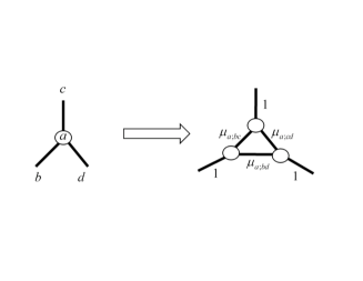
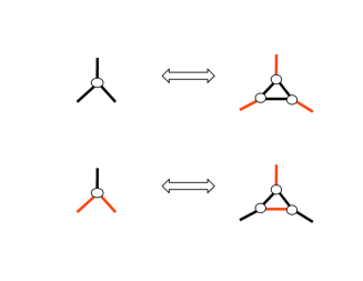
Figure 1: Left panel: Transformation from a vertex of ${\cal G}$ to respective three-vertex of the extended graph ${\cal G}_{e}$. Right panel: maps from the colorings of a vertex of ${\cal G}$ to coloring of the respective $3$-vertex of ${\cal G}_{e}$. Notice, that the coloring of the external edges of ${\cal G}_{e}$ are reversed in comparison with the coloring of original edges on ${\cal G}$.

Following the construction of Fisher [3, 9], we expand each vertex of ${\cal G}$ into a three-vertex of the extended graph ${\cal G}_{e}$, according to the scheme shown in the left panel of Figure 1. Consider a vertex $a$ of ${\cal G}$ and assume that $b,c,d$ are three neighbors of $a$ on ${\cal G}$. For each vertex $a$, there are three $\mu_{a;\bar{a}_{\it C}}$ contributions of degree two within a generalized loop ${\it C}$, i.e. with $|\delta\bar{a}_{\it C}|=2$, which can possibly contribute to the single-connected partition $r_{s}$: $\mu_{a;bc},\mu_{a;bd},\mu_{a;cd}$. We associate the three weights with internal edges of the respective three-vertex of ${\cal G}_{e}$, while the weights of all the external edges of the three-vertex are equal to unity. Then any coloring of the original graph, marking a single connected loop of ${\cal G}$, is in the one-to-one correspondence to a dimer-matching (which we also call coloring) of ${\cal G}_{e}$. The weights and coloring assignments are illustrated on an example at the left panel of Figure 1. An example of transformation mapping a single-connected-loop on ${\cal G}$ respective dimer on ${\cal G}_{e}$ is shown in Figure 2.

This map from the single-connected loops to dimers leads to the following representation for the single-connected partition $z_{s}$

$$z_{s}=\sum_{\vec{\pi}}\prod_{(a,b)\in{\cal G}_{e}}\left(\mu_{ab}\right)^{\pi_{ab}}\prod_{a}\delta\left(\sum_{b}^{(a,b)\in{\cal G}_{e}}\pi_{ab},1\right),$$ (9)

where the dimer-weights on ${\cal G}_{e}$ are defined according to the simple rules explained in the previous paragraph. One finds that the right hand side of (9) is nothing but the partition function of a dimer-matching problem on ${\cal G}_{e}$.

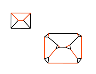
Figure 2: Example of ${\cal G}$ (upper left) to ${\cal G}_{e}$ (lower right) map. Single connected loop of ${\cal G}$ (shown in red) is in one-to-one correspondence with a valid dimer matching of ${\cal G}_{e}$, where dimers are also shown in red.

2.2 Pfaffian Expression for the Partition Function

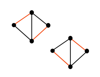
Figure 3: $\vec{p}$ orientation (left panel) and respective dimer (matching) configurations (right panel) correspondent to example of ${\cal G}_{e}$ described by Eq. (10).

Kasteleyn has shown in [4, 10] (see also [11]) that $z_{s}$ is equal to a Pfaffian (the square root of determinant) of a skew-symmetric matrix $\hat{A}=-\hat{A}^{t}$ of size $N_{a}\times N_{a}$, where $N_{a}$ is the number of vertices in ${\cal G}_{a}$. Each element of the matrix with $a>b$ (ordering is arbitrary, but it is fixed once and forever) is $A_{ab}=p_{ab}z_{ab}$, where $p_{ab}=\pm 1$. There are many possible choices of $\vec{p}=(\pi_{ab}=\pm 1|(a,b)\in{\cal G}_{e})$ which guarantee the Pfaffian relation: $z_{s}=\sqrt{\mbox{det}\hat{A}}$. A simple constructive way of choosing such a valid $\vec{p}$ is to relate it to orientation of edges in a directed version of ${\cal G}_{a}$, built according to the following “odd-face” rule: number of clockwise-oriented segments of any internal face of ${\cal G}_{e}$ should be negative. Example of a valid orientation is shown in Figure 2 and the respective expressions are

$$\!\!\!\!\!\!\!\!\!\!\!\!\!\!\!z_{s;{\it example}}=\mu_{12}\mu_{34}+\mu_{14}\mu_{23}=\sqrt{\mbox{Det}\hat{A}},\quad\hat{A}=\left(\begin{array}[]{cccc}0&-\mu_{12}&0&-\mu_{14}\\ \mu_{12}&0&\mu_{23}&-\mu_{24}\\ 0&-\mu_{23}&0&\mu_{34}\\ \mu_{14}&\mu_{24}&-\mu_{34}&0\end{array}\right)$$ (10)

Since calculating the determinant requires $\sim N_{a}^{3}$ operations, one finds that re-summation of all the single-connected loops in the Loop Series expression for the partition function of a planar graphical model can be done efficiently in $O(N_{a}^{3})$ steps.

3 Tractable Problems Reducible to Single-Connected Partition

In the case of a general vertex-function graphical model, the BP-gauge transformations, described by the set of BP equations (6), result in exact cancelation in the Loop Series of all the subgraphs containing at least one vertex of degree one within the subgraph. Thus, for the graph with all vertices of degree three, any vertex contributing a generalized loop (subgraph) should be of degree two or three within the subgraph. As shown in the previous Section, if one ignores generalized loops with vertices of degree three and the original graph is planar, the resulting sub-series (single-connected partition) is computationally tractable, i.e. the number of operations required to evaluate the single-connected partition is cubic in the system size (not exponential !).

In this Section we discuss the class of planar models whose Loop Series do not contain any generalized loops with vertices of degree three. According to Section 2, these models are tractable.

Indeed, it is known that BP Eqs. (6) have at least one solution for the set of messages $\{\eta\}$ on any graph and for any factor functions defined on the vertices of the graph. The aforementioned requirement for the generalized loop not to contain any vertex of degree three translates into the following set of additional equations

$$\!\!\!\!\!\!\!\!\forall\ a\in{\cal G}:\quad\sum_{\vec{\sigma}_{a}}f_{a}(\vec{\sigma}_{a})\prod_{b}^{(a,b)\in{\cal E}}\left(\exp\left(\eta_{ab}\sigma_{ab}\right)\left(\sigma_{ab}-\tanh\left(\eta_{ab}+\eta_{ba}\right)\right)\right)=0.$$ (11)

Considered together, the set of Eqs. (6,11) is overdefined, i.e. it cannot be solved in terms of $\eta$ variables for any values of the factor functions. However, if one allows flexibility in the factor functions, and, in fact, considers Eqs. (6,11) as a set of conditions on both the messages $\{\eta\}$ and the factor functions $\{f\}$, one arrives at a big set of possible solutions.

Therefore, Eqs. (6,11) define a big set of models reducible via BP transformations to a tractable Loop Series consisting only of single connected loops.

Moreover, the relations we established may be reversed. One may start from an arbitrary Loop Series consisting of only single connected loops, apply an arbitrary gauge transformation leaving the Loop Series invariant (these transformations are not necessarily of BP type), and arrive at a graphical model with some set of factor functions. At first sight, the resulting graphical model might not look tractable, but it actually is, by construction.

4 Loop Series as a Pfaffian Series

Let us notice that the general planar problem (e.g. spin glass in a magnetic field) is NP-hard [11], and it is thus not surprising that full re-summation does not allow expression in terms of a single Pfaffian (or a determinant).

On the other hand, we already found that a part of the Loop Series, specifically its single-connected partition, reduces to a computationally tractable Pfaffian. This suggests to represent the full Loop Series as a sum over terms, each representing a set of triplets (fully colored vertices of degree tree on ${\cal G}$):

$$z=\sum_{\Psi}z_{\Psi}\prod_{a\in\Psi}^{|\bar{a}|=3}\mu_{a;\bar{a}},$$ (12)

where $\Psi$ is either the empty set or any set of even nodes on ${\cal G}$; $\mu_{a;\bar{a}}=\mu_{a;bcd}$ are the weights from Eq. (2) associated with the triplet $(a;b,c,d)$, such that $(a,b),(a,c),(a,d)\in{\cal E}$; and $z_{\Psi}$ is the sum over all generalized loops (proper Loop Series colorings, i.e. subgraphs) of ${\cal G}$ such that all nodes of $\Psi$ are fully colored (all edges adjusted to the nodes belong to the generalized loop), while any other vertices of ${\cal G}$ are not colored or only partially colored. Thus, the first term in Eq. (12), where $\Psi$ is the empty set, represents the single-connected partition, $z_{s}$.

We show here that not only the first term in Eq. (12), associated with $\Psi=\varnothing$, but any term $z_{\Psi}$ in Eq. (12) is computationally tractable, being equal to a Pfaffian of a matrix defined on ${\cal G}_{e}$.

Indeed, it is straightforward to verify that the generalized loops associated with the given set of triplets (fully colored vertices) from the set $\Psi$ are in one-to-one correspondence with the set of dimer matchings on ${\cal G}_{e;\Psi}$, which is a subgraph of ${\cal G}_{e}$ with all $3$-vertices correspondent to $\Psi$, and external edges connected to the vertices, completely removed. Notice that some vertices of ${\cal G}_{e;\Psi}$ are of degree two. (These are vertices neighboring the removed triplets of $\Psi$.)

An example of a ${\cal G}_{e;\Psi}$ construction is given in Figure 4. One associates weights to the edges of ${\cal G}_{e;\Psi}$ in exactly the same way as for the single-connected partition: the weights of all the external edges of $3$-vertices of ${\cal G}_{e;\Psi}$ are equal to unity, while the internal edges are associated with the respective values $\mu_{a;bc}$, defined in Eq. (3).

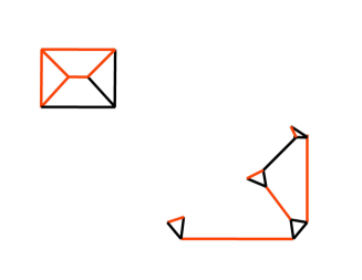
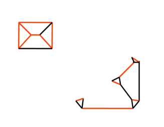
Figure 4: Two generalized loops (shown on the top) of an exemplary ${\cal G}$ correspondent to the same configuration of triplets $G$, $|G|=2$, and their respective dimer configurations on ${\cal G}_{e;\Psi}$ (shown on the bottom).

For any of ${\cal G}_{e;\Psi}$ one constructs the skew-symmetric $\hat{A}_{\Psi}$ matrix according to the Kasteleyn rule for the dimer-matching model described in Section 2.1. As before, the dimensionality of the matrix is $|{\cal G}_{e;\Psi}|\times|{\cal G}_{e;\Psi}|$ and each element of the matrix is the product of the respective dimer weight and orientation sign. Notice that the choice of signs for the elements of $\hat{A}_{\Psi}$ depends on the set of “excluded” triplets $\Psi$, and thus $\hat{A}_{\Psi}$ is not simply a minor of the original matrix $\hat{A}$, the one corresponding to the single-connected partition (without exclusion). Thus,

$$z_{\Psi}=\mbox{Pf}\left(\hat{A}_{\Psi}\right)=\sqrt{\mbox{Det}\left(\hat{A}_{\Psi}\right)}.$$ (13)

Eqs. (12,13) describe the Pfaffian series representation for the Loop Series of the planar problem.

5 Fermion Representation and Models

Any Pfaffian in Eq.(13) allows a compact representation in terms of Grassmann variables [25]. Indeed, let us associate a Grassmann (anti-commuting or fermionic) variable $\theta_{a}$ with each vertex of ${\cal G}_{e}$. The Grassmann variables satisfy

$$\forall(a,b)\in{\cal G}_{e}:\quad\theta_{a}\theta_{b}+\theta_{b}\theta_{a}=0,$$ (14)

and commute with ordinary $c$-numbers. One also introduces the Berezin integration rules over the Grassmann variables

$$\int d\theta=0,\quad\int\theta d\theta=1.$$ (15)

This translates into the following rule of Gaussian integration over the Grassmann variables:

$$\int\exp\left(-\frac{1}{2}\vec{\theta}^{t}\hat{A}\vec{\theta}\right)d\vec{\theta}=\mbox{Pf}(\hat{A})=\sqrt{\mbox{det}(\hat{A})},$$ (16)

where $\vec{\theta}$ is the vector of the Grassmann variables over the entire graph, $\vec{\theta}=\left(\theta_{i}|i\in{\cal G}_{a}\right)$ and $\hat{A}$ is an arbitrary skew-symmetric matrix on the graph. For example, applying this formula to the first term of the Pfaffian series (12) one derives

$$z_{\vec{0}}=\int\exp\left(-\frac{1}{2}\vec{\theta}^{t}\hat{A}\vec{\theta}\right)d\vec{\theta}.$$ (17)

In general, any term in the Pfaffian series of Eq. (12) can be represented as a Gaussian Grassmann integrable, however with different Gaussian kernels, not reducible simply to minors of $\hat{A}$.

5.1 Graphical Models on Super-Spaces

In this Subsection we first consider graphical models on spaces generalizing the $2$-point (binary) set to super-spaces containing commuting and anti-commuting parts. The models will be defined on arbitrary (non necessarily planar) graphs. Then, we return to the simple example (17) of pure dimer model with the Grassmann (anticommuting) variables defined on vertices of ${\cal G}_{e}$, to see that the model can be restated as the vertex-function Grassmann model on the original graph ${\cal G}$.

The general class of vertex-function models can be introduced as follows. For our graph, ${\cal G}$, consider a set of spaces $\{M_{a\alpha}|a\in\alpha\}$, i.e., we associate a space with any edge, $\alpha$, together with a vertex, $a$, that belongs to the edge. For simplicity we assume the spaces to be identical, i.e., $M_{a\alpha}\cong M$ for all $a\in\alpha$. The basic variables are $\sigma_{a\alpha}\in M_{a\alpha}$. We also introduce the notation (all products below are cartesian)

$$M_{a}=\prod_{\alpha\ni a}M_{a\alpha},\;\;M_{\alpha}=\prod_{a\in\alpha}M_{a\alpha},\;\;{\cal M}=\prod_{a\alpha}^{a\in\alpha}M_{a\alpha}=\prod_{a}M_{a}=\prod_{\alpha}M_{\alpha};\;\;$$ (18)

$$\vec{\sigma}_{a}\in M_{a},\;\;\vec{\sigma}_{\alpha}\in M_{\alpha},\;\;\vec{\sigma}\in{\cal M}.$$ (19)

Note that any $M_{\alpha}$ is a two-component cartesian product. The vertex-function model is determined by a set of vertex functions $f_{a}(\vec{\sigma}_{a})$ defined on $M_{a}$ and a set of integration measures $d\mu_{\alpha}(\vec{\sigma}_{\alpha})$ on $M_{\alpha}$. The model partition function is

$$Z=\int_{{\cal M}}\prod_{\alpha}d\mu_{\alpha}(\vec{\sigma}_{\alpha})\prod_{a}f_{a}(\vec{\sigma}_{a}).$$ (20)

For the particular case when measures have supports restricted to the diagonals $M\cong\Delta_{\alpha}\subset M_{\alpha}\cong M\times M$, i.e. ${\rm supp}\mu_{\alpha}\subset\Delta_{\alpha}$, we can consider the basic variables that belong to the diagonals. This corresponds to a more conventional formulation of the vertex-function models with the variables residing on edges. Note that the models introduced allow for loop-tower calculus [26], formulated in terms of fixing a proper gauge. The BP gauge fixing for a general vertex-function model described by Eq. (20) is nothing more than choosing basis sets in the vector spaces (maybe infinite-dimensional) of functions in $M_{a\alpha}$. A standard binary model, defined in Eq. (1), corresponds to the choice $M=\{0,1\}$ of the basic space to be a $2$-point set. Vertex models with $q$-ary alphabet, e.g. discussed in [26], are described by $M=\{0,1,\ldots,q-1\}$. Continuous models are obtained if $M$ is chosen to be a manifold of dimension $m$. The continuous case can be extended to the choice of $M$ to be a supermanifold $M$ of dimension $(m_{+},m_{-})$ that contains $m_{-}$ Grassmann (anticommuting) coordinates and whose substrate $\bar{M}\subset M$ is an $m_{+}$-dimensional manifold. Note that a manifold can be considered as a supermanifold with zero odd dimension $m_{-}=0$. In the remainder of this Subsection we will be dealing with an opposite case of the zero even dimension $m_{+}=0$, specifically with the purely Grassmann case of the $(0,1)$ supermanifold.

Eq. (17) is the partition function of a model stated in terms of Grassmann variables defined on the vertices of ${\cal G}_{e}$. The extended graph ${\cal G}_{e}$ is constructed from the original graph ${\cal G}$ so that a vertex of ${\cal G}$ extends into a triangle with three vertices of degree three (see the left panel of Figure 1). Therefore, the three Grassmann variables in (17) are associated with a vertex of ${\cal G}$. Then, Eq. (17) defined on ${\cal G}_{e}$ allows an obvious reformulation in the vertex-function form (20) on ${\cal G}$, where $\vec{\sigma}_{a}$ represents the three Grassmann variables that reside on the vertices of ${\cal G}_{e}$, obtained by expanding the vertex $a$ of the original graph. The dimer weights for the three edges of ${\cal G}_{e}$ associated with the extended vertex of ${\cal G}$ are encoded in the Gaussian function $f_{a}(\vec{\sigma}_{a})$. The dimer weight associated with an edge of ${\cal G}_{e}$ that represents and edge $\alpha$ of the original graph ${\cal G}$ is encoded in the integration measure $d\mu_{\alpha}(\vec{\sigma}_{\alpha})$.

Also notice that the vertex-function Grassmann model on a planar graph ${\cal G}$ can be restated as a model on the triangulated graph, dual to ${\cal G}$, with complex fermion (Grassmann) variables associated with the edges of the dual graph and functions associated with a face (elementary triangle) of the dual graph (Figure 7 illustrates the duality transformation). One interesting conclusion here is that the sequence of transformations discussed above leads us from a special binary model on a planar graph ${\cal G}$ to a Gaussian fermion (Grassmann) model on the dual graph, thus representing an instance of the disorder operator approach of Kadanoff-Ceva [27] developed originally for the Ising model on a square lattice.

5.2 Comments on Relation to Quantum Algorithms and Integrable Hierarchies

A mapping of a classical inference problem onto finding an expectation value in a corresponding quantum model takes on a natural interpretation as a quantum algorithm. This can be tried by using the theory of the infinite Kadomtsev-Petviashvilii (KP) hierarchy, specifically its fermionic formulation [28]. Consider $1D$ lattice fermions $\psi_{k},\psi_{k}^{*}$ with $k\in{\mathbb{Z}}$ and introduce the population $\widehat{n}_{k}=\psi_{k}^{*}\psi_{k}$ and shift operators $\widehat{H}_{k}=\sum_{j\in{\mathbb{Z}}}\psi_{k+j}^{*}\psi_{j}$. Let $|0\rangle$ denote the standard many-particle vacuum state where all single-fermion orbitals with $k\leq 0$ are occupied, and $|W\rangle$ is some uncorrelated (i.e. represented by a single Slater determinant) many-particle state, which is sufficiently close to $|0\rangle$. Introducing ${\bm{t}}=t_{1},t_{2},\ldots$, $\bar{{\bm{t}}}=\bar{t}_{0},\bar{t}_{1},\bar{t}_{2},\ldots$, and ${\bm{\xi}}=\ldots,\xi_{-1},\xi_{0},\xi_{1},\ldots$ we consider an expectation value

$$Z_{W}({\bm{t}},\bar{{\bm{t}}},{\bm{\xi}})=\langle 0|e^{\sum_{k>0}t_{k}\widehat{H}_{k}}e^{\sum_{k\in{\mathbb{Z}}}\xi_{k}\widehat{n}_{k}}e^{\sum_{k\leq 0}\bar{t}_{-k}\widehat{H}_{k}}|W\rangle$$ (21)

The approach is based on mapping the partition function of a classical inference problem on a graph onto a calculation of an expectation value represented by Eq. (21). We have established such a mapping for some simple Grassmannian models on planar graphs [29], where all the details on the suggested approach will be presented. Note that in the case ${\bm{\xi}}=0$ and $\bar{{\bm{t}}}=0$ the expectation value $Z_{W}({\bm{t}},0,0)=\tau_{W}({\bm{t}})$ is related to the $\tau$-function of the KP integrable hierarchy.

6 Future Challenges

We conclude with a brief and incomplete discussion of future challenges and opportunities raised by this study.

• We plan to extend the study looking at new approximate schemes for intractable planar problems. One new direction, suggested in Section 3, consists of exploring the vicinity of the computationally tractable models reducible via the BP-gauge transformation to the series of single-connected loops. It is also of great interest to explore the vicinity of integrable tractable models mentioned in 5.2.

• Perturbative exploration of a larger set of intractable non-planar problems which are close, in some sense, to planar problems, constitutes another interesting extension of the research. Here, one would aim to blend the aforementioned planar techniques with planar (or similar) decomposition techniques, e.g. these of the type discussed in [14].

• One important component of our analysis consisted in the Pfaffian re-summation of the single-connected loop (dimer) contributions, which is a special feature of the graph planarity. On the other hand, it is known that the planarity is equivalent to the graph being minor-excluded with respect to $K_{5}$ and $K_{3,3}$ subgraphs. Therefore, one wonders if there exists a generalization of the Pfaffian reduction to partition functions of models from other and/or broader graph-minor classes defined within the graph-minor theory [30]?Likewise, comparing with previous studies of the non-planar/non-spherical cases, based on the dimer approach [31, 32, 33].

• Extending the Loop Series analysis of the binary planar problem to the q-ary case seems feasible via the Loop Tower construction of [26]. This research should be of a special interest in the context of recently proposed polynomial quantum algorithm for calculating partition function of the Potts model [34]. Besides, recent progress [35, 36] shows that a Kasteleyn-type approach is extendable to a $q$-ary case, leading to the concept of “heaps of dimers”, and (in the continuum limit) to fascinating connections with special, highly symmetric complex surfaces, known as Harnack curves.

• One would also be interested to study how (and if) phase transitions in the disorder-averaged planar ensembles, e.g. analyzed in [37, 38, 39, 40, 41, 42, 43, 44, 45], are related to distribution of parameters characterizing computational tractability (complexity) of the models.

• In [46], the problem of finding all pseudo-codewords in a finite cycle code (corresponding to the type of graphical model discussed in this paper), was addressed by constructing a generating function known as graph zeta function [47]. The interesting fact discovered in [46] is that this generating function of pseudo-codewords has a determinant formulation, based on a discrete graph operator. Hence, one may anticipate an existence of yet uncovered relation between the graph zeta function and a Pfaffian-Loop resummation of related graphical models.

7 Acknowledgments

Research of M.C. and R.T. was carried out under the auspices of the National Nuclear Security Administration of the U.S. Department of Energy at Los Alamos National Laboratory under Contract No. DE C52-06NA25396, and specifically the LDRD Directed Research grant on Physics of Algorithms. M.C. also acknowledges support of the Weston Visiting Professorship program at the Weizmann Institute of Science, where he started to work on the manuscript. V.Y.C. acknowledges support through the start-up funds from Wayne State University.

Appendix A Graphical Transformations

In this Appendix we discuss graphical transformations reducing any binary problem to the vertex-function model described by Eq. (1), where all vertices are of degree three. Our main focus here is on the planar graphs, and on the graphical transformations preserving planarity. However some of the transformations and considerations discussed below apply to an arbitrary graph.

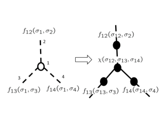
Figure 5: Transformation from binary variable on a vertex, $\sigma_{1}$, to set of variables, $\sigma_{12},\sigma_{13},\sigma_{14}$ on respective edges.

Often the original binary model is not represented in the vertex-function form. Some or all binary variables describing a problem may actually be assigned to vertices of a graph, then respective functions are associated with edges and not vertices. Obviously, one can also reformulate the model reducing it to the vertex (canonical for our purposes) form. The transformation is illustrated in Figure 5. Algebraic form of the transformation shown in the Figure reads, $\sum_{\sigma_{1}}f_{12}(\sigma_{1},\sigma_{2})f_{13}(\sigma_{1},\sigma_{3})f_{14}(\sigma_{1},\sigma_{4})=\sum_{\sigma_{12},\sigma_{13},\sigma_{14}}\chi(\sigma_{12},\sigma_{13},\sigma_{14})f_{12}(\sigma_{12},\sigma_{2})f_{13}(\sigma_{13},\sigma_{3})f_{14}(\sigma_{14},\sigma_{4})$, where $\chi(\sigma_{12},\sigma_{13},\sigma_{14})$ is the characteristic function equal to unity if all variables $\sigma_{12},\sigma_{13},\sigma_{14}$ are equal each other and equal to zero otherwise.

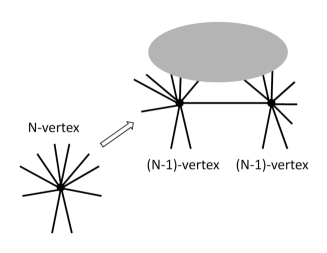
Figure 6: Transformation which allows reduction of an $N$-vertex to two $(N-1)$-vertices. It is assumed that (1) number of nodes in the gray area is not large, i.e. $O(N)$, (2) the new graph (on the right) is planar, (3) ordering (say clockwise) of the external nodes is preserved. The number of parameters characterizing the $N$-vertex is $2^{N}$ or smaller, thus the number of parameters characterizing the two $(N-1)$ vertices and vertices from the gray area is sufficient, i.e. $>2\cdot 2^{N-1}$, to parameterize the original vertex.

Next, let us notice that, given a vertex-function model (1) with the degree of connectivity higher than three, one can always perform a sequence of transformations reducing the degree of connectivity of all the nodes in the resulting graphical model to three. An elementary graphical transformation of the kind is illustrated in Figure 6. It is assumed that the transformation is applied sequentially to vertices of degree larger than three till none of these are left. The end result is that: (a) there are no vertices of degree larger than three left within the graph; (b) the increase in the total number of vertices is polynomial; (c) if the original graph is planar the resulting graph is also planar.

The set of transformations just described is general, and thus often inefficient, in the sense that knowing specific form of the factor functions one can practically always do a more efficient, customized and simpler reduction. Below we will illustrate this point on examples.

A.1 Ising Model

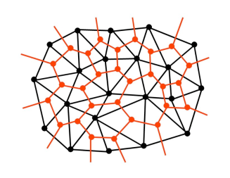
Figure 7: Planar triangulated graph (black) and its dual (red).

The spin glass Ising model is usually defined in terms of $\sigma_{i}=\pm 1$ variables associated with vertices of the graph

$$p({\bm{\sigma}})=Z^{-1}\exp\left(\sum_{(i,j)}J_{ij}\sigma_{i}\sigma_{j}\right),$$ (22)

where summation under the exponential on the r.h.s. goes over all edges of the graph, and $J_{ij}$ associated with an edge can be positive or negative. Obviously one can apply the vertex-to-edges transformation, explained in Figure 5, to restate the spin glass Ising model as a vertex-function model. However, in this case one can also do a simpler transformation to the dual graph. Let us consider a planar triangulated graph $\Gamma$ shown in black in Figure 7. All vertices of the respective dual graph, $\Gamma_{d}$, shown in red in Figure 7, have degree of connectivity three. We assume that the spin glass Ising model is defined on the planar triangulated graph $\Gamma$. Defining a new variable $\sigma_{ab}$ on an edge of $\Gamma_{d}$ as the product of two variables of the original graph $\sigma_{ab}\equiv\sigma_{i}\sigma_{j}$ connected by an edge $(i,j)$ of $\Gamma$ crossing the edge $(a,b$ of $\Gamma_{d}$, one finds that the sum on the r.h.s. of Eq. (22), rewritten in terms of the new variables, becomes, $\sum_{(a,b)\in\Gamma_{d}}J_{ab}\sigma_{ab}$. However, the new variables, $\sigma_{ab}$ are not independent, but rather related to each other via a set of local constraints, $\forall a\in\Gamma_{d}$: $\prod_{b}^{(a,b)\in\Gamma_{d}}\sigma_{ab}=1$. Then, Eq. (22) restated in terms of the new variables on the dual graph gets the following compact vertex-style form

$$p({\bm{\sigma}}_{d})=Z^{-1}\exp\left(\sum_{(a,b)\in\Gamma_{d}}J_{ab}\sigma_{ab}\right)\prod_{a\in\Gamma}\delta\left(\prod_{b}^{(a,b)\in\Gamma_{d}}\sigma_{ab},1\right).$$ (23)

One interesting observation is that the allowed configurations of ${\bm{\sigma}}_{d}\equiv\left(\sigma_{ab}|(a,b)\in\Gamma_{d}\right)$ on the dual graph correspond exactly to the single-connected loops on $\Gamma_{d}$, where the loops are built from the excited, $\sigma_{ab}=-1$, edges. Therefore, and in accordance with discussion of Section 2, calculation of the partition function for the spin glass Ising is reduced to evaluation of the respective Pfaffian, which is the task of a polynomial complexity. Notice also that adding a magnetic field (linear in $\sigma$) term in the expression under the exponent on the r.h.s. of Eq. (23) will raise the complexity level to exponential.

A.2 Parity-Check Based Error-Correction

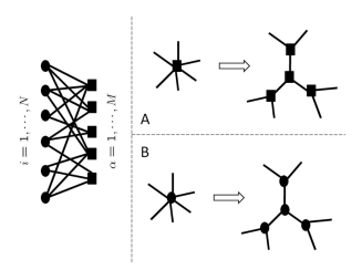
Figure 8: An illustrative example of a Tanner graph (left), as well as check-vertex (A) and bit-vertex transformations.

Consider a linear code with the code-book defined in terms of the bi-partite Tanner graph, $G=(V_{b},V_{c},{\cal E})$ consisting of $N=|V_{b}|$ bits and $M=|V_{c}|$ parity checks, and the set of edges ${\cal E}$ relating bits to checks and checks to bits. Then a message $\vec{\sigma}=(\sigma_{i}=0,1|i=1,\cdots N)$ is a codeword of the code if it satisfies all the parity checks, i.e. $\forall\alpha=1,\cdots M:\ \prod_{i}^{(i,\alpha)\in{\cal E}}\sigma_{i}=+1$. Assuming that all the codewords are equally probable originally, and that the white channel transform a bit $\sigma$ of the original codeword into the signal $x$ with the probability $p(x|\sigma)$, one finds that the probability for $\vec{\sigma}$ to be a codeword resulted in the measurement $\vec{x}$ is

$$p(\vec{\sigma}|\vec{x})=\frac{1}{Z}e^{\sum_{i\in V_{b}}\sigma_{i}h_{i}}\prod_{\alpha\in V_{c}}\delta\left(\prod_{i}^{(i,\alpha)\in{\cal E}}\sigma_{i},+1\right),\,\,\,h_{i}\equiv\frac{1}{2}\ln\frac{p(x_{i}|+1)}{p(x_{i}|-1)},$$ (24)

where, as usual, the partition function $Z$ is fixed by the normalization condition, $\sum_{\vec{\sigma}}p(\vec{\sigma}|\vec{x})=1$.

Eq. (24) represents an example of a mixed graphical model, with variables $\sigma_{i}$ defined on bit-vertices, the parity-check functions defined on check-vertices and the channel functions (carrying the dependencies on the log-likelihoods $h_{i}$) also associated with the bit-vertices. In this case transformation to the vertex-style model is done by direct application of the vertex-to-edges procedure of Figure 5 to all the bit-vertices of $G$. Then, the vertex-style version of Eq. (24) becomes

$$p(\vec{\sigma}|\vec{x})=Z^{-1}\prod_{\alpha\in V_{c}}f_{\alpha}(\vec{\sigma})\prod_{i\in V_{b}}f_{i}(\vec{\sigma}_{i}),$$ (25)

$$\forall i:\ \ \vec{\sigma}_{i}\equiv(\sigma_{i\alpha}=\pm 1|(i,\alpha)\in{\cal E}),$$ (26)

$$f_{i}(\vec{\sigma}_{i})=\left\{\begin{array}[]{cc}\exp(h_{i}\sigma_{i\alpha}),&\forall\alpha,\beta\mbox{ s.t. }(i,\alpha),(i,\beta)\in{\cal E}:\ \ \sigma_{i\alpha}=\sigma_{i\beta},\\ 0,&\mbox{otherwise}\end{array}\right.,$$ (29)

$$\forall\alpha:\ \ \vec{\sigma}_{\alpha}\equiv(\sigma_{i\alpha}|(i,\alpha)\in{\cal E}),\quad f_{\alpha}(\vec{\sigma}_{\alpha})=\delta\left(\prod_{i}^{(i,\alpha)\in{\cal E}}\sigma_{i\alpha},+1\right).$$ (30)

In general, degree of connectivity of bit-vertices and check-vertices may be arbitrary. Direct application of the general procedure explained above (see Figure 5 and discussion therein) allows to reduce all the higher-degree nodes to a larger set of nodes of degree three. However, a simpler dendro-reduction is possible both for the bit-vertices and check-vertices. The dendro trick (e.g. discussed in [48] for complexity reduction of a Linear Programming decoding of LDPC codes) is schematically illustrated in the two right panels of Figure 8, where respective algebraic relations are

$$\mbox{(A)}:\quad\delta\left(\prod_{i=1}^{6}\sigma_{i},+1\right)=$$ (31)

$$\sum_{\sigma_{12},\sigma_{34},\sigma_{56}=\pm 1}\delta(\sigma_{1}\sigma_{2}\sigma_{12},+1)\delta(\sigma_{3}\sigma_{4}\sigma_{34},+1)\delta(\sigma_{5}\sigma_{6}\sigma_{56},+1)\delta(\sigma_{12}\sigma_{34}\sigma_{56},+1),$$

$$\mbox{(B)}:\quad\delta\left(\sigma_{1},\cdots,\sigma_{6}\right)=$$ (32)

$$\sum_{\sigma_{12},\sigma_{34},\sigma_{56}=\pm 1}\delta(\sigma_{1},\sigma_{2},\sigma_{12})\delta(\sigma_{3},\sigma_{4},\sigma_{34})\delta(\sigma_{5},\sigma_{6},\sigma_{56})\delta(\sigma_{12},\sigma_{34},\sigma_{56}),$$

and $\delta(\sigma_{1},\cdots,\sigma_{6})$ is equal to unity if all arguments are the same, and it is zero otherwise.

Bibliography

Bibliography

- [1] Chertkov M and Chernyak V Y, Loop Calculus in Statistical Physics and Information Science, 2006 Phys. Rev. E 73 065102(R) [cond-mat/0601487]
- [2] Chertkov M and Chernyak V Y, Loop series for discrete statistical models on graphs, 2006 J. Stat. Mech. P06009 [cond-mat/0603189]
- [3] Fisher M E, Statistical Mechanics on a Plane Lattice, 1961 Phys. Rev 124 1664
- [4] Kasteleyn P W, The statistics of dimers on a lattice, 1961 Physics 27 1209
- [5] MacKay D, Information Theory, Inference, and Learning Algorithms, 2003 Cambridge Univ. Press
- [6] Papadimitriou C H and Steiglitz K, Combinatorial Optimization: Algorithms and Complexity, 1998 Dover
- [7] Onsager L, Crystal Statistics, 1944 Phys. Rev. 65 117
- [8] Kac M and Ward J C, A combinatorial solution of the Two-dimensional Ising Model, 1952 Phys. Rev. 88 1332
- [9] Fisher M E, On the dimer solution of planar Ising models, 1966 J. Math. Phys. 7 1776
- [10] Kasteleyn P W, Dimer Statistics and Phase Transitions, 1963 J. Math. Phys. 4 287
- [11] Barahona F, On the computational complexity of Ising spin glass models, 1982 J.Phys. A 15 3241
- [12] Saul L and Kardar M, Exact integer algorithm for the two-dimensional Ising spin glass, 1993 Phys. Rev. E 48 R3221
- [13] Jerrum M, Two-dimensional monomer-dimer systems are computationally intractable, 1987 J. Stat. Physics 48 121134
- [14] Globerson A and Jaakkola T, Approximate inference using planar graph decomposition, in Proceedings of Advances in Neural Information Processing Systems, 2006 20
- [15] Gallager R G, Low density parity check codes, 1963 MIT Press Cambridge MA
- [16] Gallager R G, Information Theory and Reliable Communication, 1968 J. Wiley New York
- [17] Pearl J, Probabilistic reasoning in intelligent systems: network of plausible inference, 1988 Kaufmann San Francisco
- [18] Baxter R J, Exactly Solved Models in Statistical Mechanics, 1982 Academic Press
- [19] Bethe H A, 1935 Proc. Roy. Soc. London A 150 552
- [20] Peierls R, Ising’s model of ferromagnetism, 1936 Proc. Camb. Phil. Soc. 32 477
- [21] Chertkov M and Chernyak V Y, Loop Calculus Helps to Improve Belief Propagation and Linear Programming Decodings of Low-Density-Parity-Check Codes, invited talk, 44th Allerton Conference 2006 [ arXiv:cs.IT/0609154]
- [22] Chertkov M, Reducing the Error Floor, invited talk at the Information Theory Workshop on “Frontiers in Coding” 2007 [http://arxiv.org/abs/0706.2926]
- [23] Forney G D, Codes on Graphs: Normal Realizations, 2001 IEEE IT 47 520-548
- [24] Loeliger H A, An Introduction to Factor Graphs, 2001 IEEE Signal Processing Magazine 28
- [25] Berezin F, Introduction to SuperAnalysis, 1987 Springer
- [26] Chernyak V and Chertkov M, Loop Calculus and Belief Propagation for q-ary Alphabet: Loop Tower, 2007 Proceedings of ISIT [cs.IT/0701086]
- [27] Kadanoff L P and Ceva H, Determination of an Operator Algebra for the Two-Dimensional Ising Model, 1971 Phys. Rev. B 3 3918
- [28] Sato M, Miwa T and Jimbo M 1977 Proc. Japan Acad. 53A 6; 1978 Publ. Res. Int. Math. Sci. 14 223; 1979 15 201 577 871; 1980 16 531
- [29] Teodorescu R, Chernyak V and Chertkov M, in preparation
- [30] Lovász L, Graph Minor Theory, 2005 Bulletin of the American Mathematical Society 43 75
- [31] Regge T and Zecchina R, Exact solution of the Ising model on group lattices of genus , 1996 J. Math. Phys. 37 2796-2814
- [32] Regge T and Zecchina R, Combinatorial and topological approach to the 3D Ising model, 2000 J. Phys. A: Math.Gen. 33 741
- [33] Galluccio A, Loebl M and Vondrak J, New algorithm for the Ising problem: Partition function for finite lattice graphs, 2000 Phys. Rev. Lett. 84 5924-5927
- [34] Aharonov D, Arad I, Eban E and Landau Z, Polynomial Quantum Algorithms for Additive approximations of the Potts model and other Points of the Tutte Plane, QIP 2007
- [35] Di Francesco P and Guitter E, Integrability of graph combinatorics via random walks and heaps of dimers, [arXiv:math/0506542v1]
- [36] Kenyon R and Okounkov A, Planar dimers and Harnack curves, [arXiv:math/0311062v2]
- [37] Sherrington D and Kirkpatrick S, 1975 Phys. Rev. Lett. 35
- [38] Dotsenko V S and Dotsenko V S, Critical behaviour of the phase transition in the 2D Ising Model with impurities, 1983 Advances in Physics 32 129-172
- [39] Honecker A, Picco M and Pujol P 2001 Phys. Rev. Lett. 87 047201
- [40] Amoruso C, Hartmann A K, Hastings M B and Moore M A 2006 Phys. Rev. Lett. 97 267202
- [41] Bhaseen B J, Caux J S, Kogan I I and Tsvelik A M 2001 Nucl.Phys. B 618 465
- [42] Efetov K, Supersymmetry in Disorder and Chaos, 1997 Cambridge University Press
- [43] Edwards S F and Anderson P W 1975 J. Phys. F 5 965
- [44] Fisher D S and Huse D A 1986 Phys. Rev. Lett. 56 1601
- [45] Mézard M, Parisi G and Virasoro M A, Spin Glass Theory and Beyond, 1987 World Scientific
- [46] Koetter R, Li W-C. W, Vontobel P O and Walker J L, Pseudo-codewords of cycle codes via zeta functions 2004 Proc. IEEE Inform. Theory Workshop p. 6
- [47] Horton M D, Stark H M and Terras A A, What are zeta functions of graphs and what are they good for? 2006 Contemporary Mathematics 415 173
- [48] Chertkov M and Stepanov M, Pseudo-codeword Landscape, 2007 Proc. of ISIT [cs.IT/0701084]