Adaptation dynamics of the quasispecies model

Abstract

We study the adaptation dynamics of an initially maladapted population evolving via the elementary processes of mutation and selection. The evolution occurs on rugged fitness landscapes which are defined on the multi-dimensional genotypic space and have many local peaks separated by low fitness valleys. We mainly focus on the Eigen’s model that describes the deterministic dynamics of an infinite number of self-replicating molecules. In the stationary state, for small mutation rates such a population forms a quasispecies which consists of the fittest genotype and its closely related mutants. The quasispecies dynamics on rugged fitness landscape follow a punctuated (or step-like) pattern in which a population jumps from a low fitness peak to a higher one, stays there for a considerable time before shifting the peak again and eventually reaches the global maximum of the fitness landscape. We calculate exactly several properties of this dynamical process within a simplified version of the quasispecies model.

I Introduction

Consider a maladapted population such as a bacterial colony in a glucose-limited environment, or a viral population in a vaccinated animal cell. In such harsh environments, the less fit members of the population are likely to perish and only the highly fit ones can survive to the next generation. In this manner, the fitness of the population increases with time and the initially maladapted population evolves to a well-adapted state. In the last century, there has been a concerted effort to put this verbal theory of Darwin Darwin (1859) on a solid quantitative footing by performing long-term experiments on microbial populations and studying theoretical models of biological evolution.

One of the questions in evolutionary biology concerns the mode of evolution. In the experiments on microbes, it is found that the fitness of the maladapted population can increase with time in either a smooth continuous manner Novella et al. (1995) or sudden jumps Elena and Lenski (2003). The latter mode is consistent with evolution on a fitness landscape defined on genotypic space with many local peaks separated by fitness valleys. On such a rugged fitness landscape, a low fitness population initially climbs a fitness peak until it encounters a local peak where it gets trapped since a better peak lies some mutational distance away. In a population of realistic size, it takes a finite time for an adaptive mutation to arise and the fitness stays constant during this time (stasis). Once some beneficial mutants become available, the fitness increases quickly as the population moves to a higher peak where it can again get stuck. Such dynamics alternating between stasis and rapid changes in fitness go on until the population reaches the global maximum.

This punctuated behavior of fitness is also seen in deterministic models that assume infinite population size. An example of such a step-like pattern for average fitness is shown in Fig. 1. A neat and unambiguous way of defining a step is by considering the fitness of the most populated genotype also shown in Fig. 1. Since large but finite populations evolve deterministically at short times Jain and Krug (2007a), it is worthwhile to study the punctuated evolution in models with infinite number of individuals. In this article, we will briefly describe some exact results concerning the dynamics of an infinitely large population on rugged fitness landscapes Jain and Krug (2005); Jain (2007a). We will find that the mechanism producing the step-like behavior is not due to “valley crossing” as in finite populations but when a fitter population “overtakes” the less fit one as described in the subsequent sections.

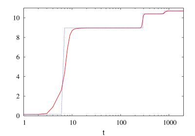
Figure 1: (Color online)Punctuated change in the average population fitness (dotted line) and the fitness of the most populated genotype (solid line) for an infinite population evolving on a maximally rugged fitness landscape. Here genome length $L=15$ and mutation probability $\mu=10^{-4}$.

II Quasispecies model and its steady state

We consider an infinitely large population reproducing asexually via the elementary processes of selection and mutation. Each individual in the population carries a binary string $\sigma=\{\sigma_{1},...,\sigma_{L}\}$ of length $L$ where $\sigma_{i}=0$ or $1$. The $2^{L}$ sequences are arranged on the multi-dimensional Hamming space. The information about the environment is encoded in fitness landscape defined as a map from the sequence space into the real numbers and is generated by associating a non-negative real number $W(\sigma)$ to each sequence $\sigma$. Fitness landscapes can be simple possessing some symmetry properties such as permutation invariance, or complex devoid of any such symmetries Gavrilets (2004); Jain and Krug (2007b). Fitness functions with single peak are an example of simple fitness landscapes while rugged landscapes with many hills and valleys belong to the latter class.

The average population fraction ${\cal X}(\sigma,t)$ with sequence $\sigma$ at time $t$ follows mutation-selection dynamics described by the following discrete time equation Eigen (1971); Jain and Krug (2007b)

$${\cal X}(\sigma,t+1)=\frac{\sum_{\sigma^{\prime}}p_{\sigma\leftarrow\sigma^{\prime}}W(\sigma^{\prime}){\cal X}(\sigma^{\prime},t)}{\sum_{\sigma^{\prime}}W(\sigma^{\prime}){\cal X}(\sigma^{\prime},t)}~{}.$$ (1)

The last two factors in the numerator of the above equation give the population fraction when a sequence $\sigma^{\prime}$ copies itself with replication probability $W(\sigma^{\prime})$ since fitness is defined as the average number of offspring produced per generation. After the reproduction process, point mutations are introduced independently at each locus of the sequence $\sigma^{\prime}$ with probability $\mu$ per generation. Thus, a sequence $\sigma$ is obtained via mutations in $\sigma^{\prime}$ with probability

$$p_{\sigma\leftarrow\sigma^{\prime}}=\mu^{d(\sigma,\sigma^{\prime})}(1-\mu)^{L-d(\sigma,\sigma^{\prime})}$$ (2)

where the Hamming distance $d(\sigma,\sigma^{\prime})$ is the number of point mutations in which the sequences $\sigma$ and $\sigma^{\prime}$ differ. The denominator of (1) is the average fitness of the population at time $t$ which ensures that the density ${\cal X}(\sigma,t)$ is conserved.

The stationary state of the quasispecies equation (1) has been studied extensively in the last two decades for various fitness landscapes. These numerical and analytical studies have shown that for most landscapes, there exists a critical mutation rate $\mu_{c}$ below which the population forms a quasispecies consisting of fittest genotype and its closely related mutants while above it, the population delocalises over the whole sequence space. This error threshold phenomenon can be easily demonstrated for a single peak fitness landscape defined as

$$W(\sigma)=W_{0}\delta_{\sigma,\sigma_{0}}+(1-\delta_{\sigma,\sigma_{0}})~{},~{}W_{0}>1$$ (3)

where $\sigma_{0}$ is the fittest sequence. In the limit $\mu\to 0,L\to\infty$ keeping $U=\mu L$ fixed, the frequency of the fittest sequence in the steady state of (1) is given by

$${\cal X}(\sigma_{0})=\frac{W_{0}e^{-U}-1}{W_{0}-1}$$ (4)

which is an acceptable solution provided $U\leq U_{c}=\ln W_{0}$. For $U>U_{c}$, selection is unable to counter the delocalising effects of mutation and the population can not be maintained at the fitness peak. For a discussion of error threshold phenomenon on other fitness landscapes and generalisations of the basic quasispecies equation (1), we refer the reader to Jain and Krug (2007b).

III Quasispecies dynamics on rugged fitness landscapes

We now turn our attention to the dynamical evolution of ${\cal X}(\sigma,t)$ on rugged fitness landscapes. We consider maximally rugged fitness landscapes for which the fitness $W(\sigma)$ is a random variable chosen independently from a common distribution. It is useful to introduce the unnormalised population defined as

$${\cal Z}(\sigma,t)={\cal X}(\sigma,t)\prod_{\tau=0}^{t-1}\sum_{\sigma^{\prime}}W(\sigma^{\prime}){\cal X}(\sigma^{\prime},t)$$ (5)

in terms of which the nonlinear evolution (1) reduces to the following linear iteration

$${\cal Z}(\sigma,t+1)=\sum_{\sigma^{{}^{\prime}}}p_{\sigma\leftarrow\sigma^{{}^{\prime}}}W(\sigma^{\prime}){\cal Z}(\sigma^{\prime},t)~{}.$$ (6)

Since at the beginning of the adaptation process the population finds itself at a low fitness genotype, we start with the initial condition ${\cal X}(\sigma,0)={\cal Z}(\sigma,0)=\delta_{\sigma,\sigma^{(0)}}$ where $\sigma^{(0)}$ is a randomly chosen sequence. For mutation probability $\mu\to 0$, after one iteration we have

$${\cal Z}(\sigma,1)\sim\mu^{d(\sigma,\sigma^{(0)})}W(\sigma^{(0)})~{}.$$ (7)

Thus in an infinite population model, each sequence gets populated in one generation obviating the need for “valley crossing” which is required for finite populations. Although an exact solution of (6) for $t>1$ is not available, it is possible to obtain several asymptotically exact results concerning the most populated genotype using a simplified version of the quasispecies dynamics. Numerical simulations of Krug and Karl (2003) showed that dynamical properties involving the most populated genotype are well described by a simplified model which approximates the population ${\cal Z}(\sigma,t)$ in (6) by

$${\cal Z}(\sigma,t)\sim\mu^{d(\sigma,\sigma^{(0)})}W^{t}(\sigma)~{},~{}t>1~{}.$$ (8)

This model ignores mutations once each sequence has been populated and allows the population at each sequence to grow with its own fitness. However, a recent perturbative analysis in the small parameter $\mu$ shows that this approximation holds for highly fit sequences and at short times Jain (2007a).

Writing $W(\sigma)=e^{F(\sigma)}$ and rescaling time by $|\ln\mu|$ in (8), we find that the logarithmic population $E(\sigma,t)$ obeys the following linear equation:

$$E(\sigma,t)=-d(\sigma,\sigma^{(0)})+F(\sigma)~{}t~{}.$$ (9)

The linear evolution of the (logarithmic) population of $2^{L}$ sequences for $L=4$ is shown in Fig. 2a. Since the initial population fraction given by (7) is same for all the sequences at constant Hamming distance $d(\sigma,\sigma^{(0)})$ from $\sigma^{(0)}$, ${L\choose d}$ lines are seen to emanate from the same intercept. However as the genotype with the largest slope (fitness) at constant intercept has the potential to become the most populated sequence, we arrive at the model in Fig. 2b in which $L+1$ genotypes are retained, each of whose fitness $F(k),k=0,...,L$ is an independent but non-identically distributed variable Krug and Karl (2003); Jain and Krug (2005).

Figure 2: (a) Evolutionary trajectories $E(\sigma,t)$ defined by (9) for $L=4$. The bold lines have the largest fitness amongst the ${L\choose k}$ fitnesses at distance $k$ from the origin. (b) Evolutionary race: The sequence at distance $3$ is the most populated sequence (winner) while the one at distance $2$ is a record (contender).

In a sequence $\{F(k)\}$ of random variables, a record is said to occur at $m$ if $F(m)>F(k)$ for all $k<m$. In Fig. 2b, the sequences at distance $k=0,2$ and $3$ from the initial sequence are records but the sequence at $k=2$ does not become a most populated genotype. In order to qualify as a jump, it is not sufficient to have a record fitness; the population should also be able to overtake the current winner in minimum time. Due to the overtaking time minimization constraint, the records and jumps have different statistical properties which we describe briefly in the next subsections.

III.1 Statistics of records

Although the record statistics for independent and identically distributed (i.i.d.) random variables is well studied, much less is known when the variables are not i.i.d.Nevzorov (2001). Here we have a situation in which $F(k)$ is a maximum of $\alpha_{k}={L\choose k}$ i.i.d. random variables. However, since the $k$th record fitness $F(k)$ is the largest amongst $\sum_{j=0}^{k}\alpha_{j}$ i.i.d. variables and there are $\alpha_{k}$ ways of choosing it, the probability $\tilde{P}_{k}$ that the $k$th fitness is a record is given by Jain and Krug (2005); Krug and Jain (2005)

$$\tilde{P}_{k}=\frac{{L\choose k}}{\sum_{j=0}^{k}{L\choose j}}\approx\frac{L-2k}{L-k}~{},~{}k<L/2~{}.$$ (10)

The meaning of the above distribution is intuitively clear: as it is easier to break records in the beginning, the probability to find a record is near unity for $k\ll L$ and it vanishes beyond $L/2$ because the global maximum typically occurs at this distance. The average number ${\cal{R}}$ of records can be obtained by simply integrating $\tilde{P}(k)$ over $k$ to yield ${\cal{R}}\approx(1-\ln 2)L$. It is also possible to find the typical spacing $\tilde{\Delta}(j)$ between the $j$th and $(j+1)$th record where we have labeled the last record (i.e. global maximum) as $j=1$. A straightforward calculation shows that the typical inter-record spacing falls as a power law given by Jain and Krug (2005)

$$\tilde{\Delta}(j)\approx\sqrt{\frac{L}{4\pi j}}\;\;,\;\;j\gg 1\;\;.$$ (11)

The above expression indicates that the spacing between the last few records (i.e $j\sim{\cal{O}}(1)$) is of order $\sqrt{L}$, while most of the records are crowded at the beginning which is consistent with the behavior of the record occurrence probability (10).

III.2 Statistics of jumps

The calculation of jump statistics Jain (2007a) is more involved than that of records because a jump event requires a minimization of the overtaking time. This constraint imposes a condition on the fitnesses of the squences that can possibly overtake the current leader in a time interval between $t$ and $t+dt$. The sequence at distance $k^{\prime}$ can overtake the $k$th one (with fitness $F$) at time $t$ if the fitness $F(k^{\prime})=(E(k,t)+k^{\prime})/t$ and at time $t+dt$, $dt/t\to 0$ if

$$F(k^{\prime})=\frac{E(k,t+dt)+k^{\prime}}{t+dt}=F+\frac{k^{\prime}-k}{t}-\frac{k^{\prime}-k}{t^{2}}dt+{\cal O}(dt^{2})~{}.$$

Then the total collision rate $W_{k^{\prime},k}(F,t)$ with which the $k$th sequence is overtaken by the $k^{\prime}$th one is given as

$$W_{k^{\prime},k}(F,t)\approx\frac{k^{\prime}-k}{t^{2}}~{}p_{k^{\prime}}\left(F+\frac{k^{\prime}-k}{t}\right)~{},~{}k^{\prime}>k~{}$$ (12)

where $p_{k}(F)$ is the distribution of the maximum of $\alpha_{k}$ i.i.d. random variables distributed according to $p(F)$ with support over the interval $\left[F_{\rm{min}},F_{\rm{max}}\right]$. Using this collision rate, we can write the probability ${\cal P}_{k^{\prime},k}(t)$ that the sequence at distance $k^{\prime}$ overtakes the $k$th one at time $t$ as

$${\cal P}_{k^{\prime},k}(t)=\int_{F_{\rm{min}}}^{F_{\rm{max}}}dF~{}W_{k^{\prime},k}(F,t)~{}P_{k}(F,t)$$ (13)

where the probability $P_{k}(F,t)$ that the $k$th sequence has the largest population at time $t$ is given by

$$P_{k}(F,t)=p_{k}(F)~{}\prod_{\begin{subarray}{c}j=0\\ j\neq k\end{subarray}}^{L}\int_{F_{\rm{min}}}^{F+\frac{j-k}{t}}dF^{\prime}~{}p_{j}(F^{\prime})~{}.$$ (14)

Note that unlike the records, the jump properties depend on the underlying distribution of the random variables. Below we present some results when the distribution $p(F)=e^{-F}$.

Integrating (13) over time, the probability distribution $P_{k^{\prime},k}$ that $k$th sequence is overtaken by $k^{\prime}$th sequence is obtained,

$$P_{k^{\prime},k}\approx\sqrt{\frac{L}{\pi k(L-k)}}~{}\left(\frac{k^{\prime}-k}{2k}\right)~{}e^{-\frac{L(k^{\prime}-k)^{2}}{4k(L-k)}}~{},~{}k<k^{\prime}<L/2~{}.$$ (15)

This form of the distribution implies that the overtaking sequence $k^{\prime}$ is located within ${\cal O}(\sqrt{k})$ distance of the overtaken sequence $k$. Thus the typical spacing between successive jumps for large $k$ is roughly constant and goes as $\sqrt{L}$ unlike in the case of records discussed in the last subsection. The jump distribution $P_{k}$ for a jump to occur at distance $k$ is obtained by integrating over $k^{\prime}$ and we have Jain (2007a)

$$P_{k}\approx\sqrt{\frac{L}{\pi k(L-k)}}~{}\theta_{H}\left(\frac{L}{2}-k\right)$$ (16)

where $\theta_{H}$ is the Heaviside step function which takes care of the fact that the record distribution (10) vanishes at distance $L/2$. Instead of integrating over time, by summing over the space variables $k,k^{\prime}$ in (13), the probability $P(t)$ that a jump occurs at time $t$ can be obtained and is given by Jain (2007a)

$$P(t)=\sqrt{\frac{L}{4\pi}}~{}\frac{1}{t^{2}}~{}\mathrm{sech}\left(\frac{1}{2t}\right)~{}.$$ (17)

The heavy tail distribution $P(t)\sim t^{-2}$ can be understood using a simple argument Krug and Karl (2003) and implies that mean overtaking time is infinite. Finally, by either summing $P_{k}$ over $k$ or integrating $P(t)$ over time, the total number of jumps ${\cal J}$ are found to be $\sqrt{L\pi}/2$ which is much smaller than the number of records ${\cal R}$.

IV Summary

In this article, we discussed the steady state and the dynamics of the quasispecies model which describes a self-replicating population evolving under mutation-selection dynamics. On rugged fitness landscapes, the population fitness increases in a punctuated fashion and we described several exact results concerning this mode of evolution. Our recent simulations indicate that the $1/t^{2}$ law in (17) for the deterministic populations also holds for finite stochastically evolving populations Jain (2007a). At present, we do not have an analytical understanding of the latter result but it should be possible to test this law in long-term experiments such as those of Elena and Lenski (2003) on E. Coli.

Acknowledgements: I am very grateful to Prof. J. Krug for introducing me to the area of theoretical evolutionary biology. I also thank the organisers of the Statphys conference at IIT, Guwahati for giving me an opportunity to present my work.

References

- Darwin (1859) C. Darwin, The origin of species by means of natural selection (John Murray, London, 1859).
- Novella et al. (1995) I. Novella, E. Duarte, S. Elena, A. Moya, E. Domingo, and J. Holland, Proc. Natl. Acad. Sci. USA 92, 5841 (1995).
- Elena and Lenski (2003) S. F. Elena and R. E. Lenski, Nat. Rev. Genet. 4, 457 (2003).
- Jain and Krug (2007a) K. Jain and J. Krug, Genetics 175, 1275 (2007a).
- Jain and Krug (2005) K. Jain and J. Krug, J. Stat. Mech.: Theor. Exp. p. P04008 (2005).
- Jain (2007a) K. Jain, Phys. Rev. E 76, 031922 (2007a).
- Gavrilets (2004) S. Gavrilets, Fitness landscapes and the origin of species (Princeton University Press, 2004).
- Jain and Krug (2007b) K. Jain and J. Krug, in Structural approaches to sequence evolution: Molecules, networks and populations, edited by U. Bastolla, M. Porto, H. Roman, and M. Vendruscolo (Springer, Berlin, 2007b), pp. 299–340, eprint arXiv:q-bio.PE/0508008.
- Eigen (1971) M. Eigen, Naturwissenchaften 58, 465 (1971).
- Krug and Karl (2003) J. Krug and C. Karl, Physica A 318, 137 (2003).
- Nevzorov (2001) V.B. Nevzorov, Records: Mathematical Theory (Providence, RI: American Mathematical Society, 2001).
- Krug and Jain (2005) J. Krug and K. Jain, Physica A 358, 1 (2005).