^(a) High Energy Accelerator Research Organization (KEK)
1-1 Oho, Tsukuba 305-0801, Japan

^(b) University of Tokyo, International Center for Elementary Particle Physics (ICEPP)
7-3-1 Hongo, Bunkyo-ku, Tokyo 113-0033, Japan

Abstract
In a class of new physics models, new physics sector is completely or partly hidden, namely, singlet under the Standard Model (SM) gauge group. Hidden fields included in such new physics models communicate with the Standard Model sector through higher dimensional operators. If a cutoff lies in the TeV range, such hidden fields can be produced at future colliders. We consider a scalar field as an example of the hidden fields. Collider phenomenology on this hidden scalar is similar to that of the SM Higgs boson, but there are several features quite different from those of the Higgs boson. We investigate productions of the hidden scalar at the International Linear Collider (ILC) and study the feasibility of its measurements, in particular, how well the ILC distinguishes the scalar from the Higgs boson, through realistic Monte Carlo simulations.

1 Introduction

In a class of new physics models, a new physics sector is completely or partly singlet under the Standard Model (SM) gauge group, SU(3)${}_{C}\times$SU(2)${}_{L}\times$U(1)_Y. Such a new physics sector, which we call “hidden sector” throughout this paper, includes some singlet fields. These hidden sector fields, in general, couple with the SM fields through higher dimensional operators. If the cutoff scale of the higher dimensional operators lies around the TeV scale, effects of the hidden fields are accessible at future colliders such as the Large Hadron Collider (LHC) and the International Linear Collider (ILC).

There have been several new physics models proposed that include hidden fields. The most familiar example would be the Kaluza-Klein (KK) modes of graviton in extra dimension scenarios [1] [2]. A singlet chiral superfield in the next to Minimal Supersymmetric Standard Model (MSSM) [3] is also a well-known example, which has interesting implications, in particular, on Higgs phenomenology in collider physics [4]. Another example is the supersymmetry breaking sector of the model proposed in Ref. [5], where a singlet scalar field couples with the SM fields through higher dimensional operators with a cutoff around $\Lambda=1-10$ TeV and its collider phenomenology at the LHC and ILC has been discussed. A very recently proposed scenario [6], “unparticle physics”, belongs to this class of models, whose phenomenological aspects have been intensively studied by many authors.

In this paper, we introduce a hidden scalar field and investigate the hidden scalar production at the ILC. We assume that the hidden scalar couples with only the SM gauge fields through higher dimensional operators suppressed by a TeV-scale cutoff. In this case, at the ILC, this hidden scalar can be produced through the similar process to the SM Higgs boson production and with the production cross sections comparable to the Higgs boson one. Thus, the hidden scalar production has interesting implications on the Higgs phenomenology. The crucial difference of the hidden scalar from the Higgs boson lies in that the hidden scalar has nothing to do with the electroweak symmetry breaking. This feature reflects the fact that the hidden scalar couples with mostly the transverse mode of the weak gauge bosons while the Higgs boson couples with mostly their longitudinal modes. The hidden scalar could be discovered at the LHC (together with the Higgs boson) and then, would be identified as a Higgs boson-like particle. It is an interesting issue how to distinguish the scalar irrelevant to the electroweak symmetry breaking from the relevant one (the Higgs boson). It would be challenging to tackle this issue with the LHC. In this paper, based on realistic Monte Carlo simulations, we study the feasibility of measurements for the hidden scalar productions and its couplings to the SM particles, and show how well the hidden scalar can be distinguished from the Higgs boson at the ILC.

This paper is organized as follows. In the next section, we introduce our theoretical framework and present formulas relevant to our studies. In Sec. 3, we show the results from our Monte Carlo simulations and demonstrate how accurately the ILC can measure the typical features of the scalar and distinguish it from the Higgs boson. The last section is devoted to summary and discussions.

2 Theoretical framework

In this paper, we introduce a real scalar field $\chi$ as a hidden field, which communicates with the SM sector through interactions of the form,

$${\cal L}_{\rm int}=\frac{c_{i}}{\Lambda^{d_{\rm SM}-3}}\chi\;{\cal O}_{\rm SM}^{i},$$ (1)

where $c_{i}$ is a dimensionless coefficient, $\Lambda$ is a cutoff scale, and ${\cal O}_{\rm SM}^{i}$ is an operator of the SM fields with mass dimension $d_{\rm SM}$. We consider the case that the cutoff, which is naturally characterized by a new physics scale, is around the TeV scale. As an example, it would be easy to imagine a model like the large extra-dimension models [1] whose fundamental scale is in the TeV range or a model with warped extra dimensions [2] where the effective cutoff scale is warped down to the TeV range from the 4-dimensional Planck scale. For a more concrete example, see Ref. [5]. In these models, the above effective interaction can be introduced at tree level.

The theoretical requirements for the SM operator ${\cal O}_{\rm SM}^{i}$ are that it should be a Lorentz scalar operator and be singlet under the SM gauge group. Although there are many possibilities for such operators, we assume that the hidden scalar couples with only the SM gauge bosons through the operators descried as follows:

$${\cal L}_{\rm int}=-\frac{1}{2}\sum_{A}\;c_{A}\;\frac{\chi}{\Lambda}\;{\rm tr}\left[{\cal F}_{A}^{\mu\nu}{\cal F}_{A\mu\nu}\right],$$ (2)

where $c_{A}$ is a dimensionless parameter, and ${\cal F}_{A}$’s ($A=1,2,3$) are the field strengths of the corresponding SM gauge groups, U(1)_Y, SU(2)_L, and SU(3)_C. After the electroweak symmetry breaking, Eq. (2) is rewritten as interactions between $\chi$ and gluons, photons, $Z$- and $W$-bosons.

$${\cal L}_{\rm int}= - \frac{c_{gg}}{4}\frac{\chi}{\Lambda}G^{a\mu\nu}G^{a}_{\mu\nu}-\frac{c_{WW}}{2}\frac{\chi}{\Lambda}W^{+\mu\nu}W^{-}_{\mu\nu}-\frac{c_{ZZ}}{4}\frac{\chi}{\Lambda}Z^{\mu\nu}Z_{\mu\nu}$$ (3)

$$- \frac{c_{\gamma\gamma}}{2}\frac{\chi}{\Lambda}F^{\mu\nu}F_{\mu\nu}-\frac{c_{Z\gamma}}{4}\frac{\chi}{\Lambda}Z^{\mu\nu}F_{\mu\nu},$$

where $G^{a\mu\nu}$, $W^{+\mu\nu}$, $Z^{\mu\nu}$ and $F^{\mu\nu}$ are the field strengths of gluon, $W$-boson, $Z$-boson and photon, respectively. The couplings $c_{gg}$ etc. can be described in terms of the original three couplings, $c_{1}$, $c_{2}$ and $c_{3}$, and the weak mixing angle $\theta_{w}$ as follows:

$$c_{gg} = c_{3},$$

$$c_{WW} = c_{2},$$

$$c_{ZZ} = c_{1}\sin^{2}\theta_{w}+c_{2}\cos^{2}\theta_{w},$$

$$c_{\gamma\gamma} = c_{1}\cos^{2}\theta_{w}+c_{2}\sin^{2}\theta_{w},$$

$$c_{Z\gamma} = (-c_{1}+c_{2})\sin\theta_{w}\cos\theta_{w}.$$ (4)

The hidden scalar can be produced at the ILC through these interactions. The dominant $\chi$ production process is the associated production, $e^{+}e^{-}\rightarrow\gamma^{*},Z^{*}\rightarrow Z\chi$ and $e^{+}e^{-}\rightarrow\gamma^{*},Z^{*}\rightarrow\gamma\chi$. First, let us consider the process $e^{+}e^{-}\rightarrow Z\chi$. The cross section is calculated as

$$\frac{d\sigma}{d\cos\theta}(e^{+}e^{-}\rightarrow Z\chi)=\frac{1}{68\pi s}\sqrt{\frac{E_{Z}^{2}-m_{Z}^{2}}{s}}$$ (5)

$$\times \left[\left(c_{ZZ}^{2}(g_{L}^{2}+g_{R}^{2})\left(\frac{s}{s-m_{Z}^{2}}\right)^{2}-c_{ZZ}c_{Z\gamma}(g_{L}+g_{R})e\left(\frac{s}{s-m_{Z}^{2}}\right)+c_{Z\gamma}^{2}e^{2}\right)\frac{E_{Z}^{2}}{\Lambda^{2}}(1+\cos^{2}\theta)\right.$$

$$+ \left.\left(c_{ZZ}^{2}(g_{L}^{2}+g_{R}^{2})\left(\frac{s}{s-m_{Z}^{2}}\right)^{2}-\sqrt{2}c_{ZZ}c_{Z\gamma}(g_{L}+g_{R})e\left(\frac{s}{s-m_{Z}^{2}}\right)+\frac{c_{Z\gamma}^{2}e^{2}}{2}\right)\frac{m_{Z}^{2}}{\Lambda^{2}}\sin^{2}\theta\right],$$

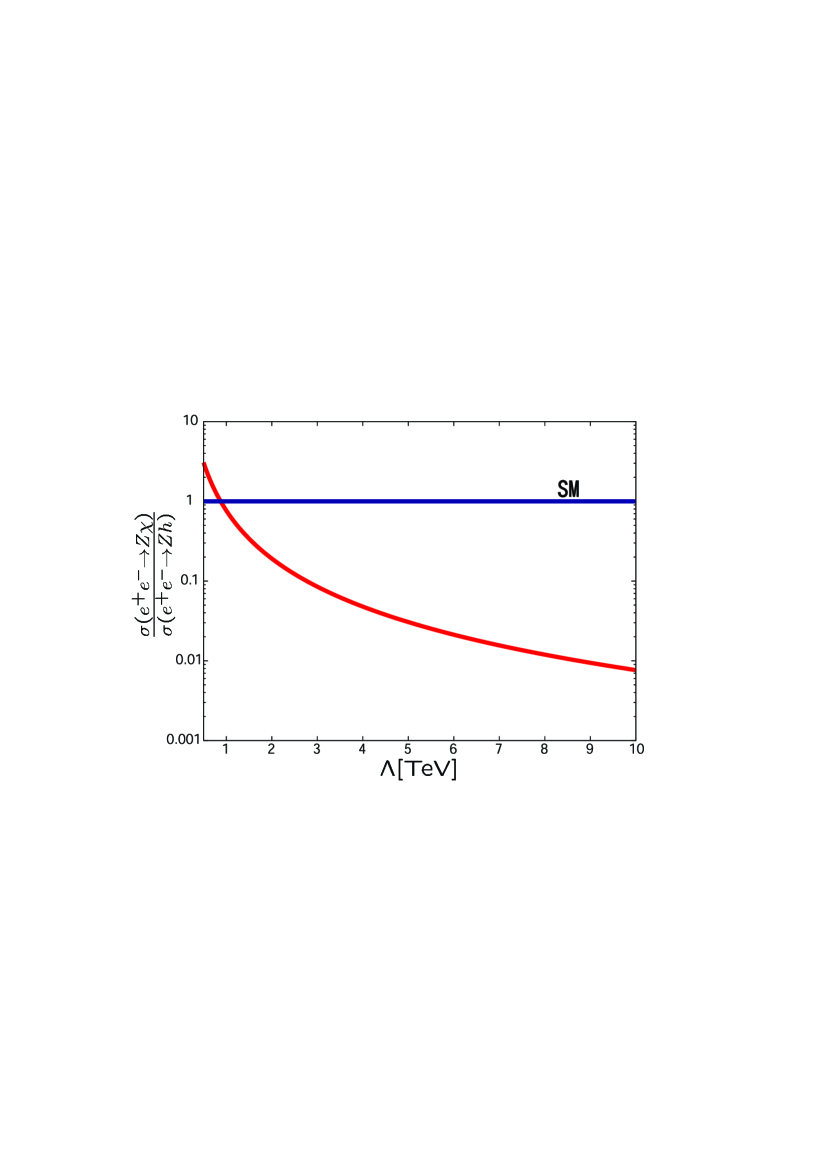
Figure 1: The ratio of total cross sections between the associated $\chi$ and Higgs productions as a function of $\Lambda$, at the ILC with the collider energy $\sqrt{s}=500$ GeV. Here, we have fixed the parameters such as $m_{\chi}=m_{h}=120$ GeV and $c_{1}=c_{2}=1$. The ratio becomes one for $\Lambda\simeq 872$ GeV.

where $\cos\theta$ is the scattering angle of the final state $Z$-boson, $g_{L}=2(m_{Z}/v)(-1/2+\sin^{2}\theta_{w})$, $g_{R}=2(m_{Z}/v)\sin^{2}\theta_{w}$, and $E_{Z}=\frac{\sqrt{s}}{2}\left(1+\frac{m_{Z}^{2}-m_{\chi}^{2}}{s}\right)$. It is interesting to compare this $\chi$ production process to the similar process of the associated Higgs production (Higgsstrahlung), $e^{+}e^{-}\rightarrow Zh$, through the Standard Model interaction ${\cal L}_{\rm int}=\frac{m_{Z}^{2}}{v}hZ^{\mu}Z_{\mu}$. In Figure 1, we show the ratio of the total cross sections between $\chi$ and Higgs boson productions as a function of $\Lambda$ at the ILC with the collider energy $\sqrt{s}=500$ GeV. Here we have taken $c_{1}=c_{2}$ and $m_{\chi}=m_{h}=120$ GeV. The ratio, $\sigma(e^{+}e^{-}\rightarrow Z\chi)/\sigma(e^{+}e^{-}\rightarrow Zh)$, becomes one for $\Lambda_{\rm IR}\simeq 872$ GeV, and it decreases proportionally to $1/\Lambda^{2}$. Note that in the high energy limit, the $\chi$ production cross section becomes energy-independent.

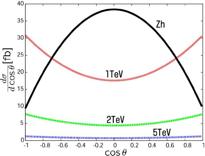
Figure 2: The angular dependence of the cross sections for $m_{\chi}=m_{h}=120$ GeV and $c_{1}=c_{2}=1$, at the ILC with the collider energy $\sqrt{s}=500$ GeV and $\Lambda=1$, $2$ and $5$ TeV.

The coupling manner among $\chi$ and the $Z$-boson pair is different from that of the Higgs boson. As can be understood from Eq. (3), $\chi$ couples with the transverse modes of the $Z$-bosons, while the Higgs boson mainly couples with the longitudinal modes. This fact reflects into the difference of the angular distribution of the final state $Z$-boson. In the high energy limit, we find $\frac{d\sigma}{d\cos\theta}(e^{+}e^{-}\rightarrow Z\chi)\propto 1+\cos^{2}\theta$, while $\frac{d\sigma}{d\cos\theta}(e^{+}e^{-}\rightarrow Zh)\propto 1-\cos^{2}\theta$. Figure 2 shows the angular distributions of the associated $\chi$ and Higgs boson productions, respectively. Even if $m_{\chi}=m_{h}$ and the cross sections of $\chi$ and Higgs boson productions are comparable, the angular dependence of the cross section can distinguish the $\chi$ production from the Higgs boson one.

The formula for the process $e^{+}e^{-}\rightarrow\gamma^{*},Z^{*}\rightarrow\gamma\chi$ can be easily obtained from Eq. (5) for $Z$-boson by the replacements: $c_{ZZ}\to c_{Z\gamma}$, $c_{Z\gamma}\to c_{\gamma\gamma}$ and $m_{Z}\rightarrow 0$. As a result, the cross section of the process $e^{+}e^{-}\rightarrow\gamma\chi$ is found to be

$$\frac{d\sigma}{d\cos\theta}(e^{+}e^{-}\rightarrow\gamma\chi)=\frac{1}{128\pi s}\sqrt{\frac{E_{\gamma}^{2}}{s}}\times$$

$$\left(c_{Z\gamma}^{2}(g_{L}^{2}+g_{R}^{2})\left(\frac{s}{s-m_{Z}^{2}}\right)^{2}-c_{Z\gamma}c_{\gamma\gamma}(g_{L}+g_{R})e\left(\frac{s}{s-m_{Z}^{2}}\right)+c_{\gamma\gamma}^{2}e^{2}\right)\frac{E_{\gamma}^{2}}{\Lambda_{\rm IR}^{2}}(1+\cos^{2}\theta),$$ (6)

where $E_{\gamma}=\frac{\sqrt{s}}{2}\left(1-\frac{m_{\chi}^{2}}{s}\right)$. For example, $\sigma(e^{+}e^{-}\rightarrow\gamma\chi)=105~{}{\rm fb}$ at $\sqrt{s}=500$ GeV with the parameter set: $m_{\chi}=120$ GeV, $c_{1}=c_{2}=1$ and $\Lambda=1$ TeV. For the Higgs production, the process $e^{+}e^{-}\rightarrow\gamma^{*}\rightarrow\gamma h$ is negligible.

Next, we consider $\chi$ decay processes into a pair of gauge bosons. Partial decay widths are given by

$$\Gamma(\chi\rightarrow gg) = \frac{c_{gg}^{2}}{8\pi}\frac{m_{\chi}^{3}}{\Lambda^{2}},$$

$$\Gamma(\chi\rightarrow\gamma\gamma) = \frac{c_{\gamma\gamma}^{2}}{64\pi}\frac{m_{\chi}^{3}}{\Lambda^{2}},$$

$$\Gamma(\chi\rightarrow ZZ) = \frac{c_{ZZ}^{2}}{512\pi}\frac{m_{\chi}^{3}}{\Lambda^{2}}\;\beta_{Z}\left(3+2\beta_{Z}^{2}+3\beta_{Z}^{4}\right),$$

$$\Gamma(\chi\rightarrow WW) = \frac{c_{WW}^{2}}{256\pi}\frac{m_{\chi}^{3}}{\Lambda^{2}}\;\beta_{W}\left(3+2\beta_{W}^{2}+3\beta_{W}^{4}\right),$$

$$\Gamma(\chi\rightarrow\gamma Z) = \frac{c_{Z\gamma}^{2}}{128\pi}\tan^{2}(2\theta_{w})\frac{m_{\chi}^{3}}{\Lambda^{2}}\;\left(1-\frac{m_{Z}^{2}}{m_{\chi}^{2}}\right)^{3},$$ (7)

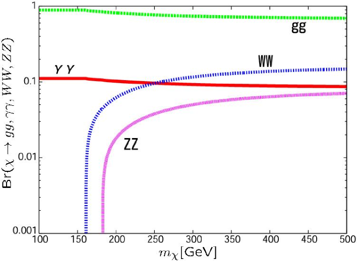
Figure 3: The branching ratio of the hidden scalar ($\chi$) as a function of its mass $m_{\chi}$ for $c_{1}=c_{2}=c_{3}=1$. Different lines correspond to the modes, $\chi\to gg$, $WW$, $\gamma\gamma$ and $ZZ$.

where $\beta_{Z}=\sqrt{1-4(m_{Z}/m_{\chi})^{2}}$, and $\beta_{W}=\sqrt{1-4(m_{W}/m_{\chi})^{2}}$. In Figure 3. the branching ratio of the $\chi$ decay is depicted. We see that the branching ratio of the $\chi$ decay is quite different from that of the Higgs boson. In particular, the branching ratio of $\chi\rightarrow\gamma\gamma$ can be large, ${\rm Br}(\chi\rightarrow\gamma\gamma)\simeq 0.1$ for the parameter set in Figure 3. On the other hand, the branching ratio of the Higgs boson into two photons in the SM is at most $10^{-3}$, since the coupling between the Higgs boson and two photons are induced through one-loop radiative corrections.

There are several models where the branching ratio of the Higgs boson into two photons is enhanced due to new physics effects. For example, in the MSSM with a large $\tan\beta$ [7], the lightest Higgs boson almost coincides with the up-type Higgs boson of the weak eigenstate. As a result, the Yukawa coupling to bottom quark is suppressed and two-photon branching ratio is relatively enhanced. Another example is the Next to MSSM (NMSSM), where a pseudo scalar ($A^{0}$) couples to the lightest (SM-like) Higgs boson. In this model, the Higgs boson can decay into two pseudo scalars ($h\rightarrow A^{0}A^{0}$) with a sizable branching ratio. If the pseudo scalar is extremely light (lighter than twice the pion mass), it dominantly decays into two photons ($A^{0}\rightarrow\gamma\gamma$), so that Higgs boson decays into four photons. Since the pseudo-scalar is very light, two photons produced in its decay are almost collinear and will be detected as a single photon [4]. As a result, the Higgs decay into two pseudo-scalars, followed by $A^{0}\rightarrow\gamma\gamma$, effectively enhances the Higgs branching ratio into two photons [4]. Therefore, the anomalous branching ratio alone is not enough to distinguish such a Higgs boson from $\chi$ (in the associated production with a $Z$-boson) and the measurements of angular distribution and polarization of the final state $Z$-boson are crucial.

Here, let us consider current experimental constraints on the parameters in our framework. Since the hidden scalar $\chi$ has the properties similar to the Higgs boson, we can use the current experimental limits of the Higgs boson search to constrain model parameters. The most severe constraint is provided by the Higgs boson search in the two-photon decay mode at Tevatron with the integrated luminosity 1 fb^-1, which is found to be $\sigma_{h}{\rm Br}(h\to\gamma\gamma)\lesssim 0.1$ pb for a light Higgs boson with a mass around 120 GeV [8]. Here, $\sigma_{h}$ is the Higgs boson production cross section at Tevatron, which is dominated by the gluon fusion process. The Standard Model predicts $\sigma_{h}{\rm Br}(h\to\gamma\gamma)\sim 10^{-3}$ pb, far below the bound. However, when this bound is applied to the $\chi$ production with $\Lambda\simeq 1$ TeV, we obtain a severe constraint on the model parameters. Comparing the couplings between gluons and $\chi$ to the one between gluons and the Higgs boson in the SM, we find the ratio of the production cross sections at Tevatron as $\sigma_{\chi}/\sigma_{h}\sim 100c_{gg}^{2}$. For $m_{\chi}=120$ GeV, for example, the main decay mode of the $\chi$ will be into two gluons and photons, and the branching ratio into two photons is estimated as ${\rm Br}(\chi\to\gamma\gamma)\simeq(c_{\gamma\gamma}/c_{gg})^{2}/9$. When we assume the universal coupling $c_{1}=c_{2}=c_{3}$ (equivalent to $c_{gg}=c_{\gamma\gamma}=c_{WW}=c_{ZZ}$ and $c_{Z\gamma}=0$), the Tevatron bound leads us to $c_{1}=c_{2}=c_{3}\lesssim 0.1$. However, in this case, the $\chi$ production cross section becomes two orders of magnitude smaller than the Higgs boson production cross section at the ILC.

There are many possible choices of the parameter set ($c_{1}$, $c_{2}$ and $c_{3}$) so as to satisfy the Tevatron bound, while keeping the $\chi$ production cross section to be comparable to the Higgs boson one. To simplify our discussion, in this paper, we choose a special parameter set: $c_{1}=c_{2}=1$ and $c_{3}=0$, namely the gluophobic but universal for $c_{1}$ and $c_{2}$. Therefore, the $\chi$ production channel through the gluon fusion is closed. For $m_{\chi}<2m_{W}$, the hidden scalar has a 100% branching ratio into two photons.

3 Monte Carlo Simulation

As estimated in the previous section, if the cutoff is around 1 TeV, the production cross section of the hidden scalar can be comparable to the Higgs boson production cross section at the ILC. There are two main production processes associated with a $Z$-boson or a photon. In the following, we investigate each process. In our analysis, we take the same mass for the hidden scalar and the Higgs boson: $m_{\chi}=m_{h}=120$ GeV, as a reference.

3.1 Observables to be measured

The associated hidden scalar production with a $Z$-boson is very similar to the Higgs production process and their production cross sections are comparable for $\Lambda\simeq 1$ TeV. One crucial difference is that the hidden scalar couples to $Z$-bosons through Eq. (3) so that the $Z$-boson in the final state is mostly transversely polarized. On the other hand, in the Higgs boson production the interaction between the Higgs boson and the longitudinal mode of the $Z$-boson dominates. In order to distinguish the hidden scalar from the Higgs boson, we will measure

(1) the angular distribution of the $Z$-boson in the final state,

(2) the polarization of the $Z$-boson in the final sate.

As shown in the previous section, the branching ratio of the hidden scalar decay is quite different from the Higgs boson one. In our reference parameter set, the hidden scalar decays 100% into two photons. The Higgs boson with $m_{h}=120$ GeV dominantly decays into a bottom and anti-bottom quark pair. In order to distinguish the hidden scalar from the Higgs boson, we will measure

(3) the branching ratios into two photons and into the bottom and anti-bottom quark pair through b-tagging.

The associated hidden scalar production with a photon is unique and such a process for the Higgs boson is negligible. We will investigate similar things as in the $Z$-boson case.

3.2 Analysis Framework

For Monte Carlo simulation studies of the hidden scalar productions and decays, we have developed event generators of the processes: $e^{+}e^{-}\to\gamma\chi$ and $e^{+}e^{-}\to Z\chi$ followed by the $\chi\to\gamma\gamma$ decay, which are now included in physsim-2007a [9]. In the helicity amplitude calculations, we retain the $Z$-boson wave function if any and replace it with the wave function composed with the daughter fermion-antifermion pair according to the HELAS algorithm [10]. This allows us to properly take into account the gauge boson polarization effects. The phase space integration and generation of parton 4-momenta are performed with BASES/SPRING [11]. Parton showering and hadronization are carried out using PYTHIA6.3 [12] with final-state tau leptons treated by TAUOLA [13] in order to handle their polarizations properly. The background $e^{+}e^{-}\to Zh$ events are generated using the $e^{+}e^{-}\to Z\chi$ generator with the $e^{+}e^{-}\to Z\chi$ helicity amplitudes replaced by corresponding $e^{+}e^{-}\to Zh$ amplitudes and the Higgs decay handled by PYTHIA6.3.

In the Monte Carlo simulations, we set the nominal center-of-mass energy at $500$ GeV and assume no beam polarization. Effects of natural beam-energy spread and beamstrahlung are taken into account according to the beam parameters given in [14]. We have assumed no crossing angle between the electron and the positron beams and ignored the transverse component of the initial state radiation. Consequently, the $Z\chi$ or $\gamma\chi$ system in our Monte-Carlo sample has no transverse momentum.

The generated Monte-Carlo events were passed to a detector simulator (JSF Quick Simulator [15]) which incorporates the ACFA-LC study parameters (see Table. 1). The quick simulator created vertex-detector hits, smeared charged-track parameters in the central tracker with parameter correlation properly taken into account, and simulated calorimeter signals as from individual segments, thereby allowing realistic simulation of cluster overlapping. It should also be noted that track-cluster matching was performed to achieve the best energy-flow measurements.

Detector	Performance	Coverage
Vertex detector	$\sigma_{\mathrm{b}}=7.0\oplus(20.0/p)\,/\,\sin^{3/2}\theta\;\mu\mathrm{m}$	$|\cos\theta|\leq 0.90$
Central drift chamber	$\sigma_{p_{T}}/p_{T}=1.1\times 10^{-4}p_{T}\>\oplus\>0.1\;\%$	$|\cos\theta|\leq 0.95$
EM calorimeter	$\sigma_{E}/E=15\;\%\>/\sqrt{E}\>\oplus 1\;\%$	$|\cos\theta|\leq 0.90$
Hadron calorimeter	$\sigma_{E}/E=40\;\%\>/\sqrt{E}\>\oplus 2\;\%$	$|\cos\theta|\leq 0.90$

Table 1: ACFA study parameters for an LC detector, where $p$, $p_{T}$, and $E$ are measured in units of GeV.

3.3 Event Selection and Results

3.3.1 $e^{+}e^{-}\to Z\chi;\chi\to\gamma\gamma$ process

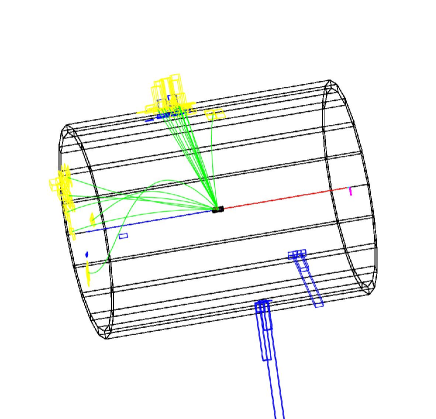
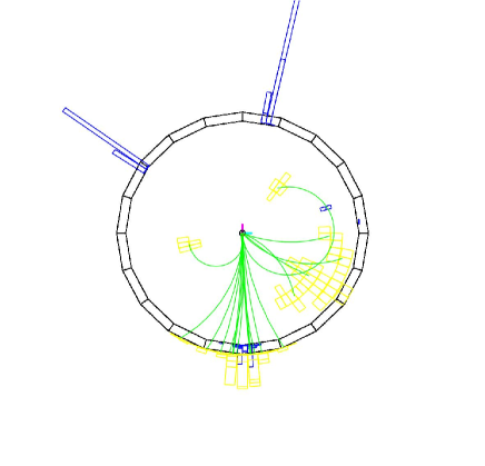
Figure 4: Event displays of $e^{+}e^{-}\to Z\chi$ followed by $\chi\to\gamma\gamma$. Two jets from the $Z$-boson decay and two photons from the $\chi$ decay can be clearly seen.

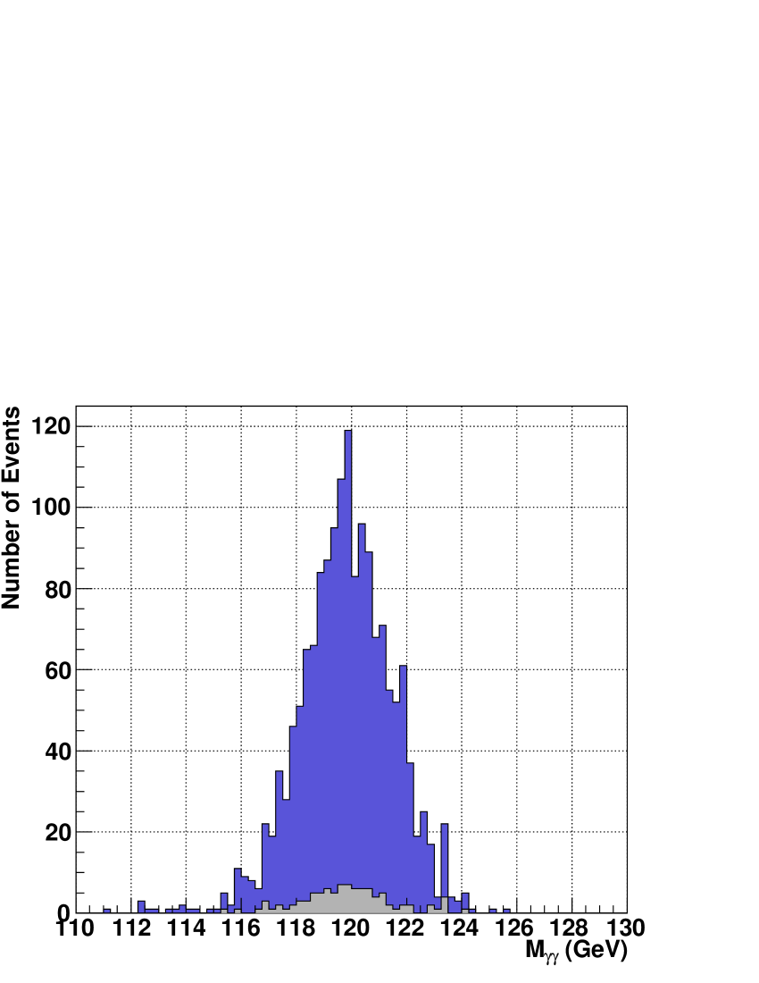
Figure 5: The distribution of the invariant mass of two photons which are considered to come from a $\chi$ decay.

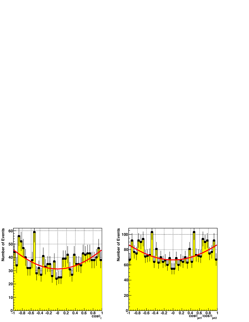
Figure 6: The $\chi$ production angle (left) and the angular distribution of the reconstructed jets from associated $Z$-boson decays (right).

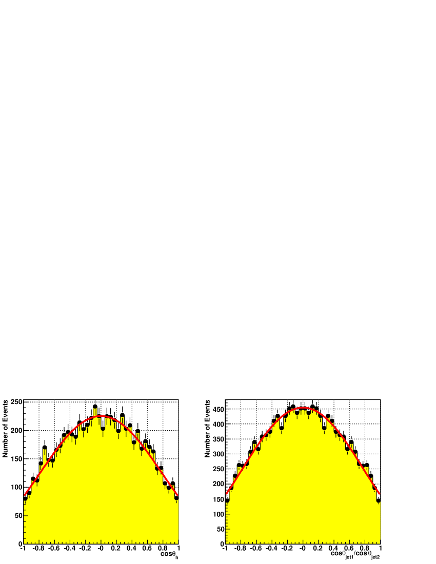
Figure 7: The Higgs production angle (left) and the angular distribution of the reconstructed jets from associated $Z$-boson decays (right) for $e^{+}e^{-}\to Zh$ followed by $H\to\gamma\gamma$.

Data equivalent to 50 fb^-1 have been generated for both $e^{+}e^{-}\to Z\chi$ followed by $\chi\to\gamma\gamma$ and $e^{+}e^{-}\to Zh$ followed by $h\to\gamma\gamma$. A typical event is displayed in Figure 4. For the $Z\chi\to q\bar{q}\gamma\gamma$ process, there are two jets and two photons in the final state. In the event selection, it is firstly required that the number of reconstructed particles ($N_{particles}$) is greater than 4. In the next, the number of photons reconstructed in the calorimeters ($N_{gammas}$) is greater than 2, and the two photons whose invariant mass is the closest to $m_{\chi}$ are selected. Finally, the number of jets ($N_{jets}$) is required to be equal to 2. These selection criteria are summarized in Table 2 together with efficiency of each cut. The distribution of the invariant mass of the two photons which are considered to come from a $\chi$ decay is shown in Figure 5 after imposing all the above selection criteria. In the figure, as a reference, we also plot the grey histogram corresponding to the $e^{+}e^{-}\to Zh$ process with the SM Higgs branching ratio where the number of remaining events is much less than that of the $e^{+}e^{-}\to Z\chi$ process. However, note that the large number of evens from the $\chi$ decay does not directly means that the $\chi$ has nothing to do with the electroweak symmetry breaking. As we discussed in the previous section, some class of new physics models can enhance the branching ratio of $h\to\gamma\gamma$ and so the number of events. If this is the case, the grey histogram becomes higher. Therefore, for the discrimination, it is crucial to measure the angular distribution and polarization of the final states. Figures 6 and 7 show the $\chi$ and Higgs production angles (left) and the angular distribution of the reconstructed jets from associated $Z$-boson decays (right) for the both processes, respectively. As can be seen from these plots, $\chi$ couples with the transverse modes of the $Z$-bosons, while the Higgs boson couples with the longitudinal modes. The $e^{+}e^{-}\to Zh$ followed by $h\to A^{0}A^{0}$ process is also analyzed with the same cut conditions and its cut statistics is summarized in Table 2. Here, we have assumed ${\rm Br}(h\to A^{0}A^{0})=0.1$ and ${\rm Br}(A^{0}\to\gamma\gamma)=1$. The distribution of the invariant mass of the two photons will be similar to Figure 5 in this model, but again we can discriminate the $\chi$ from the Higgs by looking at the angular distributions. Figure 8 shows the Higgs production angle and the angular distribution of the reconstructed jets from associated $Z$-boson decays (right) for the $h\to A^{0}A^{0}$ process.

Cut	$Z\chi;\chi\to\gamma\gamma$	$Zh;h\to\gamma\gamma$	$Zh;h\to A^{0}A^{0}$
No Cut	2187 (1.0000)	142 (1.000)	7087 (1.0000)
$N_{particles}\geq 4$	1738 (0.7947)	106 (0.747)	5692 (0.8032)
$N_{gammas}\geq 2$	1521 (0.8751)	96 (0.906)	4865 (0.8547)
Cut on $M_{\gamma\gamma}$	1499 (0.9855)	95 (0.990)	4828 (0.9924)
$N_{jets}=2$ for Ycut = 0.004	1498 (0.9993)	95 (1.000)	4825 (0.9994)
Total Efficiency	$0.6850\pm 0.0099$	$0.669\pm 0.040$	$0.6808\pm 0.0055$

Table 2: Cut statistics and breakdown of selection efficiency. The numbers inside and outside of parenthesis are the efficiency and the remaining number of events after each cut, respectively. Here, we have assumed ${\rm Br}(h\to A^{0}A^{0})=0.1$ and ${\rm Br}(A^{0}\to\gamma\gamma)=1$.

3.3.2 $e^{+}e^{-}\to\gamma\chi;\chi\to\gamma\gamma$ process

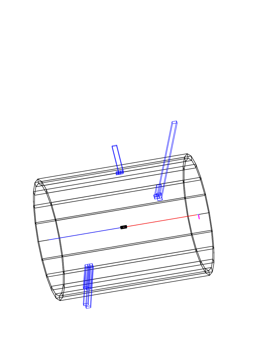
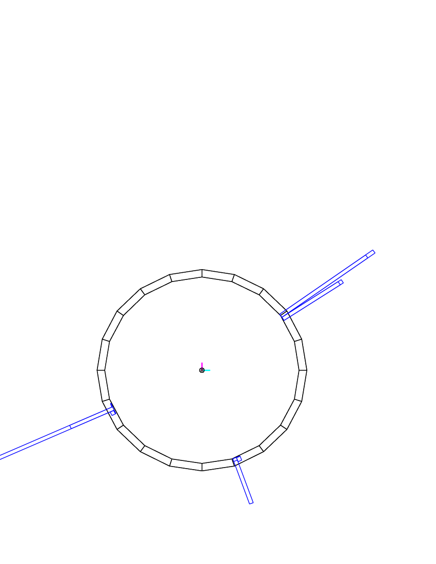
Figure 9: Event displays of $e^{+}e^{-}\to\gamma\chi$ followed by $\chi\to\gamma\gamma$.

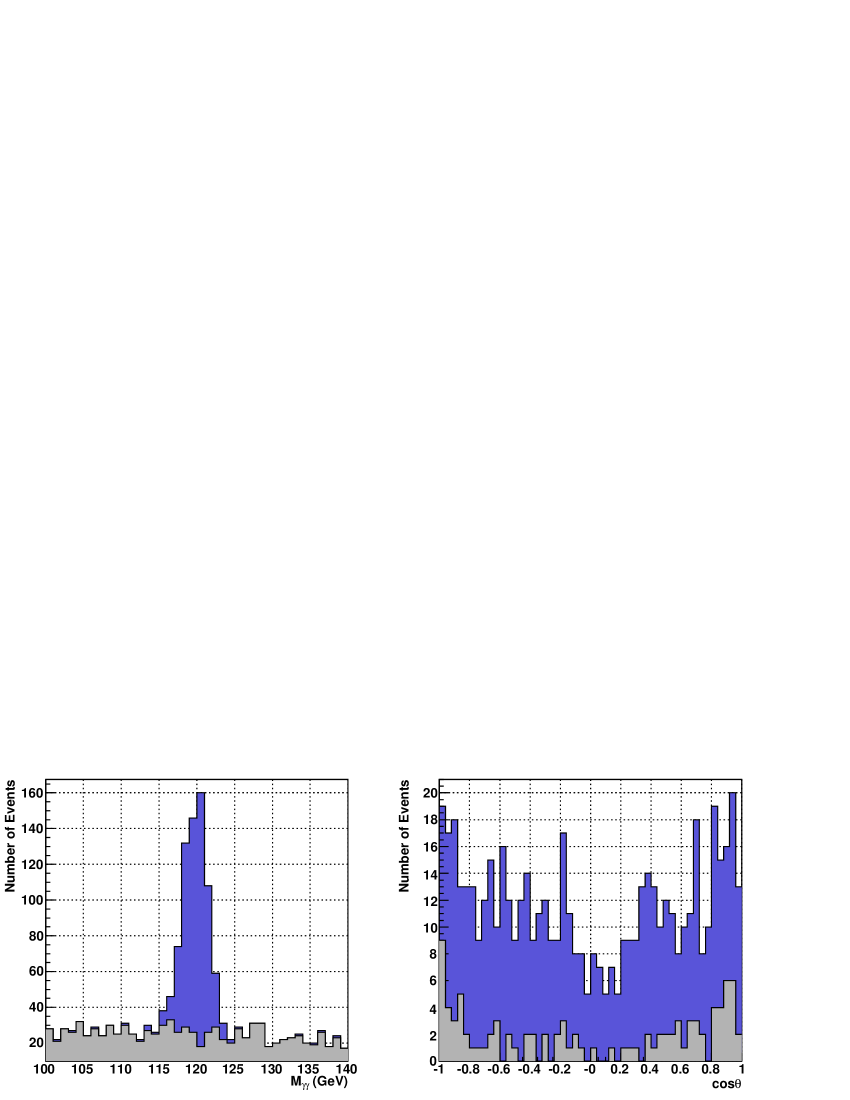
Figure 10: The distribution of the invariant mass of two photons which are considered to come from a $\chi$ decay (left) and the angular distribution of the $\chi$ (right) for the $e^{+}e^{-}\to\gamma\chi$ process with background.

Data equivalent to 5.7 fb^-1 have been generated for both signal ($e^{+}e^{-}\to\gamma\chi$ followed by $\chi\to\gamma\gamma$) and background ($e^{+}e^{-}\to\gamma\gamma$ with an ISR photon) processes. A typical signal event is displayed in Figure 9. For the $\gamma\chi\to\gamma\gamma\gamma$ process, there are three photons in the final state. The number of photons reconstructed in the calorimeters ($N_{gammas}$) is required to be equal to 3. It is also required that the energy and the cosine of the polar angle of each photon are greater than 1 GeV and less than 0.999, respectively. Among the photons, two photons whose invariant mass is within $m_{\chi}\pm 25$ GeV are considered to be from a $\chi$ decay. Finally, the cosines of the production angles of both $\chi$ and the remaining photon are required to be less than 0.99. These selection criteria are summarized in Table 3 together with their efficiencies. The distribution of the invariant mass of two photons which are considered to come from a $\chi$ decay (left) and the angular distribution of the $\chi$ (right) are shown in Figure 10 after imposing all the above selection criteria. A peak at $m_{\chi}$ can be clearly seen over the grey background histogram with the angular distribution consistent with $1+\cos^{2}\theta$.

Cut	$\gamma\chi;\chi\to\gamma\gamma$	$\gamma\gamma$ with an ISR
No Cut	600 (1.0000)	100000 (1.0000)
$N_{gammas}=3$	575 (0.9583)	3746 (0.0375)
$E_{gamma}>1$ GeV	575 (1.0000)	3730 (0.9959)
$|\cos(\theta_{j})|\leq 0.999$	575 (1.0000)	3728 (0.9992)
$|M_{\gamma\gamma}-m_{\chi}|\leq 25$ GeV	573 (0.9965)	1332 (0.3573)
$|\cos(\theta_{\chi})|$ and $|\cos(\theta_{a})|\leq 0.99$	572 (0.9983)	1269 (0.9529)
Total Efficiency	$0.9533\pm 0.0086$	$0.0127\pm 0.0001$

Table 3: Similar to Table 2 for $e^{+}e^{-}\to\gamma\chi$ and $e^{+}e^{-}\to\gamma\gamma$ with an ISR photon.

4 Summary and discussions

If a hidden scalar field appears in a certain class of new physics models around the TeV scale, there are interesting implications for collider phenomenology. In particular, since the scalar behaves like the Higgs boson in its production process, it is an interesting issue how to distinguish the scalar from the Higgs boson in future collider experiments. We investigated the hidden scalar production at the ILC and addressed this issue based on realistic Monte Carlo simulations.

With the $\chi$ production cross section comparable to the Higgs boson one, the invariant mass distribution reconstructed from two-photon final states due to the decay mode $\chi\to\gamma\gamma$ shows a clear peak at $m_{\chi}$. In the $\chi$ production associated with a $Z$-boson, the $\chi$ production angle and the angular distribution of the reconstructed jets from the associated $Z$-boson decay reveal that the hidden scalar couples to transversally polarized $Z$-bosons. On the other hand, the Higgs boson production associated with a $Z$-boson shows clearly different results in angular distributions and distinguishable from the hidden scalar production.

Some comments are in order here. In this paper, we have assumed that the hidden scalar couples with only the SM gauge bosons. In general, one can introduce couplings between the hidden scalar and the SM fermions and the Higgs doublets. Once these couplings are introduced, the phenomenology of $\chi$ productions can be drastically altered from those in this paper. In particular, the coupling of the hidden scalar to the Higgs doublets induces the mixing between $\chi$ and the Higgs boson. This mixing spoils the crucial difference between the hidden scalar and the Higgs boson that the former has nothing to do with the electroweak symmetry breaking while the latter is crucial for it. It is not natural but in practice, we can assume the above unwanted couplings to be small.

In fact, it is easy to introduce a setup where the couplings are naturally suppressed. As a simple example, let us consider a model in the context of the brane world scenario, where there are two different branes with the three spatial dimensions separated in extra-dimensional directions. Suppose that the SM gauge bosons live in the bulk and the hidden scalar resides on one brane while the SM fermions and the Higgs doublets on the other brane. In this setup, the couplings between the hidden scalar and the SM fermions and Higgs doublets are geometrically suppressed, while the hidden scalar couples with the bulk SM gauge bosons. However, considering loop corrections through gauge bosons, the mixing term between Higgs doublet ($H$) and $\chi$ can be induced which is roughly estimated as

$${\cal L}_{int}\sim\frac{\alpha_{2}}{4\pi}\Lambda\chi(H^{\dagger}H),$$ (8)

where $\alpha_{2}$ is the SM SU(2) gauge coupling and we have cut off the quadratic divergence of this loop calculation by $\Lambda$. After the Higgs doublet develops the VEV, a mass mixing between $\chi$ and the Higgs boson arises. Mixing angle is roughly estimated as $\frac{\alpha_{2}}{4\pi}\Lambda v/m_{\chi}^{2}\sim 0.05$ for the Higgs VEV $v=246$ GeV, $\Lambda\simeq 1$ TeV and $m_{\chi}=120$ GeV. Thus, only the 5% of the Higgs boson couples to the transverse mode of the $Z$-boson (only the 5% of $\chi$ couples to the longitudinal mode of the $Z$-boson), and there is no great importance for our purpose of this paper, though it would be rather interesting how accurately the ILC can measure this mixing. While the modification of the $\chi$ decay due to the 5% mixing (at least, for the parameters we chose) is negligible, this mixing can greatly enhance the Higgs branching into two photons as in the models with $A_{0}$.

In our analysis, we have taken a special parameter set for simplicity, namely, the gluophobic ($c_{3}=0$) and universal ($c_{2}=c_{1}$) couplings considering the Tevatron bound. In general, it is not necessary to take $c_{3}=0$ in order to avoid the Tevatron bound. For example, a parameter set, $c_{gg}=c_{\gamma\gamma}=0.1$ and $c_{ZZ}=1$, can be consistent with the Tevatron bound while keeping the $\chi$ production cross section comparable to that of Higgs boson. In this case, $c_{Z\gamma}\simeq 0.7$ and the hidden scalar decays into $Z\gamma$ with a sizable branching ratio. It is interesting to study the $\chi$ production through its decay into $Z\gamma$. Also, in this parameter set, the decay mode into two gluons is sizable. It is hence an interesting issue how to distinguish $\chi$ from the Higgs boson through their hadronic decay modes. As can be seen from Eq. (5), the coupling between the hidden scalar and the longitudinal mode of the $Z$-boson is proportional to $m_{Z}/E_{Z}$ and is sizable at low energy. To measure this coupling through the energy-dependence of the production angle distribution may provide an additional handle to pin down the $\chi$ production. For this purpose, the ILC with low energy could be useful.

In this paper, we have concentrated on the hidden scalar production associated with a $Z$-boson or a photon. It is also interesting to investigate the weak boson fusion process. For example, in the $Z$-boson fusion process, measuring the correlations between the cross section and the azimuthal angle between the final state electron and positron can be used to distinguish the couplings between a scalar and the $Z$-boson with different polarizations.

Acknowledgments

This work is supported in part by the Creative Scientific Research Grant (No. 18GS0202) of the Japan Society for Promotion of Science (K.F., H.H., H.I. and T.Y.) and the Grant-in-Aid for Scientific Research from the Ministry of Education, Science and Culture of Japan, No. 18740170 (N.O.).

Figure 8: The Higgs production angle (left) and the angular distribution of the reconstructed jets from associated $Z$-boson decays (right) for $e^{+}e^{-}\to Zh$ followed by $h\to A^{0}A^{0}$.

References

- [1] N. Arkani-Hamed, S. Dimopoulos and G. Dvali, Phys. Lett. B429, 263 (1998); I. Antoniadis, N. Arkani-Hamed, S. Dimopoulos and G. Dvali, Phys. Lett. B436, 257 (1998); N. Arkani-Hamed, S. Dimopoulos and G. Dvali, Phys. Rev. D59, 086004 (1999).
- [2] L. Randall and R. Sundrum, Phys. Rev. Lett. 83, 3370 (1999).
- [3] See, for example, J. F. Gunion, H. E. Haber, G. L. Kane and S. Dawson, The Higgs Hunter’s Guide, Addison-Weseley: Redwood City, California, 1989.
- [4] B. A. Dobrescu, G. L. Landsberg and K. T. Matchev, Phys. Rev. D 63, 075003 (2001).
- [5] H. Itoh, N. Okada and T. Yamashita, Phys. Rev. D 74, 055005 (2006).
- [6] H. Georgi, Phys. Rev. Lett. 98, 221601 (2007).
- [7] H. Baer and J. D. Wells, Phys. Rev. D 57, 4446 (1998) [arXiv:hep-ph/9710368]; W. Loinaz and J. D. Wells, Phys. Lett. B 445, 178 (1998) [arXiv:hep-ph/9808287]; M. S. Carena, S. Mrenna and C. E. M. Wagner, Phys. Rev. D 60, 075010 (1999) [arXiv:hep-ph/9808312]; Phys. Rev. D 62, 055008 (2000) [arXiv:hep-ph/9907422].
- [8] S. Mrenna and J. D. Wells, Phys. Rev. D 63, 015006 (2000) [arXiv:hep-ph/0001226].
- [9] physsim-2007a, http://www-jlc.kek.jp/subg/offl/physsim/ .
- [10] H. Murayama, I. Watanabe and K. Hagiwara, KEK Report, 91-11 (1992).
- [11] S. Kawabata, Comp. Phys. Commun. 41, 127 (1986).
- [12] T. Sjöstrand, L. Lönnblad, S. Mrenna, P. Skands, hep-ph/0308153 (2003).
- [13] S. Jadach, Z. Was, R. Decker and J. H. Kühn, Comp. Phys. Commun. 76, 361 (1993).
- [14] GLD Detector Outline Document.
- [15] JSF Quick Simulator, http://www-jlc.kek.jp/subg/offl/jsf/ .