Doped AB₂ Hubbard Chain: Spiral, Nagaoka and RVB States, Phase Separation and Luttinger Liquid Behavior

Abstract

We present an extensive numerical study of the Hubbard model on the doped AB₂ chain, both in the weak coupling and the infinite-U limit. Due to the special unit cell topology, this system displays a rich variety of phases as function of hole doping ($\delta$) away from half-filling. Near half-filling, spiral states develop in the weak coupling regime, while Nagaoka itinerant ferromagnetism is observed in the infinite-U limit. For higher doping the system phase-separates before reaching a Mott insulating phase of short-range RVB states at $\delta=1/3$. Moreover, for $\delta>1/3$ we observe a crossover, which anticipates the Luttinger liquid behavior for $\delta>2/3$.

I Introduction

Low-dimensional strongly correlated electron systems have attracted great attention in the last two decades. The reason dates back to Anderson’s proposal anderson_sce that the $t-J$ version of the Hubbard model might carry the basic mechanisms underlying the high-Tc superconductivity observed in CuO₂ compounds. Despite that this remains an open issue, the above suggestion fertilized intensive investigations on many related fundamental topics, such us itinerant electron magnetism, Mott metal-insulator transitions and quantum critical phenomena. Amongst several features of interest, we mention the possibility of realization of spiral spiral , Nagaoka nagaoka ; tasaki ; yso and resonating-valence-bond (RVB) states rvb , spatially separated phases emery ; dagotto and Luttinger liquid behavior luttinger , which may present strong deviations from the Landau Fermi liquid theory.

In this work, we report numerical results of the Hubbard model on the doped AB₂ chain away from half filling, which show that its special unit cell topology greatly enriches the phase diagram found in the doped standard linear chain. In fact, all features mentioned above are shown to be associated with well defined ground state (GS) phases of this doped chain. Doped AB₂-Hubbard chains were previously studied through Hartree-Fock, quantum monte carlo and exact diagonalization (ED) techniques both in the weak and strong coupling limits PRLMDCF , including also the $t-J$ model white using density matrix renormalization group (DMRG) and recurrent variational Ansätzes, and the infinite-U limit JPSPW using ED. In particular, these chains represent an alternative route to reaching two-dimensional quantum physics from one-dimensional systems Delgado ; white . At half filling the AB₂-Hubbard chain exhibits a quantum ferrimagnetic GS PRBTIAN ; CELSO ; PRLMDCF ; PHYSARRMF , whose magnetic excitations have been studied in detail both in the weak and strong coupling limits PHYSARRMF , and in the light of the quantum Heisenberg model PHYSARRMF ; SW . Further studies have considered the anisotropic CINV and isotropic NLS critical behavior of the AB₂-quantum-Heisenberg model, including its spherical version QSM , and the statistical mechanics of the AB₂-classical-Heisenberg model JPHYSA .

On the experimental side, the AB₂ chain topology is of relevance to the understanding of the physics of some low-dimensional strongly correlated electronic systems. One class is the line of trimer clusters present in fosfates with formula A₃Cu₃(PO₄)₄, where A=Ca JBAnderson ; Drillon ; Belik ; Matsuda , Sr Boukhari ; Drillon ; Belik ; Matsuda and Pb Eff ; Belik ; Matsuda . The trimers have three Cu²⁺ ($S=1/2$) paramagnetic ions antiferromagnetically coupled. Although the superexchange intertrimer interaction is much weaker than the intratrimer coupling, it proves sufficient to turn them bulk ferrimagnets. Another quasi-one-dimensional inorganic material closely associated with the ferrimagnetic phase of the AB₂ chain is the NiCu bimetallic chain NICU . These compounds display alternating Ni²⁺ ($S=1$) and Cu²⁺ ($S=1/2$) ions connected through suitable ligands in a line; and are modeled by the alternating spin-$\frac{1}{2}$/spin-1 antiferromagnetic Heisenberg chain spin1_2spin1 . We also would like to mention a more recently synthesized organic ferrimagnetic compound consisting of three $S=1/2$ paramagnetic radicals ORG in its magnetic unit cell, as well as possible connections with the physics of the oxocuprates oxoc .

This paper is organized as follows: in Sec. II we introduce the model system and the numerical techniques used to calculate several quantities suitable to characterize the occurrence of distinct phases as function of doping and Coulomb coupling. In Sec. III, we discuss spiral and Nagaoka states at low hole doping, whose magnetic properties are shown to exhibit very interesting features in the weak and infinite-U limit, respectively. In Sec. IV we show that for higher hole doping the system phase separates, before reaching a Mott insulating phase of short-range RVB states at $\delta=1/3$. In Sec. V we discuss several features of the crossover region, which takes place before the Luttinger liquid behavior observed for $\delta>2/3$. Finally, in Sec. VI we present a summary and some conclusions concerning the reported results.

II Model description and Methods

The AB₂ chain is a bipartite lattice with three sites (named A, B₁ and B₂) per unit cell, as illustrated in Fig. 1(a). The Hubbard Hamiltonian for a lattice with $N_{c}$ unit cells and $N$ sites reads:

$$H=-t\sqrt{2}\sum_{l=1,\sigma}^{N_{c}}[b_{l\sigma}^{\dagger}(A_{l\sigma}+A_{l+1,\sigma})+\mbox{H.c.}]+U\sum_{i=1}^{N}n_{i\uparrow}n_{i\downarrow},$$ (1)

where $A_{l\sigma}^{\dagger}$ and $b_{l\sigma}^{\dagger}=\frac{1}{\sqrt{2}}(B_{1,l\sigma}^{\dagger}+B_{2,l\sigma}^{\dagger})$ are the creation operators of an electron with spin $\sigma$ at site A and in a bonding state between sites $B_{1}$ and $B_{2}$ of the cell $l$, respectively, $t(\equiv 1)$ is the hopping amplitude and $U$ is the Coulomb coupling. For $U=\infty$, double occupancy is completely excluded and the Hamiltonian takes the form:

$$H=-t\sqrt{2}\sum_{l=1,\sigma}^{N_{c}}P_{G}[b_{l\sigma}^{\dagger}(A_{l\sigma}+A_{l+1,\sigma})+\mbox{H.c.}]P_{G},$$ (2)

where $P_{G}=\prod_{i}(1-n_{i\uparrow}n_{i\downarrow})$ is the Gutzwiller projector operator. The model is invariant under the interchange of the $B$ sites of the same cell, a symmetry that implies in a well defined local parity ($p_{l}=\pm 1$) for the GS wave function. As a result, in computing some quantities we find it convenient to use the effective linear chain (ELC) generated by the map illustrated in Figs. 1(a) and 1(b), i. e., any quantity $X_{B,l}$ associated with a $B$ site at cell $l$ of the ELC is given by $X_{B_{1},l}+X_{B_{2},l}$. This mapping does not change the physical content of the GS and excited states, being used only to expose in a more clear fashion some properties of these states.

In the tight-binding description ($U=0$) this model presents three bands PRLMDCF : one flat with $N_{c}$ odd parity states [antibonding orbitals, $a^{\dagger}_{l\sigma}=\frac{1}{\sqrt{2}}(B^{\dagger}_{1,l\sigma}-B^{\dagger}_{2,l\sigma}$)] and energy $\epsilon=0$; and two dispersive branches,

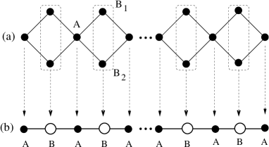
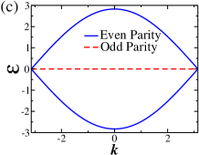
Figure 1: (Color online). (a) Illustration of the $AB_{2}$ chain showing $A$, $B_{1}$ and $B_{2}$ sites; (b) Illustration of the effective linear chain (ELC). (c) Electronic bands of the tight-binding model: two dispersive (continuous line) and one flat (dashed line).

$$\epsilon_{\pm}(k)=\pm 2\sqrt{2}\cos(k/2),$$ (3)

with $k=2\pi l/N_{c}$, $l=0,1,2,...,N_{c}-1$, built from A sites and bonding (even parity) orbitals, as shown in Fig. 1(c). At half filling ($N_{e}=N$, where $N_{e}$ is the number of electrons) the GS total spin $S_{g}$ is degenerate, with $S_{g}$ ranging from the minimum value ($0$ or $1/2$) to $S_{g}=|N_{B}-N_{A}|/2$, where $N_{A}(N_{B})$ is the number of sites in the A (B) sublattice. As proved by Lieb PRLLIEB the Coulomb repulsion lifts this huge degeneracy and selects the

$$S_{g}=|N_{B}-N_{A}|/2\equiv S_{Lieb}$$ (4)

ground state for any finite $U$, giving rise to a ferrimagnetic GS PRBTIAN ; PRLMDCF ; PHYSARRMF .

On the other hand, for $U=\infty$, one hole ($N_{e}=N-1$) and periodic boundary conditions (BC’s), the system satisfies the requirements of Nagaoka’s theorem for saturated ferromagnetism PRLMDCF ; JPSPW . For Nagaoka ferromagnetism and Lieb ferrimagnetism the GS is homogeneous in parity with $p_{l}=-1$ for any cell $l$. Due to this symmetry, the spectrum of the AB₂ chain in the Heisenberg limit ($U>>t$, $N_{e}=N$) at the sector $p=-1$ is identical to that of the alternating Heisenberg spin-$\frac{1}{2}$/spin-1 chain spin1_2spin1 .

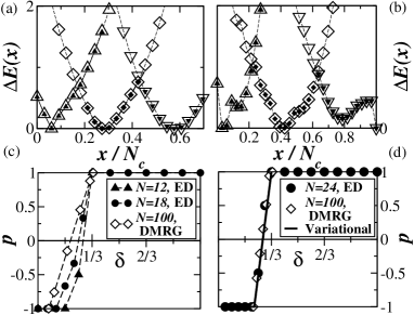
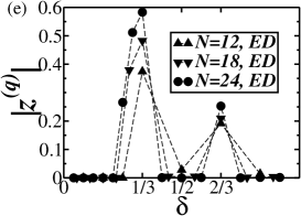
Figure 2: DMRG results for the energy difference between the lowest energy at the symmetry sector $(-)^{x}(+)^{N_{c}-x}$ and the GS energy for $N=100$ ($N_{c}=33$) for (a) $U=2$ at $\delta=0.32$ (triangle up), $\delta=0.26$ (diamond) and $\delta=0.18$ (triangle down); (b) $U=\infty$ at $\delta=0.32$ (triangle up), $\delta=0.28$ (triangle up) and $\delta=0.24$ (triangle down), taking 108 states per block (open symbols) and 216 states per block (filled symbols). Average local parity $p$ as function of $\delta$ for (c) $U=2$ and (d) $U=\infty$. (e) ED results for $|z^{(q)}|$. Dashed lines are guides to the eye.

Here we focus on the effect of hole doping, $\delta=1-(N_{e}/N)$, both in the weak coupling and the infinite-U limit, using exact diagonalization (ED) through the Lanczos algorithm for closed BC’s and DMRG for open BC’s dmrg1 . In the ED procedure, the BC’s are such to minimize the energy, except for $U=2$ and $\delta\leq 1/3$ [Fig. 2(c)] in which the BC’s (periodic or antiperiodic) are such that the Fermi wave vector $k_{F}$ in the thermodynamic limit is included in the set of wave vectors for the finite system julien . We used finite size DMRG for open chains with A sites in its extrema, keeping 364 to 546 states per block in the last sweep. The maximum discarded weight in the last sweep was typically $\thicksim 10^{-7}$, except for odd phases and $U=2$, where the discarded weight was $\thicksim 10^{-5}$. In the DMRG calculations we treated $B_{1}$ and $B_{2}$ as a composite site with 9 states for $U=\infty$ and 16 states for $U=2$. However, by considering the parity symmetry, we can decompose this supersite into the two possible symmetry sectors $+1$ and $-1$ . Within this scheme, we have considered all parity symmetry sectors of the form $(-)^{x}(+)^{N_{c}-x}$, with $x$ contiguous cells of odd parity in one side of the open chain and $N_{c}-x$ contiguous cells of even parity in the other. In addition, we have verified the stability of this phase separation against the formation of a mixed phase composed of smaller domains. The energy is studied as function of $x$ for increasing number of states kept per block in order to localize the value of $x$ for which the energy is minimum, as shown in Figs. 2(a) and 2(b). The phase-separated boundaries are thus determined by the limiting dopings for which an inhomogeneous phase (non-uniform parities) is observed. We have also developed a simple variational approach for $U=\infty$ and $\delta\leq 1/3$, which is explained in detail in Appendix A. The results calculated using this approach are shown in Figs. 2(d) and 3(c).

In Fig. 2(c) ($U=2$) and Fig. 2(d) ($U=\infty$) we present the average parity,

$$p\equiv\frac{1}{N_{c}}\sum_{l=1}^{N_{c}}p_{l},$$ (5)

as function of doping, computed using the above-mentioned methods. In both regimes, we observe the occurrence of an homogeneous phase near half filling with $p=-1$. For higher doping, i. e., $\delta_{\mbox{PS}}(U)<\delta<(1/3)$ [$\delta_{\mbox{PS}}(2)\approx 0.07$ and $\delta_{\mbox{PS}}(\infty)\approx 0.22]$ the system phase separates in one region with odd parity cells and the other with even ones. For $\delta\geq 1/3$ the GS is homogeneous with $p=1$.

In order to present an overview of the conducting properties of the $AB_{2}$ chain phases in the infinite-U limit, we display in Fig. 2(e) the quantity zq

$$|z^{(q)}|=|\langle\exp{(\frac{2\pi qi}{L}\sum_{j}{x_{j}})}\rangle|,$$ (6)

calculated in the ELC using ED, where $L=2N_{c}$, $x_{j}=jn_{j}$, $n_{j}$ is the electron density at site $j$ and $q$ is such that $\frac{N_{e}}{L}=\frac{p}{q}$, with $p$ and $q$ co-primes. The phase of $z^{(q)}$ corresponds to the GS expectation value of the position operator, while its modulus defines the localization length; in an insulator, $|z^{(q)}|\rightarrow 1$, as $L\rightarrow\infty$, while in a conductor, $|z^{(q)}|\rightarrow 0$, for closed boundary conditions zq . The increase of $|z^{(q)}|$ with system size for $\delta=2/3\mbox{ and }1/3$, as well as in the phase separated region, are evidences of insulating phases at these dopings. These conclusions will be better fundamented by studying the Drude weight using ED and the charge gap for larger systems with DMRG.

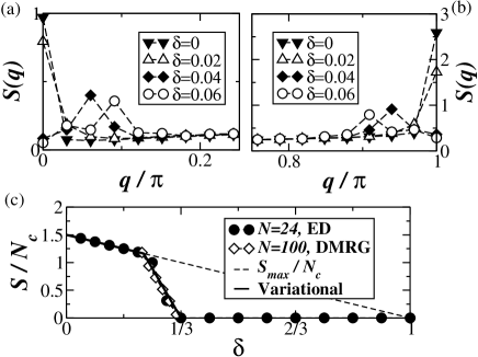
Figure 3: (a) and (b): Magnetic structure factor for $U=2$ and $N=100$ in the underdoped region. (c) Total spin per cell $S/N_{c}$ as function of $\delta$ for $U=\infty$.

III Spiral states and Saturated ferromagnetism

In Figs. 3(a) and 3(b) we display the magnetic structure factor

$$S(q)=\frac{1}{S_{Lieb}(S_{Lieb}+1)}\sum_{l,m}^{2Nc+1}e^{iq(l-m)}\langle\mathbf{S}_{l}\cdot\mathbf{S}_{m}\rangle,$$ (7)

calculated at $S^{z}=0$ and $U=2$ using DMRG for the ELC. First, notice the presence of peaks at $q=0$ and $q=\pi$ revealing the ferrimagnetic order at half filling. These peaks sustain up to two holes ($\delta=0.02$); however, it is not clear whether the ferrimagnetic phase is robust against doping in the thermodynamic limit. Indeed, by increasing the hole doping, spiral peaks at $\delta$-dependent positions appear near $q=0$ and $q=\pi$. The analysis of the charge gap,

$$\Delta_{c}=E(N_{e}+1)+E(N_{e}-1)-2E(N_{e}),$$ (8)

suggests that these states are metallic, in opposition to the Mott insulating ferrimagnetic state at $\delta=0$. It is worth mentioning that the occurrence of spiral phases in oxocuprates has been a challenging and topical subject oxoc .

In Fig. 3(c) we present the GS total spin as function of doping for $U=\infty$. For $\delta<\delta_{\mbox{PS}}(\infty)$ itinerant saturated ferromagnetism due to hole kinematics (Nagaoka mechanism) is observed. It is interesting to notice that our estimate for the upper hole density ($\gtrsim 0.2$) beyond which Nagaoka ferromagnetism is unstable is in very good agreement with similar predictions for ladders troyer ; 1D_F and the square lattice 2D_F .

We have also considered the presence of an Aharonov-Bohn flux $\Phi$ for a closed chain through the gauge transformation:

$$\left\{\begin{array}[]{ccc}b_{l\sigma}&\rightarrow&b_{l\sigma}\mbox{e}^{2\pi\Phi l/N_{c}};\\ A_{l\sigma}&\rightarrow&A_{l\sigma}\mbox{e}^{2\pi\Phi l/N_{c}},\end{array}\right.$$ (9)

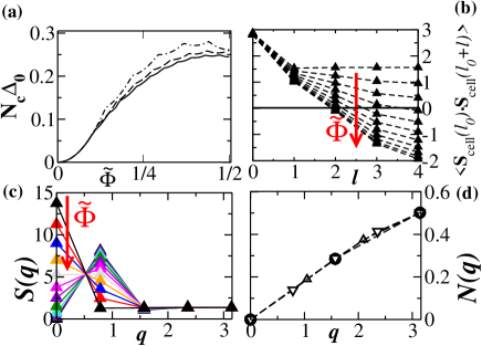
Figure 4: (Color online). ED results of (a) $N_{c}$ times the energy gap $\Delta_{0}$ between the saturated ferromagnetism energy ($\Phi=\Phi_{F}$) and the lowest energy state for an Aharanov Bohn flux $\Phi$ as function of $\widetilde{\Phi}=|\Phi-\Phi_{F}|$ at $\delta=1/6$ and $N_{c}=$ 4 (dashed-dot line), 6 (dashed line) and 8 (solid line). ED calculation for the $\widetilde{\Phi}$ dependent behavior of the (b) Spin correlation function $\langle\mathbf{S}_{\mbox{cell}}(l_{0})\cdot\mathbf{S}_{\mbox{cell}}(l_{0}+l)\rangle$ between the cell spins as function of $l$ and (c) magnetic structure factor as function of lattice wave vector $q$ at $\delta=1/6$. (d) Charge structure factor calculated at the lowest energy state for any $\widetilde{\Phi}$ at $\delta=1/6$ for $N_{c}=$ 4 ($\bullet$), 6 ($\blacktriangle$) and 8 ($\triangledown$).

with $\Phi_{0}=hc/e\equiv 1$. The flux variation is equivalent to a change in the boundary condition: $\Phi=0$ represents periodic and $\Phi=1/2$ antiperiodic boundary conditions. In Fig. 4(a) we present the dependence of the energy gap $\Delta_{0}$ between the lowest energy state for a flux $\Phi$ and that for saturated ferromagnetism ($\Phi\equiv\Phi_{F}$) as function of $\widetilde{\Phi}=|\Phi-\Phi_{F}|$ at $\delta=1/6$. We have identified many level crossings in this curve. In fact, as the flux increases from $\Phi_{F}$, the total spin decreases from the maximum value, $S=N_{e}/2$, to the minimum value $S=0$ ($S=1/2$) for $N_{e}$ even (odd), a behavior also observed in the square lattice kusakabe . Notice that $N_{c}\Delta_{0}$ tends to saturation with system size, indicating that the level spacings decrease with $1/N_{c}$. These results suggest that the thermodynamic GS displays spontaneously SU(2) symmetry breaking as a result of an ergodic combination of infinitely many states ($N_{c}\rightarrow\infty$), including the singlet spiral state koma_e_tasaki . In Figs. 4(b) and 4(c) we present the spin correlation function between cell spins $\mathbf{S}_{cell}(l)=\mathbf{S}_{A}(l)+\mathbf{S}_{B_{1}}(l)+\mathbf{S}_{B_{2}}(l)$ and the magnetic structure factor

$$S(q)=\frac{1}{N_{c}}\sum_{\langle l,m\rangle}e^{iq(l-m)}\langle\mathbf{S}_{cell}(l)\cdot\mathbf{S}_{cell}(m)\rangle$$ (10)

as function of distance $l$ and wave vector $q=2\pi l/N_{c}$, $l=0,...,N_{c}$, respectively. As we can observe, the saturated ferromagnetic and the spiral singlet states are adiabatically connected, such that all states contributing to the thermodynamic GS exhibit long-range ordering. In particular, as the flux increases from $\Phi_{F}$ the peak of $S(q)$ at $q=0$ (saturated ferromagnetism) steadily decreases, while the spiral state peak at $q=2\pi/N_{c}$ increases. We noted also that the charge structure factor

$$N(q)=\frac{1}{N_{c}}\sum_{\langle l,m\rangle}e^{iq(l-m)}\langle\Delta n_{l}\Delta n_{m}\rangle,$$ (11)

where $\Delta n_{l}=n_{l}-\langle n_{l}\rangle$ and $n_{l}$ is the electron occupation number at cell $l$, is not affected by the flux variation and displays a peak at $2k_{F}=\pi$ [Fig. 4(d)], where $k_{F}$ is the tight-binding spinless Fermi wave vector PRLMDCF , with $k_{F}=3\pi\delta$, $\delta\leq 1/3$.

IV Phase separation and RVB states

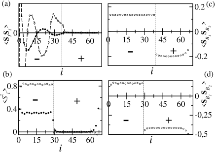
Figure 5: GS properties at $\delta=0.18$ ($U=2$) and $\delta=0.28$ ($U=\infty$) for $N=100$ using DMRG. (a) Spin correlation function $\langle\mathbf{S}_{1}\cdot\mathbf{S}_{i}\rangle$ for $U=2$. (b) Expectation value of $S^{z}_{i}$ for $U=\infty$ in the sector $S^{z}=S_{g}$. Spin correlation function $\langle\mathbf{S}_{B_{1}}\cdot\mathbf{S}_{B_{2}}\rangle_{i}$ for (c) $U=2$ and (d) $U=\infty$. $-$($+$) indicates odd (even) local parity. Dashed lines are guides to the eye.

In the phase-separated regime the charge compressibility diverges following the linear dependence of the energy with doping. In Figs. 5 and 6 we present some properties of the GS in this regime calculated through DMRG for the ELC. First we notice that all these properties clearly exhibit some modulation on the same sublattice in the metallic odd parity region due to charge itinerancy. In particular, this modulation is stronger in the $U=2$ spiral phase as evidenced by the correlation function $\langle\mathbf{S}_{1}\cdot\mathbf{S}_{i}\rangle$ shown in Fig. 5(a), but also noticed in the itinerant Nagaoka phase ($U=\infty$) as manifested by the site magnetization $\langle S^{z}_{i}\rangle$ shown in Fig. 5(c). On the other hand, in the insulating even parity phase a flat behavior is observed, except for boundary and interface effects. These paramagnetic phases [see Figs. 5(b) and 5(d)] are characterized by strong singlet correlations between spins at sites $B_{1}$ and $B_{2}$ at the same cell, i. e., $\langle\mathbf{S}_{B_{1}}\cdot\mathbf{S}_{B_{2}}\rangle\approx-0.20$ $(\approx-0.41)$ for $U=2$ $(=\infty)$, as shown in Figs. 5(b) and 5(d). In contrast, in the metallic phase this correlation varies very little with $U$ and indicates robust triplet correlations, i. e., $\langle\mathbf{S}_{B_{1}}\cdot\mathbf{S}_{B_{2}}\rangle\approx 0.13$ $(\approx 0.16)$ for $U=2$ $(=\infty)$. Notice that in the absence of hole hopping, even when restricted to a cell as in the insulating phase, the value of $\langle\mathbf{S}_{B_{1}}\cdot\mathbf{S}_{B_{2}}\rangle$ in a singlet (triplet) state should be $-0.75$ ($0.25$). The hole density $\langle n_{h,i}\rangle$ is shown in Figs. 6(a) and 6(b). In the odd parity metallic phase, holes do not occupy antibonding orbitals, whereas in the even parity insulating phase these orbitals are accessible for them. Therefore, in the first case the hole densities at sites $A$ and $B_{1}+B_{2}$ are very similar. This may also occur in the second case if double occupancy is excluded ($U=\infty$). An illustration of the phase-separated regime for $U=\infty$ is shown in Fig. 6(c). In this coupling limit, unsaturated ferromagnetism was suggested to occur in ladders 1D_F and the square lattice 2D_F as an intermediate phase between saturated ferromagnetism and paramagnetism as function of doping. However, in the context of the $t-J$ model the situation is more complex and predictions of phase separation, both for ladders troyer and the square lattice emery ; WhiteScalapino ; Altshuler , and stripe formation for the square lattice WhiteScalapino have been reported.

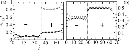
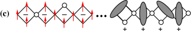
Figure 6: (Color online). GS properties at $\delta=0.18$ ($U=2$) and $\delta=0.28$ ($U=\infty$) for $N=100$ using DMRG. Expectation value of $n_{h,i}$ for (a) $U=2$ and (b) $U=\infty$. Effective linear chain notation:($\bullet$) identifies $A$ sites and ($\circ$) $B_{1}+B_{2}$ at the same cell. (c) Illustration of the GS for $U=\infty$ in the phase-separated regime: singlet bonds are represented by ellipses and holes by circles. $-$($+$) indicates odd (even) local parity. Dashed lines are guides to the eye.

At $\delta=1/3$, i. e., one hole per $A$ site for open BC’s using DMRG white , the GS has even parity and is fully dominated by the Mott insulating phase (even parity) illustrated in Fig. 6(c) for $U=\infty$. The charge gap $\Delta_{c}=\mu_{+}-\mu_{-}$, where $\mu_{+}=[E(N_{e}+\Delta N_{e})-E(N_{e})]/\Delta N_{e}$, $\Delta N_{e}>0$ ($\Delta N_{e}/N\rightarrow 0$), and $\mu_{-}=E(N_{e})-E(N_{e}-1)$, must be calculated with care. First, notice that adding electrons to $\delta=1/3$ places the system in the phase-separated (inhomogeneous) region where the chemical potential $\mu$ is flat. Indeed, by comparing results using DMRG and ED calculations for $U=\infty$, for which $\Delta_{c}$ presents little finite size corrections [Fig. 7(a)], we concluded that boundary effects are minimized by taking $\Delta N_{e}=2$ and placing the symmetry inverted cells at the chain center. We thus find [Fig. 7(a)] $\Delta_{c}\approx 0.21$ ($\approx 0.96$) for $U=2$ ($=\infty$). This problem is absent in the case of hole doping since the phase is homogeneous. The extrapolated spin gap,

$$\Delta_{S}=E(S=1)-E(S=0),$$ (12)

characterized by symmetry inversion of a cell at the chain center, is also shown in Fig. 7(a) for $U=2$ ($\Delta_{S}\approx 0.18$) and $U=\infty$ ($\Delta_{S}\approx 0.16$), with the spin gap at $U=\infty$ presenting little finite size dependence. It is a quite massive excitation with the magnon localized at the odd symmetry cell, mostly at the B sites, as shown in Fig. 7(b). In this context, Sierra et al. white found $\Delta_{S}\approx 0.27$ using the $t-J$ model ($J=4t^{2}/U$) for $J=0.35t$, i. e., $U\approx 11.43$. We have confirmed this result by studying the $U$ dependence of $\Delta_{S}$ using ED.

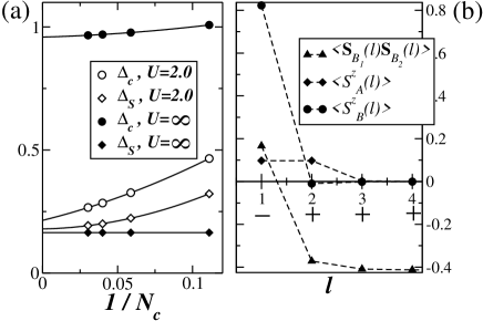
Figure 7: DMRG results for the (a) size dependence of the charge ($\Delta_{c}$) and spin ($\Delta_{S}$) gaps as function of $1/N_{c}$ at $\delta=1/3$: solid lines are polynomial fittings. ED results for the (b) expectation values of $S^{z}_{A}(l)$, $S^{z}_{B}(l)$ and the correlation function $\langle\mathbf{S}_{B_{1}}(l)\cdot\mathbf{S}_{B_{2}}(l)\rangle$ at spin sector $S^{z}=1$ as function of cell number $l$. The $\pm$ signs below the horizontal axis in (b) indicate the cell parity.

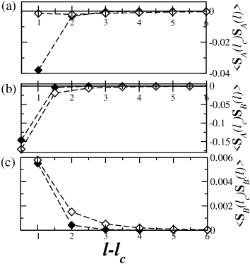
Figure 8: Spin correlation functions (a) $\langle\mathbf{S}_{A}(l_{c})\cdot\mathbf{S}_{A}(l)\rangle$, (b) $\langle\mathbf{S}_{A}(l_{c})\cdot\mathbf{S}_{B}(l)\rangle$ and (c) $\langle\mathbf{S}_{B}(l_{c})\cdot\mathbf{S}_{B}(l)\rangle$ as function of $l-l_{c}$ in the ELC at $\delta=1/3$ for $N_{c}=33$ using DMRG; in the above expressions $l_{c}$ denotes the central cell; ($\lozenge$) refers to $U=2$ and ($\blacklozenge$) to $U=\infty$. Dashed lines are guides to the eye. (d) Illustration of the GS at $\delta=1/3$, singlet bonds are represented by ellipses and holes by circles.

In Fig. 8 we show that the spin correlation functions at $\delta=1/3$, calculated using DMRG, present a fast decay and can be fitted with the exponential form $\exp{[-(l-l_{c})/\xi)]}$, where $\xi$ is the correlation length, $l$ is the cell index in the ELC and $l_{c}$ denotes the central cell of the system. This behavior is expected from the presence of a finite spin gap. The values of $\xi$ for the correlations $\langle\mathbf{S}_{A}(l_{c})\cdot\mathbf{S}_{A}(l)\rangle$, $\langle\mathbf{S}_{A}(l_{c})\cdot\mathbf{S}_{B}(l)\rangle$ and $\langle\mathbf{S}_{B}(l_{c})\cdot\mathbf{S}_{B}(l)\rangle$ are $\approx$ 0.4 (2.2), 0.25 (0.45) and 0.39 (0.75), respectively, for $U=\infty$ ($U=2$), with $l_{c}$ denoting the central cell. Thus, except for the correlation $\langle\mathbf{S}_{A}(l_{c})\cdot\mathbf{S}_{A}(l)\rangle$ at $U=2$, the correlation length is extremely short with spins correlated only within a cell. Further, the calculated bulk values of $\langle\mathbf{S}_{B_{1}}\cdot\mathbf{S}_{B_{2}}\rangle$ at $\delta=1/3$ are in very good agreement with those in the even phase of the separated region shown in Figs. 5(b) and 5(d). The above results support a short-range-RVB (SR-RVB) sr_rvb state for the GS at $\delta=1/3$, as illustrated in Fig. 8(d). In this context, Sierra et al. white reached similar conclusions using the $t-J$ model on the AB₂ chain, while Giesekus has proved giesekus that a SR-RVB state is the GS of a non-bipartite lattice with the same local symmetry but a different hopping pattern.

V Luttinger Liquid Behavior

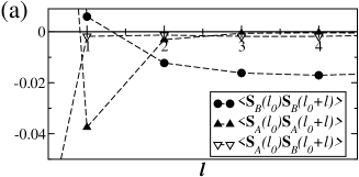
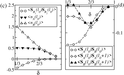
Figure 9: (a) ED results for the indicated spin correlation functions as function of cell index $l$, with $\mathbf{S}_{B}\equiv\mathbf{S}_{B_{1}}+\mathbf{S}_{B_{2}}$. (b) Illustration of the GS at $\delta=1/3$ doped with two holes: singlet bonds are represented by ellipses and holes by circles. (c) ED results for the spin correlation functions between $B$ sites at the same cell $\langle\mathbf{S}_{B_{1}}(l_{0})\cdot\mathbf{S}_{B_{2}}(l_{0})\rangle$, electron densities at $A$ sites $\langle n_{A}(l_{0})\rangle$ and at $B\equiv B_{1}+B_{2}$ sites $\langle n_{B}(l_{0})\rangle\equiv\langle n_{B_{1}}(l_{0})+n_{B_{2}}(l_{0})\rangle$. (d) ED results for the indicated nearest-neighbor spin correlation functions as function of $\delta$, with $\mathbf{S}_{B}\equiv\mathbf{S}_{B_{1}}+\mathbf{S}_{B_{2}}$. In (a), (c) and (d) $l_{0}$ denotes an arbitrary cell.

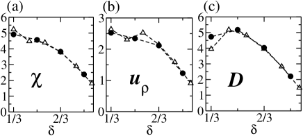
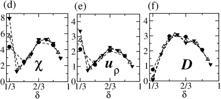
Figure 10: ED results for the charge susceptibility $\chi$, the charge excitation velocity $u_{\rho}$ and the Drude weight $D$, for $U=2$ [(a),(b) and (c)] and $U=\infty$ [(d), (e) and (f)], and $N_{c}=$ 4 ($\bullet$), 6 ($\triangle$) and 8 ($\blacktriangledown$).

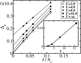
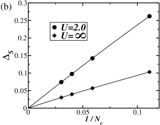
Figure 11: DMRG results for the (a) Charge gap $\Delta_{c}$ as function of $1/N_{c}$ at $\delta=2/3$ using DMRG; the inset presents extrapolated values of the charge gap as function of $U$ . DMRG calculation of the (b) Spin gap $\Delta_{S}$ as function of $1/N_{c}$ for $U=2$ ($\bullet$) and $U=\infty$ ($\blacklozenge$). Solid lines are polynomial fittings, except in the inset of (a), where we have used an essential singularity form as explained in the text.

We now focus on the behavior of the system for $1/3<\delta<1$ by considering a chain with closed boundary conditions and $N_{c}=8$ for $U=\infty$ using ED. The first noticeable feature is the behavior of the spin correlation functions after doping the $\delta=1/3$ GS with two holes. The value of $\langle\mathbf{S}_{B_{1}}(l_{0})\cdot\mathbf{S}_{B_{2}}(l_{0})\rangle$ (where $l_{0}$ denotes an arbitrary cell) changes from -0.41 to -0.28. This variation can be understood by considering that the two holes added to the system break two singlet bonds and reside predominately at B sites. In this picture the correlation function would amounts to $\frac{N_{c}-2}{N_{c}}(-0.41)\approx-0.31$, which is close to -0.28. Furthermore, the spin correlation functions shown in Fig. 9(a) evidence the formation of long ranged bonds between electrons on $B$ sites, while the other correlations remain short ranged, as in the $\delta=1/3$ ground state. This fact indicates that the electrons picked from the SR-RVB by hole doping are antiferromagnetically coupled and delocalized through the system, as illustrated in Fig. 9(b). In order to describe the system behavior for finite dopings, we display in Fig. 9(c) the correlation function $\langle\mathbf{S}_{B_{1}}(l_{0})\cdot\mathbf{S}_{B_{2}}(l_{0})\rangle$ and electronic densities as function of $\delta$. Notice that for $1/3<\delta<2/3$ the electronic density at $A$ sites is almost fixed, while that at $B$ sites are monotonically depopulated. As a consequence, $\langle\mathbf{S}_{B_{1}}(l_{0})\cdot\mathbf{S}_{B_{2}}(l_{0})\rangle$ continuously vanishes as the doping increases. Moreover, in Fig. 9(d) we show the relevant nearest-neighbor spin correlation functions. These correlations display quite different magnitudes at $\delta=1/3$, but their values approach each other for $\delta>2/3$. We thus consider the doping interval $1/3<\delta<2/3$ as a crossover region, where doping starts to build the Luttinger liquid which is fully established for $\delta>2/3$.

We have also calculated the charge compressibility $\kappa$ through

$$\chi=\frac{1}{n_{0}^{2}\kappa}=\frac{V}{4}[E(N_{e}+2)+E(N_{e}-2)-2E(N_{e})],$$ (13)

where $V$ is the volume and $n_{0}=\frac{N_{e}}{V}$ is the electronic density; the charge excitation velocity

$$u_{\rho}=\frac{E(\Delta k,S=0)-E_{GS}}{\Delta k},$$ (14)

with $\Delta k=2\pi/L$ and $L$ the system length; and the Drude weight

$$D=\frac{L}{4\pi}\left[\frac{\partial^{2}E(\Phi)}{\partial\Phi^{2}}\right]_{\Phi_{min}},$$ (15)

where $\Phi_{min}$ is the flux value that minimizes the energy fye . In an insulating phase these quantities satisfy the limits below

$$\lim_{N_{c}\rightarrow\infty}\left\{\begin{array}[]{ccc}\chi&=&\infty;\\ u_{\rho}&=&\infty;\\ D&=&0,\end{array}\right.$$ (16)

while for a metal $\chi$, $u_{\rho}$ and $D$ are finite. As shown in Fig. 10, at $\delta=1/3$, $\chi$ and $u_{\rho}$ increases, while $D$ decreases with system size for both $U=2$ and $U=\infty$, although the insulating character is better evidenced for $U=\infty$ due to its sizable charge gap, as shown in Fig. 7(a). At the other commensurate density, $\delta=2/3$, we can see the signals of an insulating phase for $U=\infty$, while for $U=2$ we does not observe any especial behavior. In order to clarify this point, we have used DMRG to study the size dependence of the charge gap for larger systems at this doping. For a finite open chain, the occupation of two holes per cell tends to $\delta=2/3$ in the thermodynamic limit. In Fig. 11(a), we can clearly observe that for $U=\infty$ the system is in a Mott insulating phase with $\Delta_{c}\approx 0.15$; however, the gap for $U=2$ is extremely small. In order to better understand the U-dependence of this gap, we have also calculated $\Delta_{c}$ for intermediate values of $U$, as also shown in Fig. 11(a). In the inset of Fig. 11(a) we have fit $\Delta_{c}(U)$ using an expression similar to the limiting behavior of the charge gap as $U\rightarrow 0$ of the Lieb-Wu solution for a linear chain at half filling liebwu : $U^{a}\exp{(-b/x)}$, in which $a\approx 0.61$ and $b\approx 7.95$ are fitting parameters. Notice, however, that contrary to the Lieb-Wu solution liebwu , $\Delta_{c}$ saturates to a finite value ($\approx 0.15$) for $U=\infty$. On the other hand, similarly to the linear chain at half filling liebwu , the data shown in Fig. 11(b) indicates the absence of spin gap at $\delta=2/3$ in the thermodynamic limit for both $U=2$ and $U=\infty$.

In the Luttinger model, it is well known luttinger that $\chi$, $u_{\rho}$ and $D$ are related through

$$D=2u_{\rho}K_{\rho},$$ (17)

with

$$K_{\rho}=\frac{\pi u_{\rho}}{2\chi},$$ (18)

where $K_{\rho}$ is the exponent governing the decay of the correlation functions. In order to probe the doped region for which the lower energy spectrum of the $AB_{2}$ chain can be mapped onto the Luttinger model, we consider the ratio

$$\mbox{Ratio}=\frac{u_{\rho}}{\sqrt{D\chi/\pi}},$$ (19)

which must be equal to one if the system is in the LL universality class poilblanc .

Since the $AB_{2}$ chain is not strictly one-dimensional, care must be taken with the length scales ($V$ and $L$) in Eqs. (13), (14) and (15). For $U=0$, the orbitals at sites $A$ and bonding orbitals at sites $B$ are translationally equivalent and both build the dispersive branches shown in Fig. 1(c). In this case, the system can be mapped onto a tight-binding linear chain with $2N_{c}$ sites and a rescaled hopping parameter, $t\rightarrow t\sqrt{2}$, with $K_{\rho}=1$. In order that Eq. (18) matches this result for $\epsilon_{F}<0$, we must choose $V\equiv L=2N_{c}$ with $\epsilon(k)=-2\sqrt{2}\cos(k)$; or, likewise, $V\equiv L=N_{c}$ and the dispersions as written in Eq. (3). In both cases $k_{F}=\frac{\pi}{2}n_{0}$, with $n_{0}=\frac{N_{e}}{L}$. Consider, for example, the former option. For $U=0$, the charge excitation velocity is equal to the Fermi velocity $u_{F}$, which can be easily calculated as

$$u_{F}=\left.\frac{\partial\epsilon(k)}{\partial k}\right|_{k=k_{F}}=2\sqrt{2}\sin(k_{F}).$$ (20)

On the other hand, substituting the GS energy,

$$E_{GS}(n_{0})=\frac{-8\sqrt{2}}{\pi}N_{c}\sin(\frac{\pi}{2}n_{0}),$$ (21)

into the continuous version of Eq. (13), we obtain,

$$\chi = \frac{1}{V}\frac{\partial^{2}E_{GS}}{\partial n_{0}^{2}},$$ (22)

$$= \pi\sqrt{2}\sin(\frac{\pi}{2}n_{0}).$$ (23)

Using now Eqs. (20) and (23) in Eq. (18) we find, as expected, $K_{\rho}=1$.

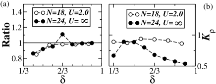
Figure 12: (a) ED results for the Ratio=$u_{\rho}/\sqrt{D\chi/\pi}$. (b) ED results for $K_{\rho}$ as function of $\delta$.

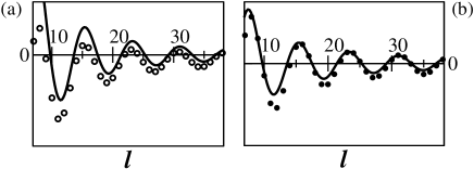
Figure 13: Spin correlation functions $C(l)$ for (a) $U=2$ and (b) $U=\infty$ at $\delta=88/106$ for $N=106$ using DMRG: solid lines are fittings using Eq. (25).

We now turn to the interacting case using ED. As shown in Fig. 12(a) the LL character is quite clear for $\delta>2/3$, while for $1/3<\delta<2/3$ we identify the crossover region. The ED results for $K_{\rho}$ are presented in Fig. 12(b). Notice that $K_{\rho}$ is close to 1 (non-interacting fermions) for $U=2$; while, $K_{\rho}$ is close to $1/2$ (non-interacting spinless fermions) for $U=\infty$ luttinger ; lluinf . In order to check these results, we used DMRG to calculate the ELC spin correlation function

$$C(l)\equiv\frac{\sum_{i,j}\langle\mathbf{S}_{i}\cdot\mathbf{S}_{j}\rangle\delta_{|i-j|,l}}{\sum_{i,j}\delta_{|i-j|,l}},$$ (24)

whose asymptotic behavior should match that for the Luttinger model lluinf :

$$C_{LL}(l)\sim\frac{\cos(2k_{F}l)[\ln(l)]^{1/2}}{l^{1+K_{\rho}}}.$$ (25)

In Eq. (24) we have considered an average over all possible pairs of sites separated by the same distance $l$, a procedure that reduces open boundary effects. In Figs. 13(a) and 13(b) we show $C(l)$ calculated at $\delta=88/106$ for $U=2$ and $U=\infty$, respectively. Also shown are the fittings to $C(l)$ using $C_{LL}(l)$ with $k_{F}=\frac{\pi}{2}n_{0}$ and $K_{\rho}$ taken from the results shown in Fig. 12(b) after linear interpolation: $K_{\rho}=0.89$ ($U=2$) and $K_{\rho}=0.57$ ($U=\infty$). Motivated by a compromise between large values of $l$ and minimum boundary effects, we have considered intermediate values of $l$ in the fitting, which is quite good for both values of $U$. We thus conclude that the Luttinger model correctly describes the low energy physics of the $AB_{2}$ chain for $\delta>2/3$.

VI Summary and Conclusions

In summary, the numerical results presented here have clearly evidenced the rich phase diagram exhibited by the Hubbard model on the doped AB₂ chain both for $U=2$ and in the infinite-U limit. We have shown that at the commensurate dopings $\delta=1/3$ and $2/3$ the system display insulating phases, although for $U=2$ the charge gap $\Delta_{c}$ is very small at $\delta=2/3$, with indications that $\Delta_{c}$ present an essential singularity as $U\rightarrow 0$. For $U=2$ and $\delta\lesssim 0.02$ the GS exhibit a ferrimagnetic phase reminiscent of the undoped regime, while for $0.02\lesssim\delta\lesssim 0.07$ incommensurate magnetic correlations are observed. For $U=\infty$ and $\delta=0$ the GS total spin is degenerate, whereas for $0<\delta\lesssim 0.225$ hole itinerancy (Nagaoka mechanism) sets a fully polarized GS. In this case, we have also observed the presence of an extensive number of low-lying levels with total spin ranging from the minimum value to $S_{max}-1$ and level spacing decaying with system size as $1/N_{c}$. For higher doping, the system phase separates into coexisting metallic and insulating phases for $\delta_{PS}(U)\lesssim\delta<1/3$ (with $\delta_{PS}(\infty)\approx 0.225$ and $\delta_{PS}(2)\approx 0.07$). The insulating state presents a finite spin gap and fully fills the system at $\delta=1/3$, which is well described by a short-ranged-RVB state. Finally, a crossover region is observed for $1/3<\delta<2/3$, while a Luttinger liquid behavior is explicitly characterized for $\delta>2/3$.

In closing, we would like to stress that the above-reported results might also stimulate further experimental and theoretical investigations on quasi-one-dimensional compounds displaying complex unit cell structures batista .

We acknowledge useful discussions with A. L. Malvezzi and M. H. Oliveira. This work was supported by CNPq, Finep, FACEPE and CAPES (Brazilian agencies).

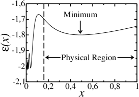
Figure 14: Energy per unit cell $\epsilon$ as function of the fraction $x=L_{-}/N_{c}$ for $\delta=0.28$. The physical region is also shown.

Appendix A Variational Approach for $U=\infty$ and $\delta\leq 1/3$

In the metallic saturated ferromagnetic region (parity symmetry -1) the energy as function of doping is known to have a non-interacting spinless fermion behavior:

$$E(k_{F-})=-\frac{4\sqrt{2}}{\pi}L_{-}\sin(k_{F-}/2),$$ (26)

where $k_{F-}=\pi\nu_{h-}$, $\nu_{h-}=N_{h-}/L_{-}$, and $L_{-}$ is the linear size of the system. On the other hand, in the insulating paramagnetic phase (SR-RVB states with even parity symmetry) at $\delta=1/3$ (one hole per cell)

$$N_{h+}=L_{+},$$ (27)

and the energy per cell $\epsilon_{+}$ is almost independent of the system linear size and can be estimated either by using ED or DMRG:

$$\epsilon_{+}\approx-2.021.$$ (28)

Let us now consider a phase-separated regime in which a paramagnetic phase with size $L_{+}$ coexists with a ferromagnetic one with size $L_{-}$, so the energy per cell reads

$$\epsilon=\epsilon_{+}\frac{L_{+}}{N_{c}}-\frac{4\sqrt{2}}{\pi}\frac{L_{-}}{N_{c}}\sin(\frac{\pi}{2}\nu_{h-}).$$ (29)

It is convenient to write $\nu_{h-}$ as

$$\nu_{h-}=\frac{N_{h}-(N_{c}-L_{-})}{L_{-}}=\frac{3\delta-(1-x)}{x}.$$ (30)

where $N_{h}=N_{h+}+N_{h-}$, $N_{c}=L_{+}+L_{-}$, $x=L_{-}/N_{c}$ and $N=3N_{c}$. Using the above notation we rewrite Eq. (29) in the form below

$$\epsilon(x)=(1-x)\epsilon_{+}-\frac{4\sqrt{2}}{\pi}x\sin\left[\frac{\pi}{2}\left(\frac{3\delta-1}{x}+1\right)\right]$$ (31)

Here we should notice the presence of a singularity at $x=0$ for any finite value of $\delta\neq 1/3$ (see Fig. 14). However, the region of physical values of $x$ is defined by

$$0\leq N_{h+}\leq N_{h},\mbox{ i. e.,}$$ (32)

$$1-3\delta\leq x\leq 1.$$ (33)

In Fig. 14 we present $\epsilon(x)$ for $\delta=0.28$, in which the physical region is $0.16\leq x\leq 1$ and can be found by Eq. (33), with a minimum in $\epsilon(x)$ for $x\approx 0.49$.

The value of $x$ which minimizes the energy for a given $\delta$, $\overline{x}=\overline{x}(\delta)$, satisfies the equation $\left[\frac{\partial\epsilon(x)}{\partial x}\right]_{\delta}=0$, which can be written as

$$\frac{\pi\epsilon_{+}}{4\sqrt{2}}=\cos(y)+y\sin(y),$$ (34)

where

$$y\equiv\frac{\pi}{2}\frac{3\delta-1}{\overline{x}}.$$ (35)

The roots of Eq. (34) are numerically calculated and conduct to

$$\left\{\begin{array}[]{lll}\overline{x}=1,&\mbox{for }&\delta\lesssim 0.225;\\ \overline{x}\approx 3.071-9.213\delta,&\mbox{for }&0.225\lesssim\delta\leq\frac{1}{3}.\end{array}\right.$$ (36)

We thus conclude that $\delta_{PS}(\infty)\approx 0.225$, which is in very good agreement with ED and DMRG calculations.

The magnetization is null at the even phase and maximum at the odd one. We can thus derive the following expression for the GS total spin per unit cell:

$$\frac{S_{g}}{N_{c}} = \frac{1}{2N_{c}}(N_{e}-2L_{+})$$ (37)

$$= \frac{1}{2}[3(1-\delta)-2(1-\overline{x})]$$ (38)

The dependence of the average parity $p$ on $\delta$ can also be easily written as

$$p=1-2\overline{x}$$ (39)

Finally, using Eq. (36) for $\overline{x}$, the above results for $p$ and $S_{g}$ are plotted in Figs. 2(d) and 3(c), respectively, and shown to be in excellent agreement with the ED and DMRG calculations.

References

- (1) P. W. Anderson, Science 235, 1196 (1987).
- (2) H. J. Schulz, Phys. Rev. Lett. 64, 1445 (1990); B. M. Andersen and P. Hedegard, Phys. Rev. Lett. 95, 037002 (2005).
- (3) Y. Nagaoka, Phys. Rev. 147, 392 (1966);
- (4) H. Tasaki, Prog. of Theor. Phys. 99, 489 (1998) and references therein, including those describing the occurrence of flat band, or nearly flat band, saturated ferromagnetism at finite .
- (5) Saturated ferromagnetism in the square lattice was recently showed to occur in the infinite-U limit and a unit flux quantum per electron: Y. Saiga and M. Oshikawa, Phys. Rev. Lett. 96, 036406 (2006).
- (6) P. W. Anderson, The Theory of Superconductivity in the High-Tc Cuprates (Princeton UniversityPress, Princeton, 1997).
- (7) V. J. Emery, S. A. Kivelson, and H. Q. Lin, Phys. Rev. Lett. 64, 475 (1990).
- (8) E. Dagotto, Science 309, 257 (2005).
- (9) F. D. M. Haldane, J. Phys. C 14, 2585 (1981); J. Voit, Rep. Prog. Phys. 58, 977 (1995).
- (10) A. M. S. Macêdo, M. C. dos Santos, M. D. Coutinho-Filho, and C. A. Macêdo, Phys. Rev. Lett. 74, 1851 (1995).
- (11) G. Sierra, M. A. Martín-Delgado, S. R. White, D. J. Scalapino, and J. Dukelsky, Phys. Rev. B 59, 7973 (1999).
- (12) Y. Watanabe and S. Miyashita, J. Phys. Soc. Jpn. 68, 3086 (1999).
- (13) M. A. Martín-Delgado, J. Rodriguez-Laguna, and G. Sierra, Phys. Rev. B 72, 104435 (2005).
- (14) G.-S. Tian and T.-H. Lin, Phys. Rev. B 53, 8196 (1996).
- (15) C. P. de Melo and S. A. F. Azevedo, Phys. Rev. B 53, 16258 (1996).
- (16) Y. F. Duan and K. L. Yao, Phys. Rev. B 63, 134434 (2001); W. Z. Wang, B. Hu, and K. L. Yao, Phys. Rev. B 66, 085101 (2002).
- (17) R. R. Montenegro-Filho and M. D. Coutinho-Filho, Physica A 357, 173 (2005).
- (18) T. Nakanishi and S. Yamamoto, Phys. Rev. B 65, 214418 (2002); C. Vitoriano, F. B. de Brito, E. P. Raposo, and M. D. Coutinho-Filho, Mol. Cryst. Liq. Cryst. 374, 185 (2002).
- (19) F. C. Alcaraz and A. L. Malvezzi, J. Phys. A: Math. Gen. 30, 767 (1997).
- (20) E. P. Raposo and M. D. Coutinho-Filho, Phys. Rev. Lett. 78, 4853 (1997); Phys. Rev. B 59, 14384 (1999).
- (21) M. H. Oliveira, M. D. Coutinho-Filho and E. P. Raposo, Phys. Rev. B 72, 214420 (2005).
- (22) C. Vitoriano, M. D. Coutinho-Filho and E. P. Raposo, J. Phys. A: Math. Gen. 35, 9049 (2002).
- (23) J. B. Anderson, E. Kostiner, and F. A. Ruszala, J. Solid State Chem. 39, 29 (1981).
- (24) M. Drillon, M. Belaiche, P. Legoll, J. Aride, A. Boukhari, and A. Moqine, J. Magn. Magn. Mater. 128, 83 (1993).
- (25) A. A. Belik, A. Matsuo, M. Azuma, K. Kindo, and M. Takano, J. Solid State Chem. 178, 709 (2005).
- (26) M. Matsuda, K. Kakurai, A. A. Belik, M. Azuma, M. Takano, and M. Fujita, Phys. Rev. B 71, 144411 (2005).
- (27) A. Boukhari, A. Moqine, and S. Flandrois, Mat. Res. Bull. 21, 395 (1986).
- (28) H. Effenberger, J. Solid State Chem. 142, 6 (1999).
- (29) M. Verdaguer, M. Julve, A. Michalowicz, and O. Kahn, Inorg. Chem. 22, 2624 (1983); Y. Pei, M. Verdaguer, O. Kahn, J. Sletten, and J.-P. Renard, Inorg. Chem. 26, 138 (1987); P. J. van Koningsbruggen, O. Kahn, K. Nakatani, Y. Pei, J. P. Renard, M. Drillon, and P. Legoll, Inorg. Chem. 29, 3325 (1990).
- (30) S. K. Pati, S. Ramasesha, and D. Sen, Phys. Rev. B 69, 8894 (1997); S. Yamamoto, S. Brehmer and H.-J. Mikeska, Phys. Rev. B 57, 13610 (1998); N. B. Ivanov, Phys. Rev. B 62, 3271 (2000); S. Yamamoto, Phys. Rev. B 69, 064426 (2004) and references therein.
- (31) Y. Hosokoshi, K. Katoh, Y. Nakazawa, H. Nakano, and K. Inoue, J. Am. Chem. Soc. 123, 7921 (2001); K. L. Yao, Q. M. Liu, and Z. L. Liu, Phys. Rev. B 70, 224430 (2004); K. L. Yao, H. H. Fu, and Z. L. Liu, Solid State Commun. 135, 197 (2005).
- (32) S. A. Kivelson, I. P. Bindloss, E. Fradkin, V. Oganesyan, J. M. Tranquada, A. Kapitulnik and C. Howald, Rev. Mod. Phys. 75, 1201 (2003).
- (33) E. H. Lieb, Phys. Rev. Lett. 62, 1201 (1989).
- (34) S. R. White, Phys. Rev. B 48, 10345 (1993); U. Schollwöck, Rev. Mod. Phys. 77, 259 (2005).
- (35) R. Jullien and R. M. Martin, Phys. Rev. B 26, 6173 (1982).
- (36) Raffaele Resta and Sandro Sorella, Phys. Rev. Lett. 82, 2560 (1999); A. A. Aligia and G. Ortiz, Phys. Rev. Lett. 82, 370 (1999).
- (37) S. Liang and H. Pang, Europhys. Lett. 32, 173 (1995); M. Kohno, Phys. Rev. B 56, 15015 (1997); H. Ueda and T. Idogaki, Phys. Rev. B 69, 104424 (2004).
- (38) M. Troyer, H. Tsunetsugu, and T. M. Rice, Phys. Rev. B 53, 251 (1996).
- (39) F. Becca and S. Sorella, Phys. Rev. Lett. 86, 3396 (2001).
- (40) K. Kusakabe and H. Aoki, Phys. Rev. B 52, R8684 (1995).
- (41) T. Koma and H. Tasaki, J. Stat. Phys. 76, 745 (1994); R. Arita and H. Aoki, Phys. Rev. B 61, 12261 (2000).
- (42) S. R. White and D. J. Scalapino, Phys. Rev. B 61, 6320 (2000).
- (43) E. Eisenberg, R. Berkovits, David A. Huse, and B. L. Altshuler, Phys. Rev. B 65, 134437 (2002).
- (44) D. S. Rokhsar and S. A. Kivelson, Phys. Rev. Lett. 61, 2376 (1988).
- (45) A. Giesekus, Phys. Rev. B 52, 2476 (1995).
- (46) R. M. Fye, M. J. Martins, D. J. Scalapino, J. Wagner, and W. Hanke, Phys. Rev. B 44, 6909 (1991).
- (47) E. H. Lieb and F. Y. Wu, Phys. Rev. Lett. 20, 1445 (1968).
- (48) see, e. g., C. A. Hayward and D. Poilblanc, Phys. Rev B 53, 11721 (1996).
- (49) A. Parola and S. Sorella, Phys. Rev. Lett. 64, 1831 (1990); H. J. Schulz, Phys. Rev. Lett. 64, 2831 (1990).
- (50) C. D. Batista and B. S. Shastry, Phys. Rev. Lett. 91, 116401 (2003).