Intrinsic and extrinsic noise effects on the phase transition of swarming systems and related network models

Abstract

We analyze order-disorder phase transitions driven by noise that occur in two kinds of network models closely related to the self-propelled model proposed by Vicsek et. al. to describe the collective motion of groups of organisms [Phys. Rev. Lett. 75:1226 (1995)]. Two different types of noise, which we call intrinsic and extrinsic, are considered. The intrinsic noise, the one used by Vicsek et. al. in their original work, is related to the decision mechanism through which the particles update their positions. In contrast, the extrinsic noise, later introduced by Grégoire and Chaté [Phys. Rev. Lett. 92:025702 (2004)], affects the signal that the particles receive from the environment. The network models presented here can be considered as the mean-field representation of the self-propelled model. We show analytically and numerically that, for these two network models, the phase transitions driven by the intrinsic noise are continuous, whereas the extrinsic noise produces discontinuous phase transitions. This is true even for the small-world topology, which induces strong spatial correlations between the network elements. We also analyze the case where both types of noise are present simultaneously. In this situation, the phase transition can be continuous or discontinuous depending upon the amplitude of each type of noise.

I Introduction

In spite of many efforts, only a limited understanding has been achieved regarding the emergence of collective order in non-equilibrium systems. While these systems often present features analogous to the those found in equilibrium, such as phase-transitions and long-range correlations, it is not clear how to use the powerful tools available in equilibrium statistical mechanics to analyze their properties. To overcome this problem, it may be useful to consider cases where simple qualitative characteristics (e.g. the existence and order of a phase transition) are common to different non-equilibrium systems with similar properties.

A class of non-equilibrium systems that has sparked increasing interest in recent years is given by models of groups of swarming agents Grunbaum ; Vicsek ; Czirok1 ; Czirok2 ; Nagy ; Topaz1 . These are used to describe the collective behavior of self-propelled agents such as schools of fish, flocks of birds, or herds of quadrupeds Parrish ; Couzin1 ; Couzin2 . Even the simplest of these models displays large-scale organized structures, in which agents separated by distances much larger than their interaction ranges can coordinate and swarm in the same direction. If noise is added to the system, this ordered state is destroyed as the noise level increases. When the noise reaches a critical value, the system undergoes a phase transition to a disordered state where agents move in random directions Vicsek ; Czirok1 . This phase transition has been quite thoroughly analyzed through numerical simulations. However, the lack of a systematic theoretical approach to non-equilibrium systems has hindered a proper characterization of the order-disorder phase transition, and there are still doubts about its basic features even in this simplest of cases Chate ; OurPRL ; ChateComment .

In this paper we are particularly interested in how this phase transition might be affected by the way in which the noise is introduced in the system. Two different types of noise, which we will call extrinsic and intrinsic, have recently been considered in models of swarming Vicsek ; Chate . In these models, at every time step each particle receives a signal from its neighbors that tells the particle in which direction to move next. The extrinsic noise consists in that the signal received by the particle is blurred (because, say, the environment is not completely transparent and the particle cannot see its neighbors very well). As a consequence, the particle may move in a different direction to the one dictated by the neighbors. In contrast, in the intrinsic noise case each particle receives the signal sent by the neighbors perfectly, but then it may “decide” to do something else and move in a different direction. Thus, the extrinsic noise can be thought of as produced by a blurry environment, whereas the intrinsic noise comes from the “free will” of the particles, so to speak; namely, from the uncertainty in the particle’s decision mechanism. In either case, of course, the net result is that, at every time step, the particle may move in a direction that departs from the one dictated by the neighbors.

It has been pointed out that these two distinct types of noise, extrinsic and intrinsic, can produce very different order-disorder phase transitions OurPRL . This can been shown analytically using a network approach in which the elements, instead of interacting with the neighbors in a physical space, interact with any element that is linked to them through a network connection. This kind of description has been used to model a large range of dynamics, such as the traffic between Internet websites or servers, the evolution of an epidemic outbreak, the mechanisms triggered by gene expressions in the cell, or the activity of the brain Barabasi1 ; Strogatz ; Watts3 ; Watts4 ; ReviewBarabasi ; ReviewNewman . In the context of swarming systems, the network approach is equivalent to a mean-field theory in which correlations between the particles are not taken into account. However, this approach has the virtue that it allows us to separate clearly the dynamical interaction rule that determines the dynamical state of the particles, from the topology of the underlying network that develops in time and space and dictates who interacts with who. Therefore, under the network approach it is possible to focus on the effects that the two different types of noise have on the dynamics of the system.

Even when the network approach leaves aside some important aspects of the dynamics of swarming systems (such as correlations in space and time), some appealing analogies can be established between the swarming and network systems. Indeed, in the simplest swarming models, the dynamics is defined by giving to each agent a steering rule that uses the velocities of all agents in its vicinity as an input to compute its own velocity for the next time-step. This algorithm can be associated to a dynamics on a switching network that links at every time-step all agents that are within the interaction range of each other. In this context, the network is simply a representation of the spatial dynamics of the system. However, it has been shown that this analogy can be pushed further successfully and that a static network with long-range connections can capture some of the main qualitative behaviors of simple swarming models Huepe1 ; Aldana1 ; OurPRL .

In this paper, we compare the properties of the phase transitions and dynamical mappings of two kinds of network models to further explore the analogies described above. We consider models that incorporate three of the main aspects of the interaction between the particles in swarms: an average input signal from the neighbors, noise, and, in some sense, extremely long-range interactions. In the first kind of model the elements of the network can acquire only two states, +1 and -1; whereas in the second, the elements are represented by 2D vectors whose angles take any value between 0 and $2\pi$. We find that swarming systems and their network counterparts indeed present qualitatively similar behaviors depending on whether the noise is intrinsic or extrinsic. We also determine numerically that the same qualitative features arise when the particles are placed on a small-world network, and we extend our results to the case in which the network models are subject to both types of noise.

The paper is organized as follows. In Sec. II we present the model introduced by Vicsek and his group to describe the emergence of order in swarming systems. In particular, we focus our attention on how the phase transition seems to change when the noise changes from intrinsic to extrinsic. In Section III we present a majority voter model on a network, which is reminiscent of the Ising model with discrete internal degrees of freedom. This model is simple enough as to be treated analytically, at least for the case of homogeneous random network topologies for which we show analytically that the two types of noise indeed produce two different types of phase transition. In Sec. IV we introduce another network model in which the internal degrees of freedom are continuous (2D vectors). This model can be treated analytically in the limit of infinite network connectivity. However, these results and extensive numerical simulations clearly indicate that the two types of noise again produce two different phase transitions, which are analogous to the ones observed in the majority voter model and in the self-propelled model. In Sec. V we discuss the mean-field assumptions conveyed in the two network models and how they relate to the self-propelled model. We also show that the nature of the phase transition produced by each type of noise does not change when the small-world topology is implemented, which produces strong spatial correlations between the network elements. Finally, in Section VI we summarize our results.

II The Vicsek model

Arguably, the simplest model to describe the collective motion of a group of organisms was proposed by Vicsek and his collaborators Vicsek . In this model, $N$ particles move within a 2D box of sides $L$ with periodic boundary conditions. The particles are characterized by their positions, $\vec{x}_{1}(t),\dots,\vec{x}_{N}(t)$, and their velocities $\vec{v}_{1}(t)=ve^{i\theta_{1}(t)},\dots,\vec{v}_{N}(t)=ve^{i\theta_{N}(t)}$, (represented here as complex numbers). All the particles move with the same speed $v$. However, the direction of motion $\theta_{n}(t)$ of each particle changes in time according to a rule that captures in a qualitative way the interactions between organisms in a flock. The basic idea is that each particle moves in the average direction of motion of the particles surrounding it, plus some noise. Two interaction rules have been considered in the literature, which differ in the way the noise is introduced into the system. To state these rules mathematically, we need some definitions. Let ${\mathcal{R}}_{n}(r)$ be the circular vicinity of radius $r$ centered at $\vec{x}_{n}(t)$, and $K_{n}(t)$ be the number of particles whose positions are within ${\mathcal{R}}_{n}(r)$ at time $t$. We will denote as $\vec{U}_{n}(t)$ the average velocity of the particles which at time $t$ are within the vicinity ${\mathcal{R}}_{n}(r)$, namely

$$\vec{U}_{n}(t)=\frac{1}{K_{n}(t)}\sum_{\{j\,:\,\vec{x}_{j}(t)\in{\mathcal{R}}_{n}(r)\}}\vec{v}_{j}(t).$$ (1)

For reasons that will be clear later, we will call $\vec{U}_{n}(t)$ the input signal received by the $n$-th particle $\vec{v}_{n}$. With the above definitions, the interaction rule originally proposed by Vicsek et al. can be written as

$$\theta_{n}(t+\Delta t) = \mbox{Angle}\left[\vec{U}_{n}(t)\right]+\eta\xi_{n}(t),$$ (2a)

$$\vec{v}_{n}(t+\Delta t) = ve^{i\theta_{n}(t+\Delta t)},$$ (2b)

$$\vec{x}_{n}(t+\Delta t) = \vec{x}_{n}(t)+\vec{v}_{n}(t+\Delta t)\Delta t,$$ (2c)

where $\xi_{n}(t)$ is a random variable uniformly distributed in the interval $[-\pi,\pi]$, and the noise amplitude $\eta$ is a parameter taking a constant value in $[0,1]$. The “Angle” function is defined in such a way that if $\vec{u}=ue^{i\theta}$, then Angle$[\vec{u}]=\theta$. Note that in this case the direction of the neighbors’ average velocity $\vec{U}_{n}(t)$ (the input signal) is computed first and then the noise is added to this direction. We will refer to the interaction rule given in Eqs. (2) as the self-propelled model with intrinsic noise (SPMIN), and to the term $\eta\xi_{n}(t)$ as the intrinsic noise.

The second interaction rule, proposed by Grégoire and Chaté in Ref. Chate , is given by

$$\theta_{n}(t+\Delta t) = \mbox{Angle}\left[\vec{U}_{n}(t)+\eta e^{i\xi_{n}(t)}\right],$$ (3a)

$$\vec{v}_{n}(t+\Delta t) = ve^{i\theta_{n}(t+\Delta t)},$$ (3b)

$$\vec{x}_{n}(t+\Delta t) = \vec{x}_{n}(t)+\vec{v}_{n}(t+\Delta t)\Delta t,$$ (3c)

where $\xi_{n}(t)$ and $\eta$ have the same meaning as in Eq. (2a). In this case, a random vector of constant length $\eta$ and random orientation $\xi_{n}(t)$ is added to the neighbors’ average velocity $\vec{U}_{n}(t)$, and then the direction of the resultant vector is computed. We will refer to the model given in Eqs. (3) as the self-propelled model with extrinsic noise (SPMEN), and to the term $\eta e^{i\xi_{n}(t)}$ as the extrinsic noise.

One might think that the two interaction rules (2a) and (3a) are more or less equivalent and should produce qualitatively similar dynamical behaviors. However, as mentioned in the introduction, there is a clear physical difference between these two ways of adding noise to the system. In the SPMIN the uncertainty induced by the noise is in the decision mechanism (the Angle function), but not in the input signal that each particle receives. In contrast, one could say that in the SPMEN the particles are “short-sighted” and do not see well the signal sent by the neighbors, which is what causes the uncertainty in this case. Thus, one cannot expect, a priori, the onset of collective order to be the same in both the SPMIN and the SPMEN, for the way in which the noise is introduced in both cases is clearly different, not only algorithmically, but also physically.

To measure the amount of order in the system we define the instantaneous value of the order parameter $\psi(t)$ as

$$\psi(t)=\left|\frac{1}{vN}\sum_{n=1}^{N}\vec{v}_{n}(t)\right|=v^{-1}\left|\langle\vec{U}(t)\rangle\right|,$$ (4)

where $\langle\vec{U}(t)\rangle=\frac{1}{N}\sum_{n=1}^{N}\vec{v}_{n}(t)$ is the average velocity of the entire system at time $t$. Thus, if $\psi(t)\approx 0$ the particles move in random uncorrelated directions, whereas if $\psi(t)\approx 1$, all the particles are aligned and move in the same direction. In the limit $t\to\infty$, the order parameter $\psi(t)$ reaches a constant value $\psi=\lim_{t\to\infty}\psi(t)$ that characterizes the steady state behavior of the system .

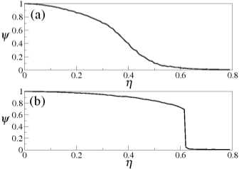
Figure 1: Phase transition in the self-propelled model with (a) intrinsic noise and (b) extrinsic noise. In the first case the phase transition seems to be continuous, whereas in the second case it is clearly discontinuous. The numerical simulations were performed using systems with $N=20000$, $L=32$, $r=0.4$ and $v=0.05$.

In their original work, Vicsek and his group noted the existence of a phase transition from ordered states ($\psi(t)>0$) to disordered states ($\psi(t)\approx 0$) as the value of the noise intensity $\eta$ increases. We illustrate this phase transition for the SPMIN in Fig. 1(a), which was obtained numerically for a system with $N=20000$ particles within a box of sides $L=32$. The interaction radius and particle speed used in the numerical simulation are $r=0.4$ and $v=0.05$, respectively. On the other hand, Fig. 1(b) shows the phase transition for the SPMEN with exactly the same parameters as in the previous case. As it can be seen from Fig. 1, the phase transition looks continuous (second order) for the SPMIN, whereas it is clearly discontinuous (first order) for the SPMEN.

Numerical simulations performed for larger systems than the one used in Fig. 1 also seem to indicate that the phase transition exhibited in the SPMIN is continuous Czirok1 ; Czirok2 ; Nagy . Nonetheless, based on numerical simulations, the authors of Ref. Chate have pointed out that the phase transition may be discontinuous regardless of the type of noise, and that the apparent continuity of the phase transition in the SPMIN is due to strong finite-size effects. For some reason, these finite size effects are not so strong in the SPMEN, in which the phase transition is clearly discontinuous. Due to a lack of a general mathematical formalism to analyze the self-propelled model, (either with intrinsic or extrinsic noise), the way in which each type of noise affects the dynamics of the system remains unknown. In what follows we present two simplified versions of the Vicsek model that can be solved analytically for the two types of noise. We show that in these simpler models, the phase transition is continuous for the intrinsic noise and discontinuous for the extrinsic noise.

III The majority voter model

The first network model that we consider consists of a set of $N$ binary variables, $v_{1},v_{2},\dots,v_{N}$, each acquiring the values +1 or -1. The value of each $v_{n}$ changes in time and is determined by a set of $k_{n}$ other elements, ${\mathcal{I}}_{n}=\{v_{n_{1}},v_{n_{2}},\dots,v_{n_{k_{n}}}\}$, which we will call the inputs of $v_{n}$. Thus, at every time step every element $v_{n}$ receives a signal from its set of inputs ${\mathcal{I}}_{n}$ and updates its value according to that signal. Different ways of assigning the inputs to each element lead to different network topologies. In this section we focus on the homogeneous random topology characterized by the following two properties:

• All the elements have the same number of inputs $K$, namely, $k_{n}=K$ for all $n$.

• The $K$ inputs of each element are chosen randomly from anywhere in the system.

Note that this is a directed network, for if $v_{n}$ is an input to $v_{m}$, then $v_{m}$ is not necessarily an input to $v_{n}$. We can think of this system as a society of $N$ individuals in which every individual $v_{n}$ can have two opinions (+1 and -1) about an issue. Each individual’s opinion is influenced by its $K$ friends (inputs), who are randomly chosen among the $N$ individuals in the society. Generally, each individual will tend to be of the same opinion as the majority of its friends, but with a given probability it can have the opposite opinion. This probability of having an opinion opposite to that of the majority can be considered as a “temperature” that introduces noise in the dynamics of the system. Here we consider two ways of introducing this noise, which are analogous to the intrinsic and extrinsic noise in the self-propelled model.

We define the input signal $U_{n}(t)$ influencing element $v_{n}(t)$ as

$$U_{n}(t)=\frac{1}{K}\sum_{j=1}^{K}v_{n_{j}}(t).$$ (5)

This is just the average opinion of the inputs of $v_{n}$. With this definition, the dynamics of the system with intrinsic noise is given by the simultaneous updating of the network elements according to the rule

$$v_{n}(t+1)=\left\{\begin{array}[]{rll}\mbox{Sign}\left[U_{n}(t)\right]&\mbox{ with prob. }&1-\eta\\ &&\\ -\mbox{Sign}\left[U_{n}(t)\right]&\mbox{ with prob. }&\eta\\ \end{array}\right.$$ (6)

where Sign$[U_{n}]=-1$ if $U_{n}<0$, and Sign$[U_{n}]=1$ if $U_{n}>0$. If $U_{n}=0$ then we choose for $v_{n}(t+1)$ either +1 or -1 with equal probability. The noise amplitude $\eta$ is a constant parameter in the interval $[0,1/2]$ that represents the probability for each individual to go against the majoritarian opinion. The above interaction rule can also be written in a simpler form as

$$v_{n}(t+1)=\mbox{Sign}\left[\mbox{Sign}\left[U_{n}(t)\right]+\frac{\xi_{n}(t)}{1-\eta}\right],$$ (7)

where $\xi_{n}(t)$ is a random variable uniformly distributed in the interval $[-1,1]$. From the above expression it is clear that this way of introducing the noise is equivalent to the intrinsic noise of Eq. (2a), since the noise is added after the Sign function has been applied to the input signal $U_{n}(t)$. (Since $v_{n}$ can only take the values +1 or -1, the Sign function has to be applied again.)

The other way of introducing the noise, which is equivalent to the extrinsic noise in Eq. (3a), is given by the interaction rule

$$v_{n}(t+1)=\mbox{Sign}\left[U_{n}(t)+4\eta\xi_{n}(t)\right],$$ (8)

where now the noise is directly added to the input signal $U_{n}(t)$ and then the Sign function is evaluated. $\xi_{n}(t)$ and $\eta$ have the same meaning as in Eq.  (7). (The factor 4 in the preceding equation is just to guarantee that the phase transition in this case occurs within the interval $\eta\in[0,1/2]$.)

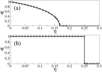
Figure 2: Phase transition in the majority voter model with (a) intrinsic noise and (b) extrinsic noise. In the first case the phase transition is continuous, whereas in the second case it is discontinuous. The symbols represent data obtained from numerical simulations using systems with $N=10^{5}$ and $K=3$. The solid lines correspond to the mean-field prediction.

For both types of noise, intrinsic and extrinsic, the majority voter model exhibits a phase transition from ordered to disordered states. However, the nature of this phase transition (i.e. whether continuous or discontinuous) depends on the type of noise. To see that this is indeed the case, we define the order parameter $\psi(t)$ for the majority voter model as

$$\psi(t)=\frac{1}{N}\sum_{n=1}^{N}v_{n}(t).$$ (9)

In the limit $t\to\infty$, the order parameter $\psi(t)$ reaches a stationary value $\psi$ that depends on the noise intensity $\eta$. Fig. 2(a) shows $|\psi|$ as a function of $\eta$ for the intrinsic noise case [Eq. (7)], in a system with $N=10^{5}$ and $K=3$. It is apparent that in this case the phase transition is continuous. This result is consistent with the behavior of the SPMIN reported in Fig. 1(a). Contrary to the above, the phase transition for the majority voter model with extrinsic noise [Eq. (8)] is discontinuous, as is shown in Fig. 2(b), which is also consistent with the behavior observed in Fig. 1(b) for the SPMEN. Thus, changing the way in which the noise is introduced in the voter model also changes drastically the nature of the phase transition.

The majority voter model is simple enough to be treated analytically. We can even generalize the model to incorporate the two types of noise simultaneously. In this generalization, the value of each element $v_{n}$ is updated according to the dynamical rule

$$v_{n}(t+1)=\mbox{Sign}\left[\mbox{Sign}\left[U_{n}(t)+4\eta_{1}\xi_{n}(t)\right]+\frac{\zeta_{n}(t)}{1-\eta_{2}}\right],$$ (10)

where $\xi_{n}$ and $\zeta_{n}$ are independent random variables uniformly distributed in the interval $[-1,1]$, and $\eta_{1}$ and $\eta_{2}$ are constant parameters taking values in the interval $[0,1/2]$. Thus, if $\eta_{1}=0$ and $\eta_{2}\neq 0$, only the intrinsic noise is present, whereas if $\eta_{1}\neq 0$ and $\eta_{2}=0$ only the extrinsic noise is present. Intermediate cases are obtained if both $\eta_{1}$ and $\eta_{2}$ are different from zero. In what follows we consider separately the case in which $K$ is finite, and the case in which $K$ is infinite.

III.1 Case 1: $K<\infty$

In Appendix A we present a mean-field calculation showing that, when the network connectivity $K$ is finite, the order parameter $\psi(t)$ satisfies the dynamical mapping

$$\psi(t+1)=M\left(\psi(t)\right),$$ (11a)

where

$$M(\psi)=(1-2\eta_{2})\sum_{m=1}^{K}\beta_{m}^{K}(\eta_{1})\psi^{m},$$ (11b)

and the coefficients $$\beta_{m}^{K}(\eta_{1})$$ are given by

$$\beta_{m}^{K}(\eta_{1}) = \binom{K}{m}\frac{(-i)^{m-1}}{4\pi K\eta_{1}}$$ (11c)

$$\times \int_{-\infty}^{\infty}\left[\cos\lambda\right]^{K-m}\left[\sin\lambda\right]^{m}\frac{\sin(4K\eta_{1}\lambda)}{\lambda^{2}}d\lambda.\ \ \$$

In the calculations that leads to the set of equations (11) one assumes that the network elements $v_{n}$ are statistically independent and equivalent (see Appendix A). These assumptions hold as long as the $K$ inputs of each element are chosen randomly from anywhere in the system, namely, for the homogeneous random topology. For other topologies that introduce correlations between the network elements, such as the small-world or the scale-free topologies, the mean-field assumptions do not necessarily apply. However, when they do apply, the order parameter given in Eq. (9) becomes the sum of $N$ independent and equally distributed random variables. Therefore, the determination of $\psi(t)$ becomes analogous to determining the average position of a 1D biased random walk, which can be solved exactly.

The stable fixed points of Eq. (11a) give the stationary values $\psi=\lim_{t\to\infty}\psi(t)$ of the order parameter. It is clear from Eqs. (11) that $\psi=0$ is always a fixed point. However, its stability depends on the values of $\eta_{1}$ and $\eta_{2}$. Additionally, from Eq. (11c) it follows that $\beta_{m}^{K}(\eta_{1})=0$ for even values of $m$ (because in such a case the integrand in that equation is an odd function). Therefore, the polynomial in Eq. (11b) contains only odd powers of $\psi(t)$ and thus, for each fixed point $\psi$, the opposite value $-\psi$ is also a fixed point.

To illustrate the formalism, we present here a detailed analysis of the simple case $K=3$. However, the results are similar for any other finite value of $K$. For $K=3$, the integrals in Eq. (11c) can be easily computed (we used Mathematica wolfram ) and Eq. (11b) becomes

$$M(\psi)=(1-2\eta_{2})\Big{(}\beta_{1}^{3}(\eta_{1})\psi+\beta_{3}^{3}(\eta_{1})\psi^{3}\Big{)},$$ (12a)

where

$$\beta_{1}^{3}(\eta_{1}) = \frac{4+24\eta_{1}-|1-12\eta_{1}|-3|1-4\eta_{1}|}{32\eta_{1}},$$ (12b)

$$\beta_{3}^{3}(\eta_{1}) = -\frac{8\eta_{1}-|1-12\eta_{1}|+|1-4\eta_{1}|}{32\eta_{1}}.$$ (12c)

To determine the stability of the fixed points of the mapping $M(\psi)$ we have to analyze the value of the derivative $M^{\prime}(\psi)\equiv dM(\psi)/d\psi$. If $|M^{\prime}(\psi)|<1$ at the fixed point, then that fixed point is stable. Otherwise, it is unstable. We further divide our presentation in three cases.

III.1.1 Sub-case 1: $\eta_{2}=0$

Let us first show that the phase transition is discontinuous for the case in which $\eta_{2}=0$, namely, when there is no intrinsic noise and only the extrinsic noise is present. Under these circumstances, the fixed-point equation $\psi=M(\psi)$ becomes

$$\psi=M(\psi)=\beta_{1}^{3}(\eta_{1})\psi+\beta_{3}^{3}(\eta_{1})\psi^{3}.$$ (13)

Using Eqs. (12b) and (12c), it is easy to see that $\psi=1$ and $\psi=-1$ are solutions of the fixed-point equation (13) provided that $0\leq\eta_{1}<\frac{1}{4}$ (in addition to the trivial solution $\psi=0$ which is always a fixed point). From Eqs. (12b), (12c) and (13) we obtain that

$$M^{\prime}(1) = \beta_{1}^{3}(\eta)+3\beta_{3}^{3}(\eta_{1})$$

$$= \left\{\begin{array}[]{lll}0&\mbox{ if }&0\leq\eta_{1}\leq\frac{1}{12}\\ &&\\ \frac{12\eta_{1}-1}{8\eta_{1}}&\mbox{ if }&\frac{1}{12}\leq\eta_{1}\leq\frac{1}{4}\\ &&\\ \frac{1}{4\eta_{1}}&\mbox{ if }&\frac{1}{4}\leq\eta_{1}\end{array}\right.$$

It follows from the above expression that $|M^{\prime}(\pm 1)|<1$ in the region $0\leq\eta_{1}<\frac{1}{4}$, which shows that the fixed points $\psi=1$ and $\psi=-1$ are stable in this region. For $\eta_{1}>\frac{1}{4}$ the fixed points $\psi=\pm 1$ disappear and the only fixed point that remains is $\psi=0$.

Let us compute now the stability of the fixed point $\psi=0$. From Eqs. (12b) and (13) we get

$$M^{\prime}(0) = \beta_{1}^{3}(\eta)$$

$$= \left\{\begin{array}[]{lll}\frac{3}{2}&\mbox{ if }&0\leq\eta_{1}\leq\frac{1}{12}\\ &&\\ \frac{12\eta_{1}+1}{16\eta_{1}}&\mbox{ if }&\frac{1}{12}\leq\eta_{1}\leq\frac{1}{4}\\ &&\\ \frac{1}{4\eta_{1}}&\mbox{ if }&\frac{1}{4}\leq\eta_{1}\end{array}\right.$$

from which it follows that $|M^{\prime}(0)|<1$ for $\eta_{1}>\frac{1}{4}$, whereas $|M^{\prime}(0)|\geq 1$ for $0\leq\eta_{1}\leq\frac{1}{4}$.

The stability analysis presented above reveals that, when $\eta_{2}=0$, the stable fixed points discontinuously transit from $\psi=\pm 1$ to $\psi=0$ as $\eta_{1}$ crosses the critical value $\eta_{1}^{c}=1/4$ from below. Therefore, the phase transition in this case is discontinuous, as is shown in Fig. 2(b).

III.1.2 Sub-case 2: $\eta_{1}=0$

We consider now the case in which $\eta_{1}=0$, that is, when only intrinsic noise is present. Taking the limit $\eta_{1}\to 0$ in Eqs. (12b) and (12c) one gets $\beta_{1}^{3}(0)=3/2$ and $\beta_{3}^{3}(0)=-1/2$. Therefore, in this case Eq. (12a) becomes

$$M(\psi)=(1-2\eta_{2})\left(\frac{3}{2}\psi-\frac{1}{2}\psi^{3}\right).$$ (16)

Let us start by analyzing the stability of the trivial fixed point $\psi=0$. From the above equation we get

$$M^{\prime}(0)=(1-2\eta_{2})\frac{3}{2},$$

from which it follows that $|M^{\prime}(0)|<1$ only for $\eta_{2}>\frac{1}{6}$. Therefore, the disordered state characterized by the fixed point $\psi=0$ is stable only for $\eta_{2}>\frac{1}{6}$. As $\eta_{2}$ decreases below the critical value $\eta_{2}^{c}=\frac{1}{6}$, the disordered phase becomes unstable and two stable non-zero fixed points appear. Assuming $\psi\neq 0$, the fixed point equation $\psi=M(\psi)$ can be solved for $\psi$ obtaining

$$\psi=\pm\left(3-\frac{2}{1-2\eta_{2}}\right)^{1/2}.$$

A stability analysis reveals that the above fixed points are stable for $\eta_{2}<\eta_{2}^{c}$ (in this region $|M(\psi)|<1$) and unstable for $\eta_{2}>\eta_{2}^{c}$ (because in this other region $|M(\psi)|>1$). Summarizing, the stable fixed points for the case $\eta_{1}=0$ are

$$\psi=\left\{\begin{array}[]{lll}\pm\left(3-\frac{2}{1-2\eta_{2}}\right)^{1/2}&\mbox{ if }&0\leq\eta_{2}\leq\eta_{2}^{c}\\ &&\\ 0&\mbox{ if }&\eta_{2}^{c}<\eta_{2}\end{array}\right.$$

where $\eta_{2}^{c}=1/6$. This result is plotted in Fig. 2(a) (solid line), from which it is apparent that the phase transition in the majority voter model with only intrinsic noise is indeed continuous. Additionally, for values of $\eta_{2}$ below, but close to, the critical value $\eta_{2}^{c}$ at which the phase transition occurs, the order parameter $\psi$ behaves as $\psi\approx\pm(\eta_{2}^{c}-\eta)^{1/2}$, which shows that this phase transition belongs to the mean-field universality class.

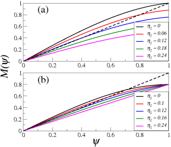
Figure 3: (Color online) Graph of the dynamical mapping $M(\psi)$ as a function of $\psi$ for $K=3$. (a) $\eta_{1}=0.1$ and different values of $\eta_{2}$; (b) $\eta_{2}=0.1$ and different values of $\eta_{1}$. Note that in both cases, as the noise intensity decreases the stable nonzero fixed point appears continuously. This is always the behavior for finite values of $K$.

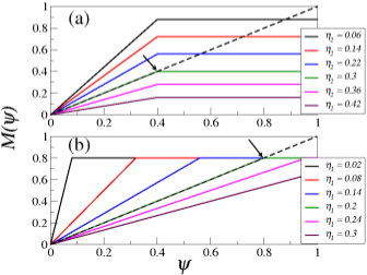
Figure 4: (Color online) Graph of the dynamical mapping $M(\psi)$ as a function of $\psi$ for $K\to\infty$. (a) $\eta_{1}=0.1$ and different values of $\eta_{2}$; (b) $\eta_{2}=0.1$ and different values of $\eta_{1}$. Note that in both cases, as the noise intensity decreases the stable nonzero fixed point appears discontinuously (indicated by the arrows). For infinite $K$, the phase transition is always discontinuous.

III.1.3 Sub-case 3: $\eta_{1}\neq 0$ and $\eta_{2}\neq 0$

When both types of noise, intrinsic and extrinsic, are present in the system, the phase transition is always continuous for any finite value of $K$. To illustrate this we present in Fig. 3(a) the graph of $M(\psi)$ for $\eta_{1}=0.1$ and different values of $\eta_{2}$. Note that $M(\psi)$ is a monotonically increasing convex function, and therefore the nonzero stable fixed point appears continuously as $\eta_{2}$ decreases. The same happens if we now fix the value of $\eta_{2}$ and vary the value of $\eta_{1}$, as it is shown in Fig. 3(b). This behavior is typical of a second order phase transition.

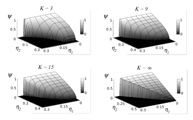
Figure 5: Phase transition in the majority voter model. Order parameter $\psi$ as a function of the extrinsic noise $\eta_{1}$ and the intrinsic noise $\eta_{2}$ for $K=3$, $K=9$, $K=15$ and $K\to\infty$. Note that for any finite value of $K$ the phase transition is always continuous except for the case $\eta_{1}=0$. Note also that the phase transition it is always discontinuous for $K\to\infty$.

Assuming $\psi\neq 0$ and using Eq. (12a), the fixed point equation $\psi=M(\psi)$ can be solved for $\psi$ obtaining

$$\psi=\pm\left\{\frac{1}{\beta_{3}^{3}(\eta_{1})}\left(\frac{1}{1-2\eta_{2}}-\beta_{1}^{3}(\eta_{1})\right)\right\}^{1/2}$$ (17)

For this equation to have real solutions the quantity inside the curly brackets must be positive. From Eq. (12c) it follows that $\beta_{3}^{3}(\eta_{1})\leq 0$ for any positive value of $\eta_{1}$. Therefore, Eq. (17) has real solutions only if

$$\frac{1}{1-2\eta_{2}}\leq\beta_{1}^{3}(\eta_{1}).$$

The values of $\eta_{1}$ and $\eta_{2}$ for which the equality holds in the above expression determine the critical line on the $\eta_{1}$-$\eta_{2}$ plane at which the phase transition occurs. Fig. 5 shows surface plots for the (positive) value of the stable fixed point $\psi$ as a function of $\eta_{1}$ and $\eta_{2}$ for $K=3$, $K=9$, $K=15$ and $K\to\infty$. Interestingly, for any finite value of $K$ the phase transition is always continuous except for the special case $\eta_{2}=0$. Therefore, for any finite $K$, even a small amount of intrinsic noise suffices to make the phase transition continuous.

III.2 Case 2: $K=\infty$

In Appendix A we show that for $K\to\infty$ the temporal evolution of the order parameter is still given by the dynamical mapping Eq. (11a), where now $M(\psi)$ is

$$M(\psi)=\left\{\begin{array}[]{rlr}-(1-2\eta_{2})&\mbox{ if }&\psi<-4\eta_{1}\\ &&\\ \frac{1-2\eta_{2}}{4\eta_{1}}\psi&\mbox{ if }&|\psi|\leq 4\eta_{1}\\ &&\\ 1-2\eta_{2}&\mbox{ if }&\psi>4\eta_{1}\end{array}\right.$$ (18)

Fig. 4(a) shows the behavior of $M(\psi)$ for $K\to\infty$, $\eta_{1}=0.1$ and different values of $\eta_{2}$, and Fig. 4(b) shows the same kind of plots but now keeping $\eta_{2}=0.1$ and varying the value of $\eta_{1}$. It can be seen from Fig. 4(a) that the phase transition is discontinuous. Indeed, as $\eta_{2}$ decreases below the critical value $\eta_{2}^{c}=0.3$, the non-zero stable fixed point appears discontinuously (see the point indicated with an arrow in the figure). An analogous behavior occurs in Fig. 4(b) when $\eta_{1}$ reaches the value $\eta_{1}^{c}=0.2$. Thus, in the limit $K\to\infty$ the phase transition is always discontinuous (see Fig. 5). In this sense, the discontinuity in the phase transition observed when only extrinsic noise is used can be considered as a singular limit, either $\eta_{2}\to 0$ or $K\to\infty$, of a phase transition that is otherwise continuous.

IV The vectorial network model

The second network model that we analyze, which we will call the Vectorial Network Model (VNM), is much closer to the self-propelled model than the voter model presented in the previous section. As we will see later, the VNM corresponds to a mean-field theory of the self-propelled model. It consists of a network with $N$ nodes (or elements) which, as in the self-propelled model, are the two dimensional vectors $\vec{v}_{1}=e^{i\theta_{1}},\dots,\vec{v}_{N}=e^{i\theta_{N}}$ (represented as complex numbers). All the vectors have the same magnitude $|\vec{v}_{n}|=1$ but their orientations $\theta_{1},\dots\theta_{N}$ in the plane can change. Each vector $\vec{v}_{n}$ is connected to a fixed set of $k_{n}$ other vectors, ${\mathcal{I}}_{n}=\{\vec{v}_{n_{1}},\vec{v}_{n_{2}},\dots,\vec{v}_{n_{k_{n}}}\}$, from which $\vec{v}_{n}$ will receive an input signal. We will call this set the inputs of $\vec{v}_{n}$, and consider again the homogeneous random topology in which all the elements have exactly $K$ inputs chosen randomly from anywhere in the system. The input signal $\vec{U}_{n}(t)$ received by $\vec{v}_{n}$ from its $K$ inputs is defined as

$$\vec{U}_{n}(t)=\frac{1}{K}\sum_{j=1}^{K}\vec{v}_{n_{j}}(t)$$ (19)

For the interaction between the network elements we consider from the beginning a dynamic rule that already incorporates both types of noise, intrinsic and extrinsic:

$$\theta_{n}(t+1)=\mbox{Angle}\left[\vec{U}_{n}(t)+\eta_{1}e^{i\xi_{n}(t)}\right]+\eta_{2}\zeta_{n}(t),$$ (20)

where $\xi_{n}(t)$ and $\zeta_{n}(t)$ are independent random variables uniformly distributed in the interval $[-\pi,\pi]$. The noise intensities $\eta_{1}$ and $\eta_{2}$, which take constant values between 0 and 1, are the amplitudes of the extrinsic (Grégoire-Chaté) and intrinsic (Vicsek) types of noise, respectively. Note that, while in the self-propelled model the particles can move and thus the vectors $\vec{v}_{n}$ represent particle velocities, in the VNM the particles do not move. Rather, they are fixed to the nodes of the network. For this reason, in the VNM the vectors $\vec{v}_{n}$ cannot be considered as velocities, but just as a given property of the particles (such as spin).

IV.1 Equivalence between the VNM and the self-propelled model

The main difference between the self-propelled model and the VNM is that in the former the motion of the particles can produce correlations in space and time that couple the global order with the local density, affecting the phase transition. Such coupling is not present in the VNM unless we choose very specific network topologies that change over time. However, here we are interested only on the effects that the two different types of noise have on the phase transition. The VNM is especially suited for this analysis precisely because of the absence of such complicated dynamical effects as the coupling between order and density.

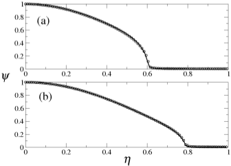
Figure 6: Phase transition for the VNM with intrinsic noise only (solid line) and the SPMIN with random mixing (symbols), both with $N=20000$. For the SPMIN the size of the box is $L=32$ and the radius $r$ of the interaction vicinity has been chosen so that the average number of interactions per particle coincides with the network connectivity $K$ in the VNM. The two panels correspond to (a) $K=5$ ($r\approx 0.285$)and (b) $K=20$ ($r\approx 0.571$). Note that the phase transition in this case is continuous and the same for both the VNM and the SPMIN with random mixing.

Nonetheless, it is important to note that the limit of large particle speeds of the self-propelled model is well described by the VNM. Indeed, if the speed of the particles in the self-propelled model is small, then particles that were within the same interaction vicinity at time $t$ will most likely remain within the same interaction vicinity at the next time step $t+\Delta t$. Therefore, for small particle speeds the spatial correlations between the particles are important. Contrary to this, in the opposite limit of large particle speeds, and because of the noise in the direction of motion of each particle (whether intrinsic or extrinsic), particles that at time $t$ were within the same vicinity will most likely not remain within that vicinity and end up interacting with different particles at the next time step $t+\Delta t$. Therefore, in the limit $v\to\infty$ of the self-propelled model spatial correlations are lost in only one time step. This is equivalent to randomly mixing the particles within the box at every time step, which is precisely the condition for the mean-field theory conveyed in the VNM to be exactly applicable.

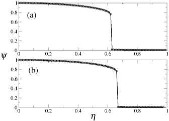
Figure 7: Phase transition for the VNM with extrinsic noise only (solid line) and the SPMEN with random mixing (symbols). The systems have the same parameters as in Fig. 6: $N=2\times 10^{4}$, $L=32$, $K=4$ ($r\approx 0.285$) in (a) and $K=20$ ($r\approx 0.571$) in (b). Note that the phase transition in this case is discontinuous and the same for both the VNM and the SPMEN with random mixing.

Fig. 6 shows the value of the order parameter $\psi$ as a function of the noise intensity $\eta$ for the VNM with intrinsic noise only (solid line), and for the SPMIN with random mixing (symbols) . Namely, instead of updating the positions of the particles in the SPMIN according to the kinematic rule given in Eq. (2c), we just randomly mixed all the particles within the box at every time step. We used equivalent systems with $N=20000$ particles and adjusted the other parameters of the SPMIN in such a way that the average number of interactions per particle $K$ was the same as for the vectorial network model [$K=5$ in Fig. 6(a) and $K=20$ in Fig. 6(b)]). Analogously, Fig. 7 shows equivalent results but for the VNM with extrinsic noise only (solid line) and the SPMEN with random mixing (symbols). As we can see from these figures, regardless of the type of noise both the self-propelled model with random mixing and the VNM give the same phase transition within numerical accuracy.

Although the above results do not constitute a proof, they do suggest that, in the limit of large particle speeds, the self-propelled model becomes equivalent to the VNM. It has been claimed that this equivalence is obtained only through a singular limit ChateComment . Though this might be the case, in our numerical simulations with different system sizes we always obtain results analogous to the ones displayed in Figs. 6 and 7, which do not seem to show such singular behavior.

IV.2 Mean-field theory of the VNM

Let us define the average vector $\vec{U}(t)$ as

$$\vec{U}(t)=\frac{1}{N}\sum_{n=1}^{N}\vec{v}_{n}(t).$$ (21)

In the context of the self-propelled model, $\vec{U}(t)$ is the average velocity of the entire system. Clearly, the instantaneous value of the order parameter $\psi(t)$ is related to this vector through $\psi(t)=\left|\vec{U}(t)\right|$. Let $(\psi(t),\theta(t))$ be the polar coordinates of $\vec{U}(t)$, and $P_{\vec{U}}(\psi,\theta;t)$ its probability distribution function (in polar coordinates). Note, then, that $\psi(t)$ is the first radial moment of $P_{\vec{U}}(\psi,\theta;t)$.

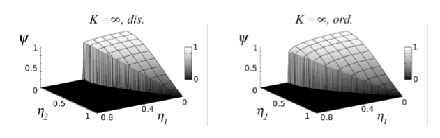
Figure 8: Phase transition in the VNM with $K\to\infty$. The left panel correspond to the phase transition obtained starting out the dynamics from a fully disordered condition ($\psi(0)\approx 0$), whereas for the panel on the right the dynamics were started from fully ordered initial conditions ($\psi(0)\approx 1$). In both cases the phase transition is discontinuous for any non-zero value of the extrinsic noise amplitude $\eta_{1}$. These plots were obtained by numerically finding the fixed points of $M(\psi)$ given in Eq. (25)

.

As in the voter model, we assume that the network elements $\vec{v}_{n}$ are statistically independent and equivalent. Therefore, Eq.(21) becomes the sum of $N$ independent and equally distributed random variables, and the problem of determining $\vec{U}(t)$ is then similar to that of finding the position of a 2D biased random walk. In Appendix B we present this mean-field calculation, and show that the temporal evolution of the Fourier transform of $P_{\vec{U}}(\psi,\theta;t)$ is given by the recurrence relation

$$\hat{P}_{\vec{U}}(\lambda,\gamma;t+1)=J_{0}(\lambda)+\sum_{m=-\infty}^{\infty}\frac{\sin(m\pi\eta_{2})}{2\pi^{2}\eta_{2}}J_{m}(\lambda)e^{im\gamma}$$ (22)

$$\times \int_{0}^{\infty}\frac{d\lambda^{\prime}}{\lambda^{\prime}}J_{0}(K\eta_{1}\lambda^{\prime})\int_{0}^{2\pi}d\gamma^{\prime}\left[\hat{P}_{\vec{U}}(\lambda^{\prime},\gamma^{\prime};t)\right]^{K}e^{-im\gamma^{\prime}},$$

where the $J_{m}(x)$’s are Bessel functions, and $\lambda$ and $\gamma$ are the Fourier conjugate variables to $\psi$ and $\theta$ respectively. In principle, this equation can be solved for any finite value of the network connectivity $K$. However, we were able to solve it only in the limit case $K\to\infty$. Therefore, we present first the analytic results for $K\to\infty$. In the next section we present numerical results for finite values of $K$.

IV.3 Case 1: $K\to\infty$

In the limit $K\to\infty$ the factor $\left[\hat{P}_{\vec{U}}(\lambda^{\prime},\gamma^{\prime};t)\right]^{K}$ appearing in the second integral of Eq. (22) can be replaced by a Dirac delta function radially centered at $K\psi(t)$. This leads to

$$\hat{P}_{\vec{U}}(\lambda,\gamma;t+1) = J_{0}(\lambda)+\sum_{m=-\infty}^{\infty}(-i)^{m}\frac{\sin(m\pi\eta_{2})}{\pi\eta_{2}}J_{m}(\lambda)$$ (23)

$$\times e^{im(\gamma-\alpha)}\int_{0}^{\infty}\frac{dx}{x}J_{0}(\eta x)J_{m}\left(\psi(t)x\right),$$

From this equation it follows that the order parameter $\psi(t)$, which is the first radial moment of $P_{\vec{U}}(\psi,\theta;t)$, obeys the dynamical mapping (see details in Appendix B)

$$\psi(t+1)=\frac{\sin(\pi\eta_{2})}{\pi\eta_{2}}\int_{0}^{\infty}J_{0}(\eta_{1}x)J_{1}\left(\psi(t)x\right)\frac{dx}{x}.$$ (24)

The integral on the right-hand side of the above equation is an instance of the Weber-Schafheitlin integrals A_and_S . After the evaluation of this integral, the dynamical mapping for the order parameter can be written as

$$\psi(t+1)=M\left(\psi(t)\right),$$ (25a)

where the mapping $$M(\psi)$$ is

$$M(\psi)=\left\{\begin{array}[]{lll}\frac{\sin(\pi\eta_{2})\psi(t)}{2\pi\eta_{1}\eta_{2}}{}_{2}F_{1}\left(\frac{1}{2},\frac{1}{2};2,\left[\frac{\psi}{\eta_{1}}\right]^{2}\right)&\mbox{ if }&\psi<\eta_{1}\\ &&\\ \frac{\sin(\pi\eta_{2})}{\pi\eta_{2}}{}_{2}F_{1}\left(\frac{1}{2},-\frac{1}{2};1,\left[\frac{\eta_{1}}{\psi}\right]^{2}\right)&\mbox{ if }&\psi>\eta_{1}\end{array}\right.$$ (25b)

and ${}_{2}F_{1}(a,b;c,d)$ are hypergeometric functions. The fixed points of $M(\psi)$ give the stationary value $\psi$ of the order parameter. In Ref. OurPRL we have shown that for $\eta_{2}=0$, the non-trivial fixed point of this mapping appears discontinuously as $\eta_{1}$ crosses the critical value $\eta_{1}\approx 0.672$ from above. On the other hand, for $\eta_{2}>0$ there is a global factor $\frac{\sin(\pi\eta_{2})}{\pi\eta_{2}}$ which does not change the discontinuous appearance of the non-trivial fixed point. Therefore, for any values of $\eta_{1}$ and $\eta_{2}$, the phase transition is discontinuous.

Fig. 8 shows surface plots of the stationary value $\psi$ as a function of $\eta_{1}$ and $\eta_{2}$ for two different cases: (i) when the dynamics of the VNM start out from disordered initial conditions [$\psi(0)\approx 0$ in Eq. (25a)], and (ii) when the dynamics start out from ordered initial conditions [$\psi(0)\approx 1$ in Eq. (25a)]. Let us denote as $\psi_{dis}$ and $\psi_{ord}$ the stationary values of the order parameter obtained in each of the two cases mentioned above, respectively. It is apparent from Fig. 8 that $\psi_{ord}$ and $\psi_{dis}$ are equal in a large region of the $\eta_{1}$-$\eta_{2}$ parameter space. However, there is also a region in which $\psi_{ord}$ and $\psi_{dis}$ are different. This latter region, where the system shows hysteresis, is shown in Fig. 9, in which the difference $\Delta\psi=\psi_{ord}-\psi_{dis}$ is plotted as a function of $\eta_{1}$ and $\eta_{2}$. The region for which $\Delta\psi\neq 0$ is a region of metastability where two stable fixed points exist, the trivial one $\psi_{dis}=0$ and the non-zero fixed point $\psi_{ord}$. It is clear from these results that the VNM with $K\to\infty$ exhibits a discontinuous phase transition for any non-zero value of the extrinsic noise $\eta_{1}$. On the other hand, for $\eta_{1}=0$, the amount of order in the system decreases as $\eta_{2}$ increases. However, there is no phase transition in this case since $\psi=0$ only when $\eta_{2}$ reaches its maximum value $\eta_{2}=1$. (In ferromagnetic systems, $\eta_{2}=1$ would correspond to infinite temperature.) In other words, for infinite connectivity and zero extrinsic noise, the order in the system can never be destroyed by the intrinsic noise, unless it reaches its maximum value. However, in the presence of both types of noise, extrinsic and intrinsic, the phase transition is always discontinuous.

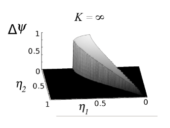
Figure 9: Difference $\Delta\psi=\psi_{ord}-\psi_{dis}$ between the two surface plots displayed on Fig. 8. The region for which $\Delta\psi\neq 0$ is the region of metastability where the system exhibits hysteresis. Note that this region crosses the entire square $[0,1]\times[0,1]$ in the $\eta_{1}$-$\eta_{2}$ plane from one side to the other.

IV.4 Case 2: $K$ finite

As it was mentioned before, we do not have an analytic solution of Eq. (22) for finite values of $K$. Nonetheless, numerical simulations show a phase transition that is continuous in one region of the $\eta_{1}$-$\eta_{2}$ parameter space, and discontinuous in another region. This is qualitatively different from the phase transition observed in the majority voter model, which was always continuous for any finite value of $K$ (except for $\eta_{2}=0$).

Fig. 10 shows $\psi$ as a function of $\eta_{1}$ and $\eta_{2}$ for different values of $K$. The results reported in this figure were obtained through numerical simulations of the VNM for systems with $N=20000$. The figures on the left correspond to disordered initial conditions ($\psi(0)\approx 0$), whereas those on the right correspond to ordered initial conditions ($\psi(0)\approx 1$). The difference $\Delta\psi=\psi_{ord}-\psi_{dis}$ as a function of $\eta_{1}$ and $\eta_{2}$ is plotted on Fig. 11. It is apparent from these figures that, except for the case $K=3$, there is a region of hysteresis where $\Delta\psi\neq 0$. This region grows as $K$ increases, but it does not seem to cross the square $[0,1]\times[0,1]$ of the $\eta_{1}$-$\eta_{2}$ parameter space from one side to the other (as it does for $K\to\infty$). This implies that the phase transition is discontinuous along the boundary of the region in which $\Delta\psi\neq 0$, but it is continuous along the boundary where $\psi\to 0^{+}$ and $\Delta\psi=0$.

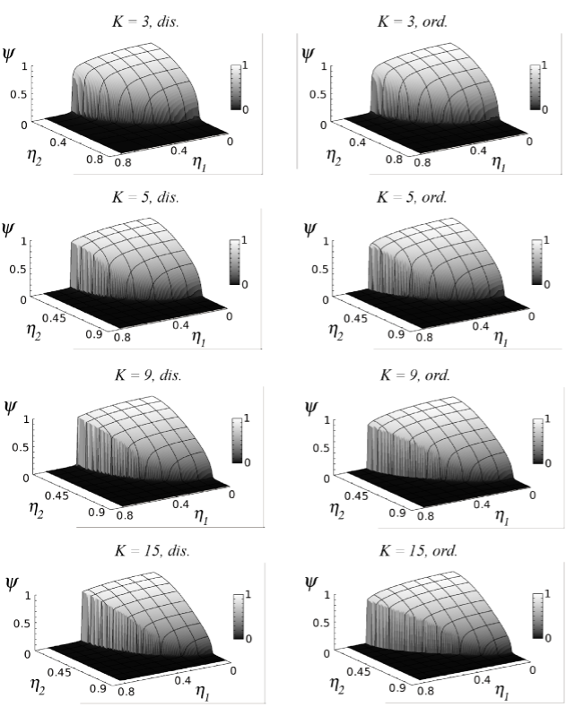
Figure 10: Surface plots show the order parameter $\psi$ as a function of the extrinsic and extrinsic noise amplitudes $\eta_{1}$ and $\eta_{2}$ respectively, for $K=3$, $K=5$, $K=9$ and $K=15$. The graphs were obtained through numerical simulation for systems with $K=2000$ elements. The panels on the left correspond to random initial conditions, whereas the panels on the right correspond to fully ordered initial conditions. Note that, except for the case $K=3$, there is a region of hysteresis where the phase transition is discontinuous.

It is worth emphasizing that for $\eta_{1}=0$, namely when there is no extrinsic noise, the VNM always undergoes a continuous phase transition from ordered to disordered states as the intensity of the intrinsic noise $\eta_{2}$ increases. This is consistent with the behavior originally reported by Vicsek et. al. for the SPMIN [see Fig. 1(a)]. On the other hand, for $\eta_{2}=0$, i.e. in the absence of intrinsic noise, the phase transition in the VNM is discontinuous as a function of the extrinsic noise amplitude $\eta_{1}$, which is consistent with the phase transition observed in the SPMEN [see Fig. 1(b)].

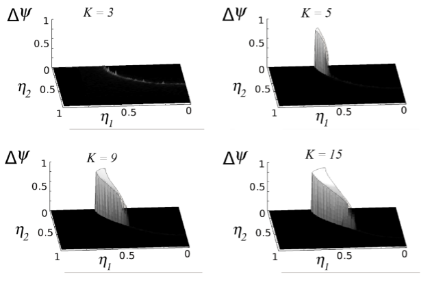
Figure 11: Difference $\Delta\psi=\psi_{ord}-\psi_{dis}$ between the surface plots displayed on Fig. 10. The region of metastability where $\Delta\psi\neq 0$ grows with $K$. However, for any finite value of $K$ this region does not cross the entire square $[0,1]\times[0,1]$ in the $\eta_{1}$-$\eta_{2}$ plane.

V What do we mean by “mean-field” theory?

In the computations of these two network models we have used the “mean field” assumption that all the spins are statistically independent and statistically equivalent, though we consider arbitrary values of $K$ (the number of particles that interact). This leads to phase transitions that can be continuous or discontinuous depending upon the values of $\eta_{1}$ and $\eta_{2}$. However, a frequent (and frequently equivalent) view of what constitutes a “mean field” theory entails the assumption that every particle interacts with all the other particles in the system. This second assumption is akin to the case $K\to\infty$, for which the phase transition is always discontinuous and, in general, of a different nature than the one obtained for finite $K$.

In our network models, the assumption of statistical independence is certainly true for the homogeneous random topology in which the $K$ inputs of each element are randomly chosen from anywhere in the system. In this case, the probability for two distinct elements $\vec{v}_{m}$ and $\vec{v}_{n}$ to have at least one of its $K$ inputs in common is of order $1/N$. In the thermodynamic limit $N\to\infty$ this probability is zero. Therefore, for large systems all the elements have different sets of inputs and are indeed statistically independent.

For other topologies, such as small-world, a large fraction of the network elements share inputs even in the thermodynamic limit. For this topology the assumption of statistical independence is no longer valid. However, the qualitative behavior of the phase transition obtained for the VNM on small-world networks, in which the short-range interactions induce spatial correlations between the network elements, is similar to the one observed for the homogeneous random topology described so far. Fig. 12 shows the phase transition in the VNM on small-world networks. To generate this figure we used the standard Watts-Strogatz small-world algorithm Watts3 ; Watts4 ; Strogatz , placing the elements on a 2D square lattice. Initially each element $\vec{v}_{n}$ has $K=5$ inputs, which are chosen as its four first-neighbors and the element $\vec{v}_{n}$ itself (i.e., we allow self-interactions). Then, with probability $p$ each input connection in the network is rewired to a randomly chosen element. Thus, if $p=0$ we have a regular square lattice, whereas if $p=1$ the topology becomes homogeneously random. This latter case is where our mean-field theory results are exactly applicable.

Fig. 12(a) corresponds to the case in which there is no intrinsic noise ($\eta_{2}=0$) and only the extrinsic noise is present, and Fig. 12(b) shows the opposite case where there is no extrinsic noise ($\eta_{1}=0$). The different curves in each figure correspond to different values of the rewiring probability $p$. Note that the nature of phase transition, i.e. whether continuous or discontinuous, does not change with the rewiring probability $p$. What changes is the critical value of the noise at which the phase transition occurs, but the continuity of the phase transition does not change with $p$. This is important because for small values of $p$ there are strong spatial correlations in the system generated by the first-neighbor interactions in the small-world network. However, even in the presence of such spatial correlations, the phase transition appears to be discontinuous for the extrinsic noise and continuous for the intrinsic noise. One advantage of the VNM is that the finite-size effects are much smaller than in the self-propelled model. Therefore, the continuous or discontinuous character of the phase transiion can be very well observed with $N=20000$ particles.

VI Summary and discussion

Although the self-propelled model proposed by Vicsek et. al. is one of the simplest models that we have to describe the emergence of collective order in groups of organisms, its analytic solution has remained elusive for more than a decade. Due to this lack of an analytical formalism to analyze the dynamical properties of the self-propelled model, it has not been possible to properly characterize some of its most basic features. In this work we have been particularly interested in how the way in which the noise is introduced in the system affects the nature of the phase transition. In the self-propelled model, numerical simulations indicate that the intrinsic noise originally proposed by Vicsek and his group seems to produce a continuous phase transition. In contrast, the extrinsic noise later introduced by Grégoire and Chaté generates a phase transition that is clearly discontinuous.

To determine the effect that each type of noise has on the phase transition, we have presented two network models that capture the main characteristics of the interactions in the self-propelled model and that can be handled analytically. These two network models, which we call the majority voter model and the vectorial network model, can be considered as the mean-field representation of the self-propelled model in 1 and 2 dimensions. In fact, we have shown numerically that the self-propelled model with random mixing, which is obtained in the limit of large particle speeds, is fully equivalent to the vectorial network model.

When the number of interactions per particle is finite, our numeric and analytic results for the two network models show that, in the absence of extrinsic noise, the phase transition driven by the intrinsic noise is continuous, in accordance with the results obtained for the original Vicsek model (SPMIN). In the opposite case, namely when there is no intrinsic noise and only the extrinsic noise is present, the phase transition is discontinuous, which is consistent with the behavior reported by Grégoire and Chaté for the SPMEN. The above results are true even for the small-world topology in which there exist strong spatial correlations induced by the first-neighbor connections.

For intermediate cases in which both types of noise are present, and for finite network connectivities, the situation is more complicated: The voter model exhibits a phase transition that is always continuous, whereas for the vectorial model there is a region in the noise-parameter space where the phase transition is continuous, and another region where it is discontinuous. In this later case, the region of discontinuity grows as the network connectivity increases. Interestingly, in the limit of infinite network connectivities and in the presence of both types of noise, the phase transition is always discontinuous in both the voter model and the vectorial model.

An interesting open question that follows from our work is to what extent can the stationary collective features of the network systems agree quantitatively with those of the corresponding swarming models. It has been suggested that the coupling between global order and local density could make the phase transition in the self-propelled model discontinuous regardless of the type of noise ChateComment . However, it is not clear how such coupling intervenes in the onset of collective order in the self-propelled model, nor how it can change the phase transition from continuous to discontinuous. To explore this idea, and more importantly, to determine whether or not the results obtained for the network models presented here can be applied to the self-propelled model, further analysis of the relation between the dynamics of a swarming system and the connectivity of its corresponding network representation is required.

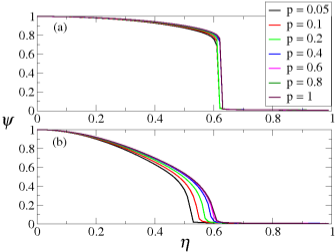
Figure 12: (Color online.) Phase transition in the VNM on small-world networks. (a) In the absence of intrinsic noise, the extrinsic noise produces a discontinuous phase transition regardless of the rewiring connectivity $p$. (b) The phase transition is continuous for all values of $p$ when only the intrinsic noise is present.

Appendix A Analytic results for the Majority Voter Model

In this appendix we present the analytic computation leading to Eqs. (11) and (18). Let us start by defining the quantities

$$\chi_{n}(t) = 4K\eta_{1}\xi_{n}(t),$$ (26a)

$$u_{n}(t) = \sum_{j=1}^{K}v_{n_{j}}(t),$$ (26b)

$$s_{n}(t) = u_{n}(t)+\chi_{n}(t).$$ (26c)

With these definitions, the dynamical interaction rule Eq. (10) can be rewritten in the equivalent form

$$v_{n}(t+1)=\left\{\begin{array}[]{rcc}\mbox{Sign}\left[s_{n}(t)\right]&\mbox{with prob.}&1-\eta_{2}\\ &&\\ -\mbox{Sign}\left[s_{n}(t)\right]&\mbox{with prob.}&\eta_{2}\end{array}\right.$$ (27)

Let $\phi_{n}(t)$ and $P_{n}^{+}(t)$ be the probabilities that $v_{n}(t)=1$ and $s_{n}(t)>0$, respectively. From Eq. (27) it is clear that $\phi_{n}(t)$ and $P_{n}^{+}(t)$ are related through

$$\phi_{n}(t)=(1-\eta_{2})P_{n}^{+}(t)+(1-P_{n}^{+}(t))\eta_{2}.$$ (28)

The first term on the right-hand side of the above equation accounts for the case in which $s_{n}(t)>0$ and the Sign function is evaluated. The second term takes into account the case in which $s_{n}(t)<0$ and the $-$Sign function is evaluated. In both of these cases $v_{n}(t+1)$ will be positive.

Now, we introduce the mean-field assumptions used in this computation:

• The probabilities $\phi_{n}(t)$ and $P_{n}^{+}(t)$ are the same for all the elements in the network. This assumption states that all the network elements are statistically equivalent. Thus, from now on we will drop off the subscript “$n$” in these quantities and use the notation $\phi_{n}(t)=\phi(t)$ and $P_{n}^{+}(t)=P^{+}(t)$.

• That the network elements $v_{n}$ are statistically independent implies that the sum $u_{n}(t)$ defined in Eq. (26b) can be considered as the sum of $K$ independent and identically distributed random variables.

Note that the order parameter $\psi(t)=\langle v_{n}(t)\rangle$ can be expressed in terms the probability $\phi(t)$ as

$$\psi(t)=\langle v_{n}(t)\rangle=(1)\phi(t)+(-1)(1-\phi(t))=2\phi(t)-1,$$

from which we obtain

$$\phi(t)=\frac{1+\psi(t)}{2}.$$ (29)

Eq.(28) can then be written in terms of the order parameter $\psi(t)$ as

$$\psi(t+1)=2(1-2\eta_{2})P^{+}(t)+2\eta_{2}-1.$$ (30)

The next step in this calculation consists in expressing $P^{+}(t)$ as a function of $\phi(t)$, or equivalently, as a function of $\psi(t)$. To this end, let $P_{v}(x,t)$, $P_{u}(x,t)$, $P_{s}(x,t)$, and $P_{\chi}(x)$ be the probability density functions of the random variables $v_{n}(t)$, $u_{n}(t)$, $s_{n}(t)$ and $\chi_{n}(t)$, respectively. (Note that $P_{\chi}(x)$, the probability density function of the noise, is independent of time.) From Eq. (26c) it follows that

$$P_{s}(x,t)=[P_{u}*P_{\chi}](x,t),$$ (31)

where “$*$” denotes a convolution. Analogously, since $u_{n}(t)$ is the sum of the $K$ independent random variables $v_{n_{1}}(t),\dots,v_{n_{K}}(t)$, all equally distributed with the PDF $P_{v}(x,t)$, then $P_{u}(x,t)$ is the $K$-fold convolution of $P_{v}(x,t)$ with itself, and therefore, $P_{s}(x,t)$ becomes

$$P_{s}(x,t)=[\underbrace{P_{v}*\cdots*P_{v}}_{K\ times}*P_{\chi}](x,t).$$ (32)

It is convenient to transform the above equation to Fourier space (in the variable $x$). Denoting as $\hat{P}_{v}(\lambda,t)$, $\hat{P}_{u}(\lambda,t)$, $\hat{P}_{s}(\lambda,t)$ and $\hat{P}_{\chi}(\lambda)$ the Fourier transforms of the corresponding PDF’s, we obtain

$$\hat{P}_{s}(\lambda,t)=\left[\hat{P}_{v}(\lambda,t)\right]^{K}\hat{P}_{\chi}(\lambda,t).$$ (33)

We have now to consider two cases separately, the case for which $K<\infty$, and the case $K\to\infty$.

A.1 Case 1: $K<\infty$

By definition of $\phi(t)$, we have that

$$P_{v}(x,t)=\phi(t)\delta(x-1)+(1-\phi(t))\delta(x+1),$$

where $\delta(x)$ is the Dirac delta function. Therefore ,

$$\hat{P}_{v}(\lambda,t)=\phi(t)e^{-i\lambda}+(1-\phi(t))e^{i\lambda}.$$

The above equation can be written in terms of $\psi(t)$ by using the relationship given in Eq. (29), which gives

$$\hat{P}_{v}(\lambda,t)=\cos\lambda-i\psi(t)\sin\lambda.$$ (34)

On the other hand, $\chi_{n}(t)$ is a random variable uniformly distributed in the interval $[-4K\eta_{1},4K\eta_{1}]$, from which it follows that

$$\hat{P}_{\chi}(\lambda)=\frac{1}{4K\eta_{1}\lambda}\sin{4K\eta_{1}\lambda}.$$ (35)

Substituting into Eq. (33) the results given in Eqs. (34) and (35) we obtain

$$\hat{P}_{s}(\lambda,t) = \left[\cos\lambda-i\psi(t)\sin\lambda\right]^{K}\frac{\sin(4K\eta_{1}\lambda)}{4K\eta_{1}}$$ (36)

$$= \sum_{m=0}^{K}(-i)^{m}\binom{K}{m}[\cos\lambda]^{K-m}[\psi(t)\sin\lambda]^{m}$$

$$\times\frac{\sin(4K\eta_{1}\lambda)}{4K\eta_{1}\lambda}.$$

Since $P^{+}(t)$ is the probability that $s_{n}(t)>0$, then

$$P^{+}(t)=\int_{0}^{\infty}P_{s}(x,t)dx.$$

Therefore, taking the inverse Fourier transform of Eq. (36) and integrating the result from 0 to $\infty$ we obtain

$$P^{+}(t)=\frac{1}{2}\sum_{m=0}^{K}\beta_{m}^{K}(\eta_{1})[\psi(t)]^{m},$$ (37)

where the coefficients $\beta_{m}^{K}(\eta_{1})$ are given by

$$\beta_{m}^{K}(\eta_{1}) = \binom{K}{m}\frac{(-i)^{m}}{\pi 4K\eta_{1}}\int_{0}^{\infty}\int_{-\infty}^{\infty}[\cos\lambda]^{K-m}[\sin\lambda]^{m}$$ (38)

$$\times\frac{\sin(4K\eta_{1}\lambda)}{\lambda}e^{i\lambda x}d\lambda dx.$$

Although it is not obvious from the above expression, it happens that $\beta_{0}^{K}(\eta_{1})=1$. To show that this is indeed the case, let us define the function $\hat{G}(\lambda)$ as

$$\hat{G}(\lambda)=[\cos\lambda]^{K}\frac{\sin(4K\eta_{1}\lambda)}{4K\eta_{1}\lambda}.$$

Note that $\hat{G}(\lambda)$ is a symmetric function and that $\hat{G}(0)=1$. With this definition, the coefficient $\beta_{0}^{K}(\eta_{1})$ can be written as

$$\beta_{0}^{K}(\eta_{1}) = 2\int_{0}^{\infty}\frac{1}{2\pi}\int_{-\infty}^{\infty}\hat{G}(\lambda)e^{i\lambda x}d\lambda dx$$

$$= 2\int_{0}^{\infty}G(x)dx,$$

where $G(x)$ is the inverse Fourier transform of $\hat{G}(\lambda)$. Since $\hat{G}(\lambda)$ is symmetric, then $G(x)$ is also symmetric and therefore $\int_{-\infty}^{\infty}G(x)dx=2\int_{0}^{\infty}G(x)dx$. Additionally, since $\hat{G}(0)=1$ then $\int_{-\infty}^{\infty}G(x)dx=1$, from which it follows that $\beta_{0}^{K}(\eta_{1})=1$.

For $m\geq 1$ we can exchange the order of integration in Eq. (38) by multiplying the integrand by $e^{-\epsilon x}$. After performing the integral over $x$ and then taking the limit $\epsilon\to 0$ we obtain

$$\beta_{m}^{K}(\eta_{1}) = \binom{K}{m}\frac{(-i)^{m-1}}{\pi 4K\eta_{1}}$$ (39)

$$\times \int_{-\infty}^{\infty}[\cos\lambda]^{K-m}[\sin\lambda]^{m}\frac{\sin(4K\eta_{1}\lambda)}{\lambda^{2}}d\lambda.$$

Using the fact that $\beta_{0}^{K}(\eta_{1})=1$, Eq. (37) can be written as

$$P^{+}(t)=\frac{1}{2}\left(1+\sum_{m=1}^{K}\beta_{m}^{K}(\eta_{1})[\psi(t)]^{m}\right).$$

Finally, substituting the above result into Eq. (30) we obtain

$$\psi(t+1)=(1-2\eta_{2})\sum_{m=1}^{K}\beta_{m}^{K}(\eta_{1})[\psi(t)]^{m}.$$ (40)

A.2 Case 2: $K\to\infty$

By definition [see Eq. (26b)] $u_{n}(t)$ is the sum of $K$ independent and identically distributed variables, each with average $\psi(t)$ and variance $1-[\psi(t)]^{2}$. Therefore, for very large values of $K$ the Central Limit Theorem allows us to approximate $P_{u}(x,t)$ by a Gaussian with average $K\psi(t)$ and variance $\sigma^{2}=K(1-[\psi(t)]^{2})$

$$P_{u}(x,t)\approx\frac{\exp\left(-\frac{(x-K\psi(t))^{2}}{2K(1-[\psi(t)]^{2})}\right)}{\sqrt{2\pi K(1-[\psi(t)]^{2})}}.$$

With this approximation, Eq. (31) becomes

$$P_{s}(x,t) = \frac{1}{8K\eta_{1}\sqrt{2\pi K(1-[\psi(t)]^{2})}}$$

$$\times \int_{-4K\eta_{1}}^{4K\eta_{1}}\exp\left(-\frac{(x-y-K\psi(t))^{2}}{2K(1-[\psi(t)]^{2})}\right)dy,$$

where we have used the fact that $P_{\chi}(x)$ is a constant normalized function defined in the interval $x\in[-4K\eta_{1},4K\eta_{1}]$. From the above expression we can obtain $P^{+}(t)$ by integrating $P_{s}(x,t)$ from 0 to $\infty$:

$$P^{+}(t) = \frac{1}{8K\eta_{1}\sqrt{2\pi K(1-[\psi(t)]^{2})}}$$

$$\times \int_{0}^{\infty}\int_{-4K\eta_{1}}^{4K\eta_{1}}\exp\left(-\frac{(x-y-K\psi(t))^{2}}{2K(1-[\psi(t)]^{2})}\right)dydx.$$

Performing the change of variable $x=Kx^{\prime}$, $y=Ky^{\prime}$, the above expression transforms into

$$P^{+}(t) = \frac{1}{8\eta_{1}\sqrt{\frac{2\pi}{K}(1-[\psi(t)]^{2})}}$$

$$\times \int_{0}^{\infty}\int_{-4\eta_{1}}^{4\eta_{1}}\exp\left(-\frac{(x^{\prime}-y^{\prime}-\psi(t))^{2}}{\frac{2}{K}(1-[\psi(t)]^{2})}\right)dy^{\prime}dx^{\prime}.$$

In the limit $K\to\infty$ we have

$$\lim_{K\to\infty}\frac{\exp\left(-\frac{(x^{\prime}-y^{\prime}-\psi(t))^{2}}{\frac{2}{K}(1-[\psi(t)]^{2})}\right)}{\sqrt{\frac{2\pi}{K}(1-[\psi(t)]^{2})}}=\delta\left(x^{\prime}-y^{\prime}-\psi(t)\right),$$

where $\delta(\cdot)$ is the Dirac delta function. From the last two equations above it follows that, in the limit $K\to\infty$, the probability $P^{+}(t)$ acquires the simpler form

$$P^{+}(t)=\frac{1}{8\eta_{1}}\int_{0}^{\infty}\int_{-4\eta_{1}}^{4\eta_{1}}\delta\left(x^{\prime}-y^{\prime}-\psi(t)\right)dx^{\prime}dy^{\prime}.$$

After performing the integrals in the above expression we obtain

$$P^{+}(t)=\left\{\begin{array}[]{llr}0&\mbox{ if }&\psi(t)<-4\eta_{1}\\ &&\\ \frac{1}{8\eta_{1}}(\psi(t)+4\eta_{2})&\mbox{ if }&|\psi(t)|\leq 4\eta_{1}\\ &&\\ 1&\mbox{ if }&\psi(t)>4\eta_{1}\end{array}\right.$$

This last result combined with Eq. (30) give Eq. (18) of the main text.

Appendix B Analytic computation of the phase transition for the Vectorial network model

The dynamics of the Vectorial network model (VNM) are given by the interaction rule

$$\theta_{m}(t+1)=\mbox{Angle}\left[\sum_{j=1}^{K}\vec{v}_{m_{j}}(t)+K\eta_{1}e^{i\xi_{m}(t)}\right]+\eta_{2}\zeta_{m}(t),$$ (41)

where $\{\vec{v}_{m_{j}}\}_{j=1}^{K}$ are the $K$ inputs of $\vec{v}_{m}$, and $\xi_{m}(t)$ and $\zeta_{m}(t)$ are independent random variables uniformly distributed in the interval $[-\pi,\pi]$ and $0\leq\eta_{1},\eta_{2}\leq 1$. Let us define the extrinsic noise vector $\vec{n}_{e}$ and the intrinsic noise $n_{i}$ as

$$\vec{n}_{e} = K\eta_{1}e^{i\xi(t)},$$

$$n_{i} = \eta_{2}\zeta.$$

We will denote as $P_{\vec{n}_{e}}(r,\xi)$ the PDF (in polar coordinates) of the extrinsic noise $\vec{n}_{e}$ and as $P_{n_{i}}(\zeta)$ the PDF of the intrinsic noise $n_{i}$. As for the majority voter model, it is convenient to define the quantities

$$\vec{u}_{m}(t) = \sum_{j=1}^{K}\vec{v}_{m_{j}}(t),$$ (42)

$$\vec{s}_{m}(t) = \vec{u}_{m}(t)+\vec{n}_{e}(t).$$ (43)

Let $(v_{m},\theta_{m})$, $(u_{m},\beta_{m})$ and $(s_{m},\theta^{\prime}_{m})$ be the polar coordinates of the vectors $\vec{v}_{m}(t)$, $\vec{u}_{m}(t)$, and $\vec{s}_{m}(t)$, respectively. We will denote as $P_{\vec{v}_{m}}(v_{m},\theta_{m};t)$, $P_{\vec{u_{m}}}(u_{m},\beta_{m};t)$, and $P_{\vec{s}_{m}}(s_{m},\theta^{\prime}_{m};t)$ the PDF’s of these three vectors, respectively. In Table 1 we summarize the relevant quantities appearing in this calculation.

Scalar	Amplitude	PDF	Fourier Transform
$n_{i}=\eta_{2}\zeta(t)$	$\eta_{2}$	$P_{n_{i}}(\zeta)$	$\hat{p}_{m}$
Vector	Polar Coor.	PDF	Fourier Transform
$\vec{n}_{e}(t)=K\eta_{1}e^{i\xi(t)}$	$(r,\xi)$	$P_{\vec{n}_{e}}(r,\xi)$	$\hat{P}_{\vec{n}_{e}}(\lambda,\gamma)$
$\vec{v}_{m}(t)=e^{i\theta_{m}(t)}$	$(v,\theta)$	$P_{\vec{v}}(v,\theta;t)$	$\hat{P}_{\vec{v}}(\lambda,\gamma;t)$
$\vec{u}_{m}(t)=\sum_{j=1}^{K}\vec{v}_{m_{j}}(t)$	$(u,\beta)$	$P_{\vec{u}}(u,\beta;t)$	$\hat{P}_{\vec{u}}(\lambda,\gamma;t)$
$\vec{s}_{m}(t)=\vec{u}_{m}(t)+\vec{\eta}(t)$	$(s,\theta^{\prime})$	$P_{\vec{s}}(s,\theta^{\prime};t)$	$\hat{P}_{\vec{s}}(\lambda,\gamma;t)$

Table 1: Notation guide for the different quantities involved in the calculation of the phase transition of the VNM. We have omitted the subscript $m$ in the PDF’s since we assume that all the network elements $\vec{v}_{m}$ are statistically equivalent.

Note that neither $P_{\vec{n}_{e}}(r,\xi)$ nor $P_{n_{i}}(\zeta)$ depend on time or on the subscript $m$ of $\vec{v}_{m}$, whereas the PDF’s of $\vec{v}_{m}(t)$, $\vec{u}_{m}(t)$, and $\vec{s}_{m}(t)$ depend on both time and the subscript $m$. However, in a mean-field approximation, we can assume that all the vectors $\vec{v}_{m}$ are statistically equivalent and statistically independent. In this case, the functions $P_{\vec{v}_{m}}(v_{m},\theta_{m};t)$, $P_{\vec{u_{m}}}(u_{m},\beta_{m};t)$, and $P_{\vec{s}_{m}}(s_{m},\theta^{\prime}_{m};t)$ are site independent, (i.e., the same for all the vectors in the network) and the subscript $m$ can be omitted. From now on we will assume that the conditions for the validity of the mean-field approximation (statistical equivalence and independence) apply.

B.1 The order parameter

To measure the amount of order in the system, we define the instantaneous order parameter $\psi(t)$ as

$$\psi(t)=\left|\frac{1}{N}\sum_{m=1}^{\infty}\vec{v}_{m}(t)\right|=\left|\left\langle\vec{v}(t)\right\rangle\right|,$$ (44)

where we have defined $\left\langle\vec{v}(t)\right\rangle=\frac{1}{N}\sum_{m=1}^{\infty}\vec{v}_{m}(t)$. Under the mean-field assumption, all the vectors $\vec{v}_{m}$ are equally distributed with the common probability distribution $P_{\vec{v}}(v,\theta;t)$. Then $\left\langle\vec{v}(t)\right\rangle$ can be computed as follows.

Let $\hat{P}_{\vec{v}}(\lambda,\gamma;t)$ be the Fourier transform (in polar coordinates) of $P_{\vec{v}}(v,\theta;t)$. The variables $\lambda$ and $\gamma$ are the Fourier conjugates of the variables $v$ and $\theta$, respectively. A cumulant expansion of $\hat{P}_{\vec{v}}(\lambda,\gamma;t)$ up to the first order gives

$$\hat{P}_{\vec{v}}(\lambda,\gamma;t)\approx 1-i\langle\vec{v}(t)\rangle\cdot\vec{\lambda}+\cdots,$$ (45)

where $\vec{\lambda}$ is the vector in Fourier space whose polar coordinates are $(\lambda,\gamma)$. Denoting as $\alpha$ the angle between $\langle\vec{v}(t)\rangle$ and $\vec{\lambda}$, and using the fact that $\psi(t)=\left|\langle\vec{v}(t)\rangle\right|$, Eq. (45) can be written as

$$\hat{P}_{\vec{v}}(\lambda,\gamma;t)\approx 1-i\psi(t)\lambda\cos\alpha+\cdots.$$ (46)

Thus, a first order cumulant expansion of $\hat{P}_{\vec{v}}(\lambda,\gamma;t)$ directly gives us the order parameter $\psi(t)$. The objective of the calculation is to find a recurrence relation in time for $\hat{P}_{\vec{v}}(\lambda,\gamma;t)$ based on Eq. (41). From this recurrence relation we will obtain the dynamical mapping that determines the temporal evolution of $\psi(t)$.

B.2 Recurrence relation for $\hat{P}_{\vec{v}}(\lambda,\gamma;t)$

Note first that, since $|\vec{v}_{m}|=1$ for all $m$, then $P_{\vec{v}}(v,\theta;t)$ can be written as

$$P_{\vec{v}}(v,\theta;t)=\frac{\delta(v-1)}{v}P_{\theta}(\theta;t),$$ (47)

where $P_{\theta}(\theta;t)$ is the PDF of the angle $\theta(t)$ of $\vec{v}(t)$. From Eq. (41) it follows that $P_{\theta}(\theta;t)$, $P_{\vec{s}}(s,\theta;t)$ and $P_{n_{i}}(\zeta)$ are related through

$$P_{\theta}(\theta;t+1)=\int_{-\pi}^{\pi}\left[\int_{0}^{\infty}sP_{\vec{s}}(s,\theta-\zeta;t)ds\right]P_{n_{i}}(\zeta)d\zeta.$$ (48)

Since $\vec{s}(t)=\sum_{j=1}^{K}\vec{v}_{m_{j}}(t)+\vec{n}_{e}(t)$, and each of the vectors $\vec{v}_{m_{j}}(t)$ is distributed with the PDF $P_{\vec{v}}(v,\theta;t)$, it is clear that $P_{\vec{s}}(s,\theta;t)$ depends on $P_{\theta}(\theta;t)$. Therefore, Eq. (48) is a recurrence relation in time for $P_{\theta}(\theta;t)$. This recurrent relation is best solved in Fourier space. Denoting as $\hat{P}_{\vec{s}}(\lambda,\gamma;t)$ the Fourier transform of $P_{\vec{s}}(s,\theta;t)$, the above equation can be written as

$$P_{\theta}(\theta;t+1) = \frac{1}{(2\pi)^{2}}\int_{-\pi}^{\pi}d\zeta\int_{0}^{\infty}sds\int_{0}^{\infty}\lambda d\lambda\int_{0}^{2\pi}d\gamma$$ (49)

$$\times \hat{P}_{\vec{s}}(\lambda,\gamma-\zeta;t)P_{n_{i}}(\zeta)e^{is\lambda\cos(\gamma-\theta)}.$$

Since $P_{\theta}(\theta;t)$, $\hat{P}_{\vec{s}}(\lambda,\gamma;t)$ and $P_{n_{i}}(\zeta)$ are periodic functions of their angular arguments ($\theta$, $\gamma$ and $\zeta$ respectively), we can expand these functions in Fourier series as

$$P_{\theta}(\theta;t) = \sum_{m=-\infty}^{\infty}\phi_{m}(t)e^{im\theta},$$ (50)

$$\hat{P}_{\vec{s}}(\lambda,\gamma-\zeta;t) = \sum_{m=-\infty}^{\infty}\chi_{m}(\lambda;t)e^{im(\gamma-\zeta)},$$ (51)

$$P_{n_{i}}(\zeta) = \sum_{m=-\infty}^{\infty}\hat{p}_{m}e^{-im\zeta},$$ (52)

where $\phi_{m}(t)$, $\chi_{m}(\lambda;t)$ and $\hat{p}_{m}$ are given by

$$\phi_{m}(t) = \frac{1}{2\pi}\int_{-\pi}^{\pi}P_{\theta}(\theta;t)e^{-im\theta}d\theta,$$ (53)

$$\chi_{m}(\lambda;t) = \frac{1}{2\pi}\int_{-\pi}^{\pi}\hat{P}_{\vec{s}}(\lambda,\gamma;t)e^{-im\gamma}d\gamma,$$ (54)

$$\hat{p}_{m} = \frac{1}{2\pi}\int_{-\pi}^{\pi}P_{n_{i}}(\zeta)e^{-im\zeta}d\zeta.$$ (55)

Substituting Eqs.(50) and (51) into Eq. (49), carrying out the integration over $\zeta$ and taking into account Eq.(55) we obtain

$$\sum_{m=-\infty}^{\infty}\phi_{m}(t+1)e^{im\theta}$$

$$= \sum_{m=-\infty}^{\infty}(i)^{m}\hat{p}_{m}\int_{0}^{\infty}sds\int_{0}^{\infty}\lambda d\lambda\chi_{m}(\lambda;t)J_{m}(s\lambda)e^{im\theta},$$

where we have used the integral representation of the Bessel function $J_{m}(x)=\frac{(-i)^{m}}{2\pi}\int_{0}^{2\pi}e^{i(mz+x\cos z)}dz$. It follows from the last expression that

$$\phi_{m}(t+1)=i^{m}\hat{p}_{m}\int_{0}^{\infty}sds\int_{0}^{\infty}\lambda d\lambda\chi_{m}(\lambda;t)J_{m}(s\lambda).$$ (56)

Exchanging the order of integration in the last expression, and using the identity

$$\int_{0}^{\infty}sJ_{m}(\lambda s)ds=\frac{\delta(\lambda)}{\lambda}\delta_{m,0}+\frac{m}{\lambda^{2}},$$

where $\delta(\lambda)$ and $\delta_{m,0}$ are the Dirac and Kronecker delta functions, respectively, Eq. (56) becomes

$$\phi_{m}(t+1)=(i)^{m}\hat{p}_{m}\left(\delta_{m,0}\chi_{m}(0;t)+m\int_{0}^{\infty}\chi_{m}(\lambda;t)\frac{d\lambda}{\lambda}\right).$$ (57)

Note that Eq. (57) is a consequence of the recurrence relation given in Eq. (48), which in turn follows directly from the dynamic interaction rule Eq. (41). Now we have to project the probability distribution function $P_{\vec{s}}(s,\theta;t)$ onto the unit circle by forcing the vector $\vec{s}(t)$ to have unit length at time $t+1$, and thus becoming $\vec{v}(t)$. To do so, we take the Fourier transform of $P_{\vec{v}}(v,\theta;t)$ given in Eq. (47), which when evaluated at time $t+1$ gives

$$\hat{P}_{\vec{v}}(\lambda,\gamma;t+1)=\int_{0}^{2\pi}P_{\theta}(\theta;t+1)e^{-i\lambda\cos(\theta-\gamma)}d\theta.$$ (58)

Substituting into the above equation the form of $P_{\theta}(\theta;t)$ given in Eq. (50) (evaluated at $t+1$), we obtain

$$\hat{P}_{\vec{v}}(\lambda,\gamma;t+1)=2\pi\sum_{m=-\infty}^{\infty}(-i)^{m}\phi_{m}(t+1)J_{m}(\lambda)e^{im\gamma},$$ (59)

where we have used the integral representation of the Bessel function $J_{m}(\lambda)=\frac{(i)^{m}}{2\pi}\int_{0}^{2\pi}e^{i(mz-\lambda\cos z)}dz$. Now we use the value of $\phi_{m}(t+1)$ given in Eq. (57), which leads to

$$\hat{P}_{\vec{v}}(\lambda,\gamma;t+1) = 2\pi\hat{p}_{0}J_{0}(\lambda)+\sum_{m=-\infty}^{\infty}2\pi m\hat{p}_{m}J_{m}(\lambda)e^{im\lambda}$$ (60)

$$\times \int_{0}^{\infty}\chi_{m}(\lambda^{\prime};t)\frac{d\lambda^{\prime}}{\lambda^{\prime}}.$$

To complete the projection of $\hat{P}_{\vec{v}}(\lambda,\gamma;t)$ onto the unit circle in a closed form, it only remains to find $\chi_{m}(t)$ as a function of $\hat{P}_{\vec{v}}(\lambda,\gamma;t)$. Since $s(t)=\sum_{j=1}^{K}\vec{v}_{m_{j}}(t)+\vec{n}_{e}(t)$, and we are assuming that all the $\vec{v}_{j}$ are statistically independent, then

$$\hat{P}_{\vec{s}}(\lambda,\gamma;t)=\left[\hat{P}_{\vec{v}}(\lambda,\gamma;t)\right]^{K}\hat{P}_{\vec{n}_{e}}(\lambda,\gamma),$$ (61)

where $\hat{P}_{\vec{n}_{e}}(\lambda,\gamma)$ is the Fourier transform of the PDF of the noise vector $\vec{n}_{e}=K\eta_{1}e^{i\xi}$. Since $\xi$ is uniformly distributed in the interval $[0,2\pi]$, it follows that $\hat{P}_{\vec{n}_{e}}(\lambda,\gamma)=J_{0}(K\eta\lambda)$. Therefore, we obtain

$$\hat{P}_{\vec{s}}(\lambda,\gamma;t)=\left[\hat{P}_{\vec{v}}(\lambda,\gamma;t)\right]^{K}J_{0}(K\eta\lambda).$$ (62)

Substituting the above expression into Eq. (54) we obtain

$$\chi_{m}(\lambda;t)=\frac{1}{2\pi}J_{0}(K\eta\lambda)\int_{0}^{2\pi}\left[\hat{P}_{\vec{v}}(\lambda,\gamma;t)\right]^{K}e^{-im\gamma}d\gamma.$$ (63)

Finally, combining this result with Eq. (60), we obtain the desired recurrence relation for $\hat{P}_{\vec{v}}(\lambda,\gamma;t)$:

$$\hat{P}_{\vec{v}}(\lambda,\gamma;t+1)=2\pi\hat{p}_{0}J_{0}(\lambda)+\sum_{m=-\infty}^{\infty}m\hat{p}_{m}J_{m}(\lambda)e^{im\gamma}$$ (64)

$$\times \int_{0}^{\infty}\frac{d\lambda^{\prime}}{\lambda^{\prime}}J_{0}(K\eta\lambda^{\prime})\int_{0}^{2\pi}d\gamma^{\prime}\left[\hat{P}_{\vec{v}}(\lambda^{\prime},\gamma^{\prime};t)\right]^{K}e^{-im\gamma^{\prime}}.$$

B.3 Dynamical mapping for $K\to\infty$

Eq. (64) is a complicated recurrence relation the exact solution to which is way out of our hands. However, for large values of $K$, namely, for a large number of interactions per particle, we can use the Central Limit Theorem to approximate $\left[\hat{P}_{\vec{v}}(\lambda,\gamma;t)\right]^{K}$ as

$$\left[\hat{P}_{\vec{v}}(\lambda,\gamma;t)\right]^{K}\approx\exp\left\{-iK\langle\vec{v}(t)\rangle\cdot\vec{\lambda}-\frac{K}{2}\vec{\lambda}\cdot{\mathbf{C}}(t)\cdot\vec{\lambda}\right\},$$

where $\langle\vec{v}(t)\rangle$ and ${\mathbf{C}}(t)$ are the first moment and covariance matrix of $P_{\vec{v}}(v,\theta;t)$, respectively, and $\vec{\lambda}$ is the vector in Fourier space with polar coordinates $(\lambda,\gamma)$. With this approximation, Eq. (64) becomes

$$\hat{P}_{\vec{v}}(\lambda,\gamma;t+1)=2\pi\hat{p}_{0}J_{0}(\lambda)+\sum_{m=-\infty}^{\infty}m\hat{p}_{m}J_{m}(\lambda)e^{im\gamma}$$

$$\times \int_{0}^{\infty}\frac{d\lambda^{\prime}}{\lambda^{\prime}}J_{0}(K\eta\lambda^{\prime})\int_{0}^{2\pi}d\gamma^{\prime}e^{-iK\langle\vec{v}(t)\rangle\cdot\vec{\lambda^{\prime}}-\frac{K}{2}\vec{\lambda^{\prime}}\cdot{\mathbf{C}}(t)\cdot\vec{\lambda^{\prime}}}e^{-im\gamma^{\prime}}.$$

Making the change of variable $\vec{x}=K\vec{\lambda^{\prime}}$ in the above expression, we obtain

$$\hat{P}_{\vec{v}}(\lambda,\gamma;t+1)=2\pi\hat{p}_{0}J_{0}(\lambda)+\sum_{m=-\infty}^{\infty}m\hat{p}_{m}J_{m}(\lambda)e^{im\gamma}$$

$$\times \int_{0}^{\infty}\frac{dx}{x}J_{0}(\eta x)\int_{0}^{2\pi}d\gamma^{\prime}e^{-i\langle\vec{v}(t)\rangle\cdot\vec{x}-\frac{1}{2K}\vec{x}\cdot{\mathbf{C}}(t)\cdot\vec{x}}e^{-im\gamma^{\prime}}.$$

We can go a step further in the large-$K$ approximation and neglect the term $\frac{1}{2K}\vec{x}\cdot{\mathbf{C}}(t)\cdot\vec{x}$ appearing in the exponent inside the integral of the last expression, which gives

$$\hat{P}_{\vec{v}}(\lambda,\gamma;t + 1)=2\pi\hat{p}_{0}J_{0}(\lambda)+\sum_{m=-\infty}^{\infty}m\hat{p}_{m}J_{m}(\lambda)e^{im\gamma}$$ (65)

$$\times \int_{0}^{\infty}\frac{dx}{x}J_{0}(\eta x)\int_{0}^{2\pi}d\gamma^{\prime}e^{-i\left[m\gamma^{\prime}+\langle\vec{v}(t)\rangle\cdot\vec{x}\right]}.$$

Now, we can write $\langle\vec{v}(t)\rangle\cdot\vec{x}=\left|\langle\vec{v}(t)\rangle\right|x\cos(\gamma^{\prime}-\alpha)$, where $\gamma^{\prime}$ and $\alpha$ are the angles in Fourier space of $\vec{x}$ and $\langle\vec{v}(t)\rangle$, respectively. The second integral on the right-hand side of Eq. (65) becomes

$$\int_{0}^{2\pi}e^{-i\left[m\gamma^{\prime}+\langle\vec{v}(t)\rangle\cdot\vec{x}\right]}d\gamma^{\prime} = \int_{0}^{2\pi}e^{-i\left[m\gamma^{\prime}+|\langle\vec{v}(t)\rangle|x\cos(\gamma^{\prime}-\alpha)\right]}d\gamma^{\prime}$$

$$= e^{-im\alpha}\int_{0}^{2\pi}e^{-i\left[m\tau+|\langle\vec{v}(t)\rangle|x\cos\tau\right]}d\tau$$

$$= e^{-im\alpha}2\pi(-i)^{m}J_{m}\left(|\langle\vec{v}(t)\rangle|x\right)$$

$$= e^{-im\alpha}2\pi(-i)^{m}J_{m}\left(\psi(t)x\right),$$

where we have used the fact that $\psi(t)=|\langle\vec{v}(t)\rangle|$. Substituting this result into Eq. (65), we obtain

$$\hat{P}_{\vec{v}}(\lambda,\gamma;t+1) = 2\pi\hat{p}_{0}J_{0}(\lambda)+\sum_{m=-\infty}^{\infty}2\pi(-i)^{m}m\hat{p}_{m}J_{m}(\lambda)$$ (66)

$$\times e^{im(\gamma-\alpha)}\int_{0}^{\infty}\frac{dx}{x}J_{0}(\eta x)J_{m}\left(\psi(t)x\right).$$

Now, recalling that $P_{n_{i}}(\zeta)$ is a constant normalized function in the interval $[-\pi\eta_{2},\pi\eta_{2}]$, with $0\leq\eta_{2}\leq 1$, its Fourier transform $\hat{p}_{m}$ is given by

$$\hat{p}_{m}=\frac{\sin(\pi m\eta_{2})}{2\pi^{2}m\eta_{2}}.$$ (67)

Thus, $2\pi\hat{p}_{0}=1$ and Eq. (66) can be written as

$$\hat{P}_{\vec{v}}(\lambda,\gamma;t+1) = J_{0}(\lambda)+\sum_{m=-\infty}^{\infty}(-i)^{m}2\pi m\hat{p}_{m}J_{m}(\lambda)$$ (68)

$$\times e^{im(\gamma-\alpha)}\int_{0}^{\infty}\frac{dx}{x}J_{0}(\eta x)J_{m}\left(\psi(t)x\right).$$

Finally, expanding both sides of the above equation up to the first order in $\lambda$, and recalling Eq. (46) for the left-hand side, we obtain the recurrence relation for the order parameter

$$\psi(t+1)=2\pi\hat{p}_{1}\int_{0}^{\infty}J_{0}(\eta x)J_{1}\left(\psi(t)x\right)\frac{dx}{x}.$$ (69)

This is Eq. (24) of the main text.

References

- (1) D. Grunbaum and A. Okubo, Modeling social animal aggregations, in Frontiers in Theoretical Biology, Lecture Notes in Biomathematics (100), pp. 296-325. Springer-Verlag, New York, 1994.
- (2) T. Vicsek, A. Czirók, E. Ben-Jacob, I. Cohen and O. Shochet, Novel type of phase transition in a system of self-driven particles. Phys. Rev. Lett. 75:1226-1229 (1995).
- (3) A. Czirók, H. Eugene Stanley, T. Vicsek, Spontaneous ordered motion of self-propelled particles. J. Phys. A: Math. Gen. 30:1375-1385 (1997).
- (4) A. Czirók, T. Vicsek, Collective behavior of interacting self-propelled particles. Physica A 281:17-29 (2000).
- (5) M. Nagy, I. Daruka, T. Vicsek, New aspects of the continuous phase transition in the scalar noise model (SNM) of collective motion. Physica A 373:445-454 (2007).
- (6) C.M. Topaz, A.L. Bertozzi and M.A. Lewis, A Nonlocal Continuum Model for Biological Aggregation. Bul. Math. Biol. 68:1601 (2006).
- (7) J. K. Parrish and L. Edelstein-Keshet, Complexity, pattern and evolutionary trade-offs in animal aggregation. Science 248:99 (1999).
- (8) I. D. Couzin, J. Krause, N.R. Franks and S. A. Levin, Effective leadership and decision-making in animal groups on the move. Nature 433: 513 (2005).
- (9) J. Buhl, D. J. Sumpter, I. D. Couzin, J. Hale, E. Despland, E. Miller and S. J. Simpson From Disorder to Order in Marching Locusts. Science 312: 1402 (2006).
- (10) G. Grégoire and H. Chaté, Onset of Collective and Cohesive Motion. Phys. Rev. Lett. 92:025702 (2004).
- (11) H. Chaté, F. Ginelli and G. Grégoire, Comment. Phis. Rev. Lett. 99:229601 (2007).
- (12) M. Aldana, V. Dossetti, C. Huepe, V. M. Kenkre and H. Larralde, Phase Transitions in Systems of Self-Propelled Agents and Related Network Models. Phys. Rev. Lett. 98:095702 (2007).
- (13) A.-L. Barabási and R. Albert, Emergence of scaling in random networks, Science, 286 pp. 509-512 (1999).
- (14) D. J. Watts and S. H. Strogatz, Collective dynamics of “small-world” networks, Nature 393:440-442 (1998).
- (15) D. J. Watts, Small worlds, Princeton University, Press, Princeton, NJ, 1999.
- (16) S. H. Strogatz, Exploring complex networks, Nature, 410 pp. 268-276 (2001).
- (17) R. Albert and A.-L. Barabasi, Statistical mechanics of complex networks, Rev. Mod. Phys. 74:47-97 (2002). http://link.aps.org/abstract/RMP/v74/p47
- (18) M. E. J. Newman, The Structure and Function of Complex Networks, SIAM Review 45:167-256 (2003). http://epubs.siam.org/sam-bin/getfile/SIREV/articles/42480.pdf
- (19) C. Huepe and M. Aldana-González, Dynamical phase transition in a neural network model with noise: an exact solution, Jour. Stat. Phys. 108:527-540 (2002).
- (20) M. Aldana and C. Huepe, Phase transitions in self-driven many-particle systems and related non-equilibrium models: a network approach, Jour. Stat. Phys. 112:135-153 (2003).
- (21) Wolfram Research, Inc. Title: Mathematica Edition: Version 5.2 Publisher: Wolfram Research, Inc. Place of publication: Champaign, Illinois (2005).
- (22) M. Abramowitz and I. A. Stegun, Handbook of Mathematical Functions, Dover (1972)