The quasi-periodic Bose-Hubbard model and localization in one-dimensional cold atomic gases

Abstract

We compute the phase diagram of the one-dimensional Bose-Hubbard model with a quasi-periodic potential by means of the density-matrix renormalization group technique. This model describes the physics of cold atoms loaded in an optical lattice in the presence of a superlattice potential whose wave length is incommensurate with the main lattice wave length. After discussing the conditions under which the model can be realized experimentally, the study of the density vs. the chemical potential curves for a non-trapped system unveils the existence of gapped phases at incommensurate densities interpreted as incommensurate charge-density wave phases. Furthermore, a localization transition is known to occur above a critical value of the potential depth $V_{2}$ in the case of free and hard-core bosons. We extend these results to soft-core bosons for which the phase diagrams at fixed densities display new features compared with the phase diagrams known for random box distribution disorder. In particular, a direct transition from the superfluid phase to the Mott insulating phase is found at finite $V_{2}$. Evidence for reentrances of the superfluid phase upon increasing interactions is presented. We finally comment on different ways to probe the emergent quantum phases and most importantly, the existence of a critical value for the localization transition. The later feature can be investigated by looking at the expansion of the cloud after releasing the trap.

Disordered media are known to allow for the localization of waves in many physical systems, both quantum and classical. As demonstrated by Anderson Anderson1958 ; Lee1985 , increasing disorder induces a transition to an insulating state. The occurrence of this Anderson transition strongly depends on the dimensionality of the system: in one-dimension, a localized phase is expected as soon as disorder is present Abrahams1979 . One of the key question in the field of strongly correlated systems is the interplay between interactions and disorder. Using field theoretical methods Giamarchi1987 ; Giamarchi1988 , it was shown that, for one dimensional systems of bosons and fermions, interactions can lead to a localization-delocalization transition. For one dimensional Giamarchi1987 ; Giamarchi1988 or higher dimensional Fisher1989 bosons, the combination of interactions and disorder leads to a transition between a superfluid phase for weakly repulsive bosons and a localized phase (Bose glass) for strong repulsion. When an additional commensurate potential is present, there is a competition between the three possible phases, namely the superfluid (SF) phase, the Mott insulating (MI) phase, which occurs for commensurate fillings and large interactions, and the so-called Bose-glass (BG) phase, which is induced by disorder. Numerical studies Batrouni1990 ; Scalettar1991 supported the general picture and provided phase diagrams Prokofev1998 ; Rapsch1999 in one dimension where mean-field theory fails. However, experimental set-ups in solid state physics lack a good control of the interactions and the disorder strength. More recently, cold atomic gases offered the possibility of a fine-tuning of the hamiltonian parameters in particularly clean set-ups. As a paradigm for strongly interacting gases, the SF-MI phase transition was demonstrated using an optical lattice Bloch2007 . A fine-tuning of the disorder strength is likewise conceivable. In this direction, several proposals were put forward: the use of a laser speckle Lye2005 ; Clement2005 ; Fort2005 ; Schulte2005 ; Clement2006 ; Clement2008 ; Chen2007 , the use of heavy atoms, which provide a quasi-static potential for lighter atoms Paredes2005 ; Gavish2005 , and finally the addition of a superlattice potential with a wave length incommensurate with that of the lattice potential Diener2001 ; Damski2003 ; Lye2007 ; Fallani2007 .

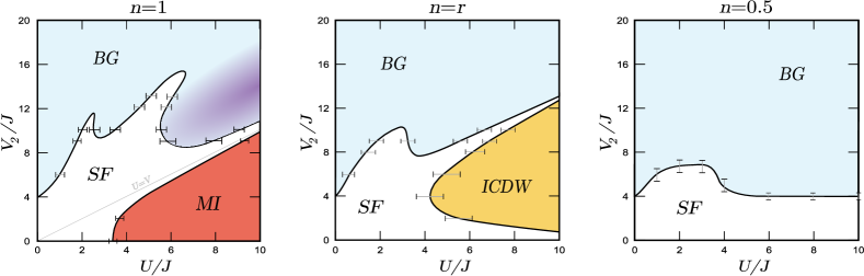
Figure 1: (Color online) Phase diagrams of the bichromatic Bose-Hubbard model for densities $n=1$, $r$ (the ratio of the potential wave lengths) and $n=0.5$. The diagrams are shown as a function of the interaction strength $U$ and the bichromatic potential strength $V_{2}$, both normalized by the hopping $J$ (lines are guides to the eyes). SF stands for the superfluid phase, MI for the Mott-insulating phase, BG for the “Bose-glass” phase (meaning localized but with zero one-particle gap) and ICDW for incommensurate charge-density wave phase. The $U=V_{2}$ line on the phase diagram with $n=1$ indicates the $J=0$ limit for which the gap of the one-particle excitation vanishes. Black error bars are deduced from calculations averaging over the phase-shift $\phi$ (cf. Sec. I.1) and finite-size scaling (see Figs. 12 and 13 for details on the $n=1$ phase diagram). Grey error bars are roughly evaluated from calculations on systems with $L=35$ and fixed $\phi=0$ (see Figs. 11 and 14 for details). In the phase diagram with density $n=1$, the darker (violet) region in the BG phase is localized but could have a small gap which cannot be resolved numerically.

This paper is devoted to the study of the latter situation, the so-called bichromatic set-up, for which experiments have recently been carried out Lye2007 ; Fallani2007 ; Guarrera2007 ; Guarrera2008 . The one-particle Schrödinger equation with an incommensurate lattice has been widely studied Aubry1980 ; Simon1982 ; Thouless1983 ; Kohmoto1983 ; Kohmoto1983a ; Diener2001 and was found to exhibit anomalous diffusion properties Zhong1995 . The main result of these studies, as we will recall later on, is the existence of a critical value of the potential above which localization occurs. For the many-body physics, a weak-coupling treatment of the potential was carried out using bosonization Vidal1999 . Quasi-periodic potentials were found to have an intermediate behavior between commensurate ones, and disordered ones. Exact numerical results on the Bose-Hubbard model with a quasi-periodic potential already exist Roth2003 ; Bar-Gill2006 ; Louis2006 but are limited to small systems and thus could not investigate the nature of the transition nor their precise location. The physics of the Bose-Hubbard model with a periodic superlattice has been investigated Buonsante2004 ; Buonsante2005 ; Rousseau2006 and a “weakly superfluid” phase at large potential depth was found Rousseau2006 . Very recently, Roscilde Roscilde2007 carried out a more detailed study using quantum Monte Carlo calculations and a “random atomic limit” approach. This study gave results on the bulk system for a special choice of parameters, and an accurate description of the physics of the trapped cloud, focusing on static observables. A particularly important point in which we go beyond Ref. Roscilde2007, is the description of the phase diagrams of the bulk system at fixed densities which are essential to understand the interplay between the competing orders at stake.

Our main motivation is to address the shape of these fixed-density phase diagrams for a one-dimensional system using the density-matrix renormalization group (DMRG) algorithm (see section I.3 for details), which results are interpreted within the framework of the Luttinger liquid theory. We focus on the differences and similarities between the deterministic bichromatic lattice potential and a truly random one, usually consisting of a random box distribution (RBD) and for which the phase diagrams without a trap are known Prokofev1998 ; Rapsch1999 . An account of our main results are depicted in Fig. 1, which gathers the phase diagrams for three typical densities as a function of the interaction strength $U$ and the disorder potential strength $V_{2}$ (see Sec. I.1 and Eq. (3) for a precise definition of the hamiltonian). $n$ is the density of bosons and $r$ is the ratio of the employed lattice wave lengths, which characterizes the incommensurability of the potential. A first interesting result is that a finite $V_{2}\geq 4$ is always required to stabilize the BG phase. We must precise that the term BG is used to call a localized phase which is compressible (with a zero one-particle gap), but the detailed features of the BG phase of the bichromatic potential differ from the usual RBD BG phase as will be discussed in what follows. Contrary to the RBD phase diagram, we argue, based on numerical evidence, that there is no intervening BG phase between the SF and the MI phase at density $n=1$. An incommensurate charge-density wave (ICDW) phase – referred to as the incommensurate band insulator (IBI) phase in Ref. Roscilde2007, – emerges at finite $V_{2}$ for a density $n\simeq r$. Lastly, we observe that the larger the density, the larger the extension of the SF phase is.

The paper is organized as follows: in section I, we first give the conditions under which the hamiltonian describing the many-body physics simplifies into a simple lattice hamiltonian used for numerical calculations. We then discuss one of the strongest differences compared to a random box distribution which is the emergence of plateaus in the density-chemical potential curve (section II). We next discuss, in section III, the competition between the disorder potential and the interactions by computing the phase diagrams at integer density one and for a density for which an ICDW plateau occurs. Lastly, section IV is dedicated to the possible relevant experimental probes of localization by focusing on the out-of-equilibrium dynamics of the system.

I The Bose-Hubbard model with an incommensurate superlattice

I.1 Energy scales hierarchy: Validity of the model

This section gives qualitative arguments on the hierarchy of energy scales which leads to a simple lattice hamiltonian that captures the physics of cold bosonic atoms experiencing two optical lattice potentials with wave vectors $k_{1},k_{2}$ and amplitudes $V_{1},V_{2}$. Similar considerations were given recently in Ref. Guarrera2007, . For the sake of clarity, we keep the following discussion on the regime of experimental parameters under which the lattice hamiltonian under study is valid. The potential energy in a one-dimensional setup of two standing-waves is the Harper potential

$$V(x)=V_{1}\cos^{2}(k_{1}x)+V_{2}\cos^{2}(k_{2}x+\phi)\;,$$ (1)

which is sketched in Fig. 2. A constant phase $\phi$ is introduced to shift the second lattice with respect to the other, and the wave vectors $k_{1}$ and $k_{2}$ can take any value. We work in the limit of a large depth $V_{1}\gg E_{r1}$ for which we can restrict ourselves to the lowest Bloch band ($E_{r1}=(\hbar k_{1})^{2}/2M$ is the recoil energy associated with the first lattice and $M$ is the mass of the atoms) and in a situation where one intensity is much larger than the other, $V_{1}\gg V_{2}$. An exact derivation of the lattice parameters of the hamiltonian should resort to numerical calculations as described in Refs. Damski2003, ; Roscilde2007, . Our motivation is to evaluate the physical effect of the perturbing potential to deduce the relative magnitudes of the different terms.

To proceed, we neglect the effect of the trap on the local chemical potential and displacements, meaning that we consider the realistic situation for the bulk physics with $\lambda_{1}\lambda_{2}/|\lambda_{1}-\lambda_{2}|,\lambda_{1},\lambda_{2}\ll\sqrt{\hbar/M\omega}$ with $\omega$ the trap frequency. If $V_{2}=0$, the effective model is the Bose-Hubbard model Bloch2007 with hopping $J_{0}$ and on-site interaction $U_{0}$

$$\mathcal{H}_{0}=-J_{0}\sum_{j}[b^{{\dagger}}_{j+1}b_{j}+b^{{\dagger}}_{j}b_{j+1}]+U_{0}\sum_{j}n_{j}(n_{j}-1)/2\,.$$ (2)

$b^{{\dagger}}_{j}$ is the operator that creates a boson at site $j$ corresponding to the minimum of the lattice potential. The local particle number operator reads $n_{j}=b^{{\dagger}}_{j}b_{j}$. The dependence of the parameters $J_{0}$ and $U_{0}$ upon $V_{1},E_{r1},k_{1}$ and the scattering length $a$ can be evaluated numerically or analytically in this limit Bloch2007 . We now qualitatively discuss the effect of $V_{2}(x)$ to the lowest order in $\varepsilon=V_{2}/V_{1}$.

Perturbation of the chemical potential – First, to zeroth order in $\varepsilon$, the minima of $V(x)$ are located at $k_{1}x_{j}=\pi j+\pi/2$ with $j$ integer and $\pi/2$ can be absorbed in the redefinition of $\phi$. Since $V_{1}(x_{j})=0+O(\varepsilon^{2})$, we have:

$$V(x_{j})=V_{2}\cos^{2}\left(r\pi j+\phi\right)=\varepsilon\frac{V_{1}}{2}[1+\cos\left(2r\pi j+2\phi\right)]$$

The important number which characterizes this bichromatic potential is the ratio of the wave vectors $r=k_{2}/k_{1}$. If $r$ is a rational number $p/q$, the hamiltonian is $q$-periodic. For $r$ irrational, it has no translational invariance and the $V(x_{j})$ can take any value in $[0,V_{2}]$ in a deterministic way: the resulting bounded distribution is sketched in Fig. 2. The chemical potential thus shares features with a one-dimensional quasi-crystal. The order of magnitude of the coefficient of this term is of course $V_{2}=\varepsilon V_{1}$. This term can be larger than $J_{0}$ or $U_{0}$, even though $\varepsilon\ll 1$, because of the factor $V_{1}$. Taking the parameters of Ref. Lye2007, , one finds that $\varepsilon\simeq 0.003$–0.12 while $V_{2}/J_{0}\simeq 2.6$–53.3.

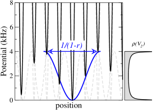
Figure 2: (Color online) The bichromatic potential (full line) with the same parameters as in the experiment of Ref. Lye2007, . Dashed lines show the two beating standing waves from which the bichromatic potential originates. We observe that not only the depths of the potential wells fluctuate but so do their positions and their width. The energetic landscape displays wells of typical width $1/(1-r)$. The plot on the right-hand side shows the bounded distribution which behaves as $1/\sqrt{x(V_{2}-x)}$ and is thus peaked around 0 and $V_{2}$.

Perturbation of the hopping – It is difficult to treat the perturbation of the hopping exactly because one needs to know the non-trivial shape of the perturbed Wannier functions. However, we expect the hopping to be perturbed mainly because of the displacement of the local minima and because tunneling depends exponentially on the distance. We only consider the term associated with the perturbation of the minima $x_{j}$ and $x_{j+1}$ and assume a typical exponential dependence Bloch2007 for the hopping $J_{j,j+1}\sim e^{-h(x_{j+1}-x_{j})}$ with $h=\frac{k_{1}}{2}\sqrt{\frac{V_{1}}{E_{r}}}$, valid for $V_{1}\gg E_{r1}$. The modulation induces a slight fluctuation $\delta x_{j}$ at site $j$ which, to the lowest order in $\varepsilon$, reads:

$$\delta x_{j}=-\frac{1}{2k_{1}}\varepsilon r\sin\left(2r\pi j+2\phi\right)\;,$$

so that the distance between two neighboring sites is altered as:

$$x_{j+1}-x_{j}=\frac{\pi}{k_{1}}-\varepsilon\frac{r}{k_{1}}\sin(\pi r)\cos\left(r\pi(2j+1)+2\phi\right)\;.$$

Hence, to the lowest order in $\varepsilon$, we may write for this term:

$$J_{j,j+1}=J_{0}\left[1+\varepsilon A\cos\left(r\pi(2j+1)+2\phi\right)\right]$$

with, up to approximations, $A=\sqrt{\frac{V_{1}}{E_{r1}}}\frac{r}{2}\sin(\pi r)$. We write $J_{2}=\varepsilon AJ_{0}$. Even though $A$ could be large because of $\sqrt{V_{1}/E_{r1}}$, the factor $\varepsilon$ ensures that $J_{2}$ can be made much smaller than $J_{0}$. More precisely, taking the parameters of Ref. Lye2007, and using the above approximation, one finds $J_{2}/J_{0}\simeq 0.002$–0.1, the latter occurring for very large $V_{2}$, much larger than the ones used in this paper. Numerical calculations of the hamiltonian parameters Damski2003 ; Roscilde2007 confirm that the magnitude of $J_{2}$ is small within our approximations. Hence, we will shorten the notation to $J\equiv J_{0}$ from now on. Another feature which results from this approximation is that the $J_{j,j+1}$ have the same typical fluctuations $\cos(2\pi rj)$ as the $V(x_{j})$ which is observed numerically in Ref. Roscilde2007, , yet for rather large $\varepsilon$.

Perturbation of the local interaction – In the deep well limit, the bare interaction $U_{0}$ is obtained by the relation Bloch2007 :

$$U_{0}=\sqrt{\frac{8}{\pi}}k_{1}aE_{r1}\left(\frac{V_{1}}{E_{r1}}\right)^{3/4}$$

where $a$ is the scattering length. Note that the ratio $U_{0}/J_{0}\sim\exp(2\sqrt{V_{1}/E_{r1}})$ increases exponentially with the lattice depth Bloch2007 . This result can be obtained by approximating the bottom of the cosines with a parabola and using gaussian Wannier functions as the simplest approximation. The fact that $U_{0}$ increases with $V_{1}$ simply corresponds to the squeezing of the parabola. This squeezing may also be changed at first order by $V_{2}$. To give a rough estimate, we can compute the second derivative of Eq. (1) and obtain for the on-site interaction:

$$U_{0}+U_{2}\cos(2r\pi j+2\phi)\text{ with }U_{2}=\frac{3}{4}\varepsilon r^{2}U_{0}\;.$$

Here again, since $\varepsilon$ can be tuned to be very small, one can work within the $U_{2}\ll U_{0}$ regime. The perturbation of the on-site interaction can thus be neglected and we will use the shorter notation $U\equiv U_{0}$ in the following. We also note that the fluctuations of the local interactions have roughly the same cosine dependence as the chemical potential.

To conclude, in the deep well limit $V_{1}\gg E_{r1}$, the following hierarchy of energy scales

$$J_{2},U_{2}\ll U_{0},J_{0},V_{2}\ll V_{1}$$

can be realized experimentally. Thus, we assume the corresponding lattice model for the bichromatic optical lattice:

$$\mathcal{H} = -J\sum_{j}[b^{{\dagger}}_{j+1}b_{j}+\text{h.c.}]+U\sum_{j}n_{j}(n_{j}-1)/2$$ (3)

$$+\frac{V_{2}}{2}\sum_{j}[1+\cos\left(2r\pi j+2\phi\right)]n_{j}$$

$$+\frac{\omega^{2}}{2}\sum_{j}(j-j_{0})^{2}n_{j}$$

with $j_{0}=(L+1)/2$ the center of the trap. In what follows, results for the phase diagrams are computed with $\omega=0$. The trap confinement is added in a few illustrating figures and more importantly, for the preparation of the out-of-equilibrium state in the study of dynamics (Sec. IV).

We can briefly comment on the distribution of the on-site potential energies as it is the first difference with the RBD. We shall use the short-hand notation for the bichromatic potential $V_{2}(x_{j})\equiv V_{j}=V_{2}[1+\cos(2r\pi j+2\phi)]/2$. The distribution of the $V_{j}$ with an irrational $r$ behaves as $1/\sqrt{x(V_{2}-x)}$ which diverges close to 0 and $V_{2}$ and is symmetrical with respect to $V_{2}/2$ (see Fig. 2) but is relatively flat at the center. Thus, this distribution qualitatively lies in between a RBD and a binary one. Its auto-correlation function reads:

$$\overline{V_{j}V_{j+d}}-\overline{V_{j}}^{2}=(V_{2})^{2}\cos(2\pi rd+2\phi)/8$$

where the over-bar means averaging over all sites $j$. The potential is thus deterministic and correlated. Though trivial, this remark stresses the fact that the very features of the localization mechanism under study originates from the quasi-periodicity rather than the distribution itself. For instance, an uncorrelated disordered potential with the same distribution would induce localization as soon $V_{2}$ is finite, which is not true for the bichromatic one. As sketched in Fig. 2 by black and dashed grey lines, wells develop over a characteristic length scale $1/(1-r)\simeq 4.4$ sites which comes from the beating of the two periods 1 and $r$ of the two lasers.

Working with finite systems raises the question of taking the thermodynamical limit. The system length $L$ is given in units of the first lattice spacing $\lambda_{1}/2$. First, to what extent can an irrational number $r$ be approximated by a rational number? This can be answered by looking at its continuous fraction decomposition wikicontinuedfraction which gives the successive best rational approximations. From Ref. Lye2007, , $r=830.7/1076.8=0.77145245\ldots$ is a realistic “irrational” parameter as 8307 and 10768 are coprimes. The successive best rational approximations are $3/4,7/9,10/13,17/22,27/35,908/1177,\ldots$ which gives the lengths $L=13,22,35,1177$, best “fitting” the potential for non-trapped systems. As $27/35$ is already a fairly good approximation of the “irrational” $r$ of the experiments, multiples of 35 such as 70, 105, can be used as well. We will also use other lengths $L$ and we have checked that the physics does not change qualitatively if the system size does not perfectly fit the potential. The fact that 35 is a rather large period ensures that $r$ is not too close to a simple fraction which would induce strong commensurability effects on finite systems. In what follows, we choose to work with the experimental parameter $r=0.77145245$ as Roscilde did Roscilde2007 to be as close as possible to the experiments but we expect the general picture to remain true for any irrational number. Furthermore a phase shift $\phi$ enters in the hamiltonian and, though we expect the potential to be self-averaging for fixed $\phi$, averaging over $\phi$ can help recover the thermodynamical limit. This averaging will be denoted by $\langle{}\rangle_{\phi}$ in the following. As experimental set-ups generally consist in an assembly of one-dimensional cigar-shaped clouds with different lengths (see Fig. 3 of Ref. Fallani2007, for instance), clouds with different lengths would effectively experience a different phase shift $\phi$. Furthermore, from one shot to another, the tubes experience slightly different potentials. This is due to the difficulty to lock the position of the cloud in the trapping and optical lattice potentials over several shots. Consequently, $\phi$ may fluctuate from one preparation to another.

The last crucial parameter in the physics of the system is the density which plays an important role as we will see. For a non-trapped system, we use the notation $n=N/L$ with $N$ the total number of bosons which is kept fixed as we work in the canonical ensemble. For a trapped system, the local density varies as one moves away from the middle of the trap and the thermodynamical limit is recovered for $\omega\rightarrow 0$ keeping $N\sqrt{\omega}$ constant. Roscilde Roscilde2007 gave a detailed analysis of the static properties in the presence of a trap. Our focus is more on the phase diagram of the model which is always understood to be in the thermodynamical limit. More details with respect to experimental probing will be given in section IV. All results of the paper are for zero temperature.

I.2 Low-energy approach: bosonization

We briefly review known results from the low-energy approach (close to a hydrodynamic description) which will be useful for the interpretation of the numerics and offer a complementary point of view on the physics. The low-energy physics of interacting bosons in 1D are described using Haldane’s harmonic fluid approach Haldane1981 ; Cazalilla2004 ; Giamarchi2004 in which the density operator is expanded as:

$$\rho(x)=\left[n-\frac{1}{\pi}\nabla\phi(x)\right]\sum_{p=0,\pm 1,\pm 2,\ldots}e^{ip(2\pi nx-2\phi(x))}$$ (4)

where $n$ is the boson density which encompasses the lattice spacing $d$. The effective hamiltonian of the system has generically a quadratic part which includes a kinetic energy term $\sim\Pi^{2}$, with $\Pi=\frac{1}{\pi}\nabla\theta$ the conjugate field of $\phi$ (the commutation relations $[\phi(x),\Pi(x^{\prime})]=i\delta(x-x^{\prime})$ and $[\theta(x),\frac{1}{\pi}\nabla\phi(x^{\prime})]=i\delta(x-x^{\prime})$ hold), and a density-density like interaction term $\sim(\nabla\phi)^{2}$. Two Luttinger parameters $u$ and $K$ give a simple parameterization of the quadratic part of the hamiltonian:

$$\mathcal{H}=\int\frac{dx}{2\pi}\left\{uK(\pi\Pi)^{2}+\frac{u}{K}(\nabla\phi)^{2}\right\}$$ (5)

where $u$ has the dimension of a velocity and $K$ is dimensionless. For free bosons, only the first term remains which would formally correspond to the $K\rightarrow\infty$ limit and $u=\sqrt{n\pi/M}$ is the sound velocity. Taking into account a local interaction $\frac{U}{2}\rho(x)^{2}$ like in the Bose-Hubbard model, the Luttinger parameters read $u=\sqrt{nU/M}$ and $K=\pi\sqrt{n/MU}$ in the limit $U\ll J$. When interactions are large, higher harmonics in the density operator have to be taken into account to describe correctly the local fluctuations and not only the long-distance ones. In the $U=\infty$ limit, i.e. for hard-core bosons (HCB), one obtains $K=1$ as one would find for free fermions. The strong interaction, i.e. the second term in Eq. (5), acts as a Pauli exclusion term. We thus generically have $1\leq K<\infty$ for on-site repulsive interactions. The effective hamiltonian (5) provides the general low-energy description of the SF phase which can undergo various instabilities.

By bosonizing the standard Bose-Hubbard model (2), commensurability effects can arise from the higher harmonics Giamarchi2004 :

$$\rho(x)^{2}=n^{2}+\frac{1}{\pi^{2}}(\nabla\phi)^{2}+n^{2}\sum_{p>1}\cos[2\pi pnx-2p\phi(x)]+\ldots$$

¿From studying the renormalization group (RG) flow equations, it is known that cosine terms such as

$$U\int dx\cos[2\pi pnx-2p\phi(x)]$$ (6)

can lock the density field $\phi$ and induce a commensurate-incommensurate transition Dzhaparidze1978 (C-IC) depending on the density and of $K$. Working at fixed density and varying interactions, such a term is relevant only if the density satisfies the commensurability condition $pn=1,2,\ldots$ and if $K<K_{c}$ with $K_{c}=2/p^{2}$. The opening of the gap follows a Kosterlitz-Thouless Kosterlitz1973 (KT) law $\Delta_{c}\sim\exp(-A/\sqrt{U-U_{c}})$ with $A$ a constant and $U_{c}$ the critical value. Working at fixed interaction and varying the density, the commensurate phase is obtained for $K_{c}=1/p^{2}$. For instance, for $p=1$, integer densities $n=1,2,3,\ldots$ allow for a Mott phase for $K$ below $K_{c}=2$. For $p=2$, charge-density wave phases can appear for half-integer densities but nearest-neighbor repulsion are required Giamarchi2004 ; Giamarchi1997 ; Kuhner2000 to get $K<1$. It is important to note that such cosine effective potential terms effectively arise from the interactions. The transition towards the charge density-wave (CDW) state with one atom every two sites Kuhner2000 is associated with a spontaneous breaking of the translational symmetry. The other possibility to generate Mott phases is to artificially introduce a cosine chemical potential which directly couples to the density. Similarly, a CDW phase induced by an external potential is associated with an explicit breaking of the translational symmetry. This latter solution is possible in cold atoms by adding a superlattice.

Effect of a superlattice potential – We first consider a cosine potential $V_{2}(x)=V_{2}\cos(Qx)$ which has only one Fourier component at wave vector $Q=2\pi r$ with $r$ rational. The additional term reads

$$\int dxV_{2}(x)\rho(x)=\frac{V_{2}}{2}\int dx\cos[(2\pi n\pm Q)x-2\phi(x)]+\ldots$$ (7)

As seen previously, such terms may induce a C-IC transition when increasing $V_{2}$ if the condition $n\pm r\in\mathbb{Z}$ is satisfied. In particular, the superlattice potential can become relevant for the densities $n=r,1-r,1+r,2-r,\ldots$. Higher harmonics can be generated, as discussed in Sec. II.1. If the potential term is not relevant, the Luttinger parameter $K$ is, however, renormalized to a lower value by the potential as it happens with interactions. Such commensurate potentials have for instance been studied in the context of Mott transitions Giamarchi1997 and of magnetization plateaus Arlego2001 . The physics of cold atoms with induced commensurate CDW phases was studied in detail in Ref. Rousseau2006, . Vidal et al. Vidal1999 generalized this result to irrational $r$. For the case of a quasi-periodic potential, the critical value $K_{c}$ remains equal to 2 if the density approximately satisfies the relation $n\pm r\in\mathbb{Z}$. If the density does not fulfil this condition but remains close enough, an insulating phase can be reached but for smaller critical value (for a spin-less fermion model, $K_{c}\simeq 1$ was found from RG).

Disorder with a random box distribution – From Refs. Giamarchi1987 ; Giamarchi1988 ; Fisher1989 , the main result is that the potential is relevant below the critical value $K_{c}=3/2$, whatever the density. The resulting Bose-glass phase has no one-particle gap but an exponentially decaying one-particle Green’s function due to localization. The correlation length scales according to $\xi\sim\exp(-A/(V_{2}-V_{2}^{c}))$ where $V_{2}^{c}$ is the critical value for the transition.

I.3 Numerical methods

The hard-core bosons physics can be solved exactly using a Jordan-Wigner transformation which maps the model onto free fermions with boundary conditions that depend on the number of bosons. As the method has been widely described in the literature, we refer the reader to Refs. Rigol2005 ; Roscilde2007 . This method is also used to investigate the out-of-equilibrium properties Rigol2005 of the cloud in section IV.

We use the DMRG algorithm White1992 ; White1993 ; Schollwoeck2005 to treat the soft-core Bose-Hubbard model (3). For disordered systems, sweeping has proven to be particularly important to get reliable results Schmitteckert1998 ; Rapsch1999 . DMRG has also been used to investigate the physics of quasi-periodic electronic systems Hida2001 ; Schuster2002 . Our implementation is based on a matrix-product state variational formulation McCulloch2007 which enables us to start sweeping from any state. In practice, we have started from either a random or a classical state (where the particles are located according to the $J=0$ limit of the hamiltonian) contrary to the usual warm-up method. The algorithm works in the canonical ensemble (fixed number of particles $N$) and at zero temperature. We typically use from 200 to 400 kept states. The number of bosons allowed on-site is usually fixed to $N^{\text{bos}}=4$ but results for densities larger than one have also been checked with up to $N^{\text{bos}}=6$. For $U\geq 1$ and $V_{2}\leq 20$, the classical distribution of particles does not have more than 4 bosons per sites.

A drawback of this variational method is the occasional tendency to get trapped in an excited (metastable) state with a slightly higher energy that is difficult to distinguish numerically from the ground-state. Indeed, the usual measures of the convergence of DMRG, the discarded weight and the variance $\langle{(\mathcal{H}-E)^{2}}\rangle$ are very small for these states. Systematic tests have been carried out in the $U\rightarrow\infty$ limit. Starting from the classical state improves convergence for small densities or close to one at large $V_{2}$ as one would expect intuitively. Below $V_{2}\simeq 4$, convergence is always good which can be related to the physics of the systems as the potential does not induce localization in this regime. In the case of soft-core bosons, we expect an enhancement of quantum fluctuations at finite $U$ to help the particles redistribute more easily. Such equilibration is rendered very difficult for HCB as for strong $V_{2}$, local densities can be very close to one. Most of the data have been obtained for $U\lesssim V_{2}$. Furthermore, relying on the variational principle, we can use the smallest of the two energies obtained from starting either from the classical or a random state. Lastly, the coherence of the results obtained from observables computed independently, such as the correlation length and the one-particle gap (see section III), supports the good convergence of the algorithm.

II Density plateaus: Mott and incommensurate charge density wave phases

This section describes the relation between the density $n$ and the chemical potential $\mu$ for a non-trapped cloud. The motivation is to find first the location of the compressible and incompressible phases. The chemical potential is computed via

$$\mu(N)=E_{0}(N)-E_{0}(N-1)$$

where $E_{0}(N)$ is the ground-state energy with $N$ bosons. If a plateau emerges in the $n(\mu)$ curve, its width is directly related to the one-particle gap defined by

$$\begin{split}\Delta_{c}&=E_{0}(N+1)+E_{0}(N-1)-2E_{0}(N)\\ &=\mu(N+1)-\mu(N)\end{split}$$

Lastly, the compressibility of the system $\kappa=\partial n/\partial\mu$ is evaluated through its discretized expression as

$$\kappa^{-1}=L[E_{0}(N+1)+E_{0}(N-1)-2E_{0}(N)]\;.$$ (8)

For a Luttinger liquid, the compressibility is simply related to the Luttinger parameter and the sound velocity:

$$\kappa=\frac{K}{\pi u}\;.$$ (9)

The compressibility naturally vanishes in a plateau phase.

II.1 Plateaus in the hard-core boson limit

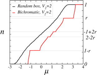
Figure 3: (Color online) Comparison of $n(\mu)$ for a random and a bichromatic potential (irrational $r$) for hard-core bosons. Plateaus open for the bichromatic potential, the main ones being at $n=r$ and $1-r$.

Following Ref. Fisher1989, , setting $J=0$ gives insight into the $J\ll U$ physics. This gives the width $U-\max(V_{j})+\min(V_{j})$ of the various Mott plateaus centered at $\mu/U=0.5,1.5,2.5,\ldots$. This is due to the fact that in the limit $J=0$ one can reorder the energies by increasing values and therefore the $n(\mu)$ curve which is the integrated density of states is simply linear between Mott plateaus for the random box distribution and $U>\max(V_{j})-\min(V_{j})$. For a bichromatic lattice, we have $\mu=V_{2}\sin(\pi n/2)$. What happens when $J$ is small but finite? The density of states evolves smoothly with $J$ for the random box distribution (see Fig. 3). For $V_{2}=0$, the bandwidth which develops between the Mott plateaus has a width $4J$ and a cosine relation can be observed Batrouni1990 because Mott sub-bands with cosine dispersion are well separated. On the contrary, for the bichromatic lattice intermediate plateaus appear as soon as $J$ is non-zero. This behavior is reminiscent of the situation for rational $r$ and was discussed extensively for free fermions, which in our case would be equivalent to the HCB limit.

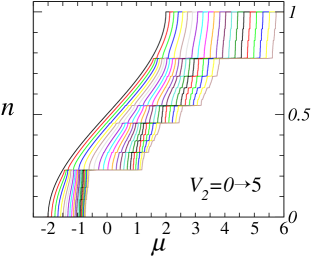
Figure 4: (Color online) Opening of plateaus in the $n(\mu)$ curves with $V_{2}$ for hard-core bosons ($V_{2}$ is increased by steps of $J/4$ and is in units of $J$, as $\mu$). Above the critical value $V_{2}^{c}=4$, the curves acquire a devil’s staircase-like behavior: plateaus become dense.

The energy spectrum and the wave function properties have been widely studied in the literature Aubry1980 ; Simon1982 ; Kohmoto1983 ; Kohmoto1983a ; Thouless1983 ; Barache1994 . It was shown that gaps open in the energy spectrum. If $r$ is rational, there is a finite number of gaps. If $r$ is irrational, there is an infinite number of gaps at large $V_{2}$, the width of which strongly depends on $p$ and $q$ if one writes $n=p/q$ and gets larger as $V_{2}$ increases. We here recall the method usually followed: these gaps are studied by $m$ successive approximations $r_{m}=p_{m}/q_{m}$ of the irrational number $r$. For a given $m$, the potential is $q_{m}$ periodic and we can use Bloch’s theorem on super-cells of length $q_{m}$. The one-particle Schrödinger equation of the hamiltonian (3) reads:

$$-J(\psi_{j+1}+\psi_{j-1})+[V_{j}-E]\psi_{j}=0\,.$$ (10)

Using $V_{j+q_{m}}=V_{j}$ and Bloch’s theorem $\psi_{j+q_{m}}=e^{ikq_{m}}\psi_{j}$, the spectrum is obtained by solving the determinant of size $q_{m}$:

$$\begin{vmatrix}V_{1}-E&-J&&-Je^{-ikq_{m}}\\ -J&V_{2}-E&-J&\\ &-J&\ddots&-J\\ -Je^{ikq_{m}}&&-J&V_{q_{m}}-E\\ \end{vmatrix}=0$$

For $q_{m}=2$, this is the simple band folding mechanism which opens a gap at $n=1/2$, with a doubling of the unit cell. More generally, at most $q_{m}-1$ gaps appear in the spectrum made of $q_{m}$ bands $\mathcal{E}_{1,\ldots,q_{m}}(k)$ with $k\in[-\pi/q_{m},\pi/q_{m}]$. Examples of effective dispersion relations for the bichromatic potential can be found in Sec. IV. Fig. 4 displays the opening of the plateaus for HCB with $V_{2}$. A simple real-space interpretation can be given for the main plateau at $n=1-r$: it amounts to fill each well of size $1/(1-r)$ with one particle (see Fig. 2). The plateau at $n=r$ is simply obtained with the same argument with holes instead of particles. Putting two particles (holes) in each well can lead to plateau at densities $2(1-r)$ and $1-2(1-r)=-1+2r$. The fact that the main plateaus at $n=r,1-r$ develop as soon as $V_{2}$ is turned on is expected from the bosonization arguments of Sec. I.2, since $K(V_{2}=0)=1<K_{c}=2$ for HCB. From a momentum space point of view, these opening are associated with umklapp processes with a momentum transfer $Q$ which, modulo $2\pi$, gives back the conditions $n=r,1-r$. In perturbation theory, processes with larger momentum transfers can be obtained from Eq. (7) with higher order terms in $V_{2}$. For instance, to second order, terms with transfers $2Q$ (corresponding to $n=2-2r$ and $-1+2r$) will appear if $K<1/2$. Consequently, a finite $V_{2}$ is required to stabilize these plateaus (see also Fig. 9). As $V_{2}$ is increased, such processes break the spectrum up and make it point-like for the critical value $V_{2}=4$ which is beyond this weak-coupling bosonization interpretation. Lastly, we note that this is particular to the Harper model. For the Fibonacci chain Vidal1999 , the Fourier transform of the potential is already dense at small $V_{2}$. In our situation, the Fourier spectrum gets denser as $V_{2}$ is increased.

II.2 Plateaus for soft-core bosons

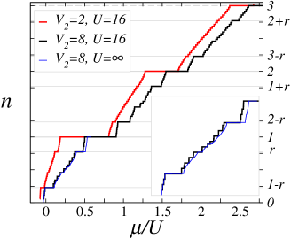
Figure 5: (Color online) $n(\mu)$ for soft-core bosons with a large interaction parameter $U=16$ at small and large $V_{2}$ computed on a system with $L=35$ and a fixed phase-shift $\phi=0$. Inset: curves at low density show the comparison between hard-core bosons ($U=\infty$) and soft-core ones, which is good up to finite size effects.

We now consider the case of a finite interaction $U$. First of all, the hard-core boson limit is likely to give the correct qualitative behavior for large $U$. Indeed, at low densities, an interaction $U$ slightly larger than $V_{2}$ might be sufficient to recover the HCB physics as multiple occupancies are already strongly suppressed. Densities larger than one are allowed for soft-core bosons. For large $U$, we expect to find plateaus in between each Mott plateaus. One may recover the hard-core bosons band folding mechanism inside each Mott sub-bands (or at least for the lowest ones). These simple observations are coherent with the large $U$ numerical data displayed in Fig. 5. A comparison with HCB results is provided in the inset of Fig. 5 which proves that $U=16$ is sufficiently large to reproduce the HCB physics within the first three Mott sub-bands.

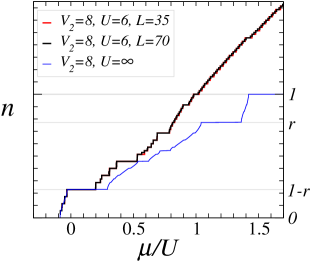
Figure 6: (Color online) Plateaus with a large $V_{2}\sim U$. Some of the largest plateaus found do not correspond to the hard-core boson limit. The two sizes $L=35$ and 70 give an idea of the (weak) finite size effects.

Fig. 6 gathers the results when $U\leq V_{2}$, unveiling a more surprising behavior. As discussed previously, we expect the HCB behavior to account for the low-density part of the curve, which is actually observed through the rather large width of the $n=1-r$ plateau. Indeed, because this plateau corresponds to one particle in each well, the effect of interactions is restricted to virtual processes. For higher densities, a large compressible phase is obtained, manifested by the smooth increase of the density. From a phenomenological point of view, adding atoms fills the well minima. Since $U$ is not too large, the effective potential coming from the combination of the interaction and the superlattice potential gets smoother and smoother. Consequently, the associated gain in kinetic energy favors a compressible and actually a superfluid state as we will see in Sec. III.8 where delocalization by increasing the density is discussed. In between those two regimes, the behavior is non-trivial. Strikingly, some plateaus existing in the HCB limit totally disappear, such as the $n=r$ plateau, while others acquire a larger width. Having gaps whose size increases when interactions are reduced is something rather counter-intuitive. These plateaus result from the interplay of the potential and the interactions. A real-space picture was given by Roscilde Roscilde2007 following a random atomic limit: considering wells of typical size $1/(1-r)$ separately, the fine structure of the energy levels for each number of atoms inside the wells depends strongly on $U,V_{2}$ and also on $J$. Connecting wells with $J$ allows for the computation of the integrated density of states which is $n(\mu)$. Though physically enlightening, this approach is quantitatively correct for rather small densities. Since the observed plateaus stem from the interplay of the interactions and the potential, we call the corresponding plateau phase an incommensurate charge density-wave phase. They appear to be the extension of both the Mott and the incommensurate HCB phases at smaller $U$. Bosonization explains, at least qualitatively, the mechanism of plateaus opening in the HCB limit by considering high order perturbative terms coming from Eq. (7), which gives for instance the first two densities $r,1-r$ and $2(1-r),-1+2r$. At finite $U$ and when $U\sim V_{2}$, the situation is more involved as both terms should be treated non-perturbatively and on an equal footing. Predicting the observed densities at which these ICDW phases occur is thus beyond the perturbative approach.

III Localization induced by interactions or disorder: Phase diagrams

We have seen that contrary to the standard random box situation, there is not only one phase (either the BG or the SF) between the MI phases but a succession of phase transitions as the chemical potential is increased. This renders the usual Fisher1989 interpretation of the phase diagram in the $(\mu,J/U)$ plane for a fixed ratio $V_{2}/U$ rather strenuous Roscilde2007 as the succession of phase transitions breaks it up into many compressible and incompressible pieces. Thus, we prefer to work at fixed density and varying the two competing parameters $V_{2}/J$ and $U/J$. These phase diagrams were first sketched numerically in Refs. Roth2003 ; Louis2006 ; Bar-Gill2006 but on very small systems and without a discussion of the boundaries and the nature of the transitions. We here provide a more precise determination, in particular, by using scaling over different sizes and averaging over $\phi$ when necessary. We now describe more precisely the various observables used to sort out the phases.

III.1 Observables

In addition to the compressibility, we need further observables to sort out the different phases realized in the bichromatic set-up. The first natural one is the superfluid density $\rho_{s}$. It can be computed using twisted boundary conditions:

$$\rho_{s}=2\pi L\frac{E_{0}^{\text{apbc}}-E_{0}^{\text{pbc}}}{\pi^{2}}$$ (11)

where the ground-state energies are computed for periodic (pbc) and anti-periodic (apbc) boundary conditions. With this definition, $\rho_{s}$ actually matches the superfluid stiffness. Other definitions Rapsch1999 contain the density of particles $n$ as a prefactor. The superfluid density is zero in the BG, ICDW and MI phases and finite only for the SF phases. In a Luttinger liquid, the superfluid density is directly related to the Luttinger parameters through

$$\rho_{s}=uK\;.$$ (12)

Combined with Eq. (9), $K$ can then be computed using $K=\sqrt{\pi\rho_{s}\kappa}$. This numerical evaluation only requires the calculation of energies. $K$ can be independently extracted from correlation functions. For instance, the one-particle density-matrix or bosonic Green’s function reads $\langle{b^{{\dagger}}_{i}b_{j}}\rangle$ where $\langle{}\rangle$ indicates the expectation value in the ground-state. Following Ref. Kollath2004, , we extract the contribution of the phase $\theta(x)$ fluctuations by dividing it by the local inhomogeneous densities $n_{i}$:

$$G(|{i-j}|)=\frac{\langle{b^{{\dagger}}_{i}b_{j}}\rangle}{\sqrt{n_{i}n_{j}}}\;.$$ (13)

The motivation for this renormalization stems from the observation that the density-phase expression of the boson creation operator is $b_{i}=\sqrt{\rho(x_{i})}e^{-i\theta(x_{i})}$, and the fact that the correlator which features superfluid properties in bosonization is $\langle{e^{i\theta(x_{i})}e^{-i\theta(x_{j})}}\rangle$. For a translationally invariant model, both definitions only differ by a constant factor. Since there is no translational invariance, one must likewise average correlations over all couples of points with the same distance $x=|{i-j}|$ to obtain a smooth behavior for this correlation. A typical plot is given in Fig. 20. In the case of the BG, ICDW or MI phases, the Green’s function decays exponentially $G(x)\propto e^{-x/\xi}$. In the Mott phase, the correlation length $\xi$ goes as the inverse one-particle gap $\xi\sim 1/\Delta_{c}$. An effective correlation length can also be computed on a finite system using Kuhner2000 :

$$\xi^{2}(L)=\frac{\sum_{x}x^{2}G(x)}{\sum_{x}G(x)}\;.$$ (14)

This gives a correct estimate of the correlation length for the localized phases in the thermodynamical limit up to a factor $\sqrt{2}$. A divergence of $\xi$ with $L$ signals a superfluid state in which the asymptotic behavior of the Green’s function is algebraic with an exponent controlled only by the parameter $K$

$$G(x)\propto\frac{1}{\displaystyle x^{1/2K}}\;.$$ (15)

This allows for the evaluation of $K$ by using an accurate fitting procedure on a finite system with open boundary conditions. This is briefly described in Appendix A.

Characterizing the Bose condensation of the cloud is often done by looking at the condensate fraction $f_{c}$. It is usually computed on finite clusters as the largest eigenvalue of the matrix $\rho_{ij}=\langle{b^{{\dagger}}_{j}b_{i}}\rangle$. No average over sites nor normalization by the local density is performed here. The largest possible value $f_{c}$ can reach is the number of bosons $N$. In the limit of HCB, quasi-condensation results in the scaling $f_{c}(N)\propto\sqrt{N}$. A finite $f_{c}$ is a feature of either the BG, the ICDW or the MI phase. Experimentally, time-of-flight measurements are related to the Fourier transform of $\rho_{ij}$, namely

$$n(k)=\frac{1}{L}\sum_{lm}e^{ik(l-m)}\rho_{lm}\;.$$ (16)

Coherence of the quantum gas is deduced from the appearance of a narrow central peak $n(k=0)$.

III.2 Localization of free bosons

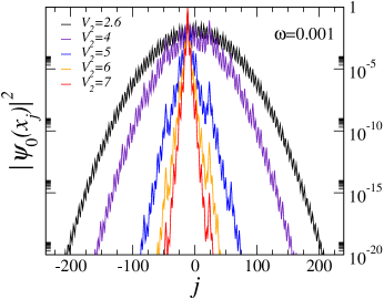
Figure 7: (Color online) Ground-state wave function of the lattice model (3) with a smooth trap but no interaction for increasing perturbing potential $V_{2}$. There is a crossover from a gaussian wave function (log scale) to an exponential one. Note that the maximum of the wave function in the presence of strong $V_{2}$ is not centered at the middle of the trap.

We start with the simplest situation of free bosons, the $U=0$ limit, in which all bosons lie in the ground-state single particle wave function $\left|{\psi_{0}}\right\rangle$. In Fig. 1 of Ref. Lye2007, , the structure of the trapped wave function is obtained from the Gross-Pitaevskii equation. Similar results are found here for the lattice model (3) as shown in Fig. 7 which displays the qualitative change of shape from a gaussian to an exponential structure. In order to quantify the localization transition of a single-particle wave function $\left|{\psi}\right\rangle$, one can use the inverse participation ratio which is usually defined as

$$I(\psi)=\sum_{j}|{\left\langle{\psi}|{j}\right\rangle}|^{4}\;.$$ (17)

$\left|{j}\right\rangle$ is the state at site $j$ in the real space basis. In the thermodynamical limit, $I(\psi)$ goes to zero for a delocalized state with a typical scaling $1/L$ or $\sqrt{\omega}$ for respectively a non-trapped and a trapped system, while it remains constant for a localized wave function. Based on an exact duality transformation of the one-particle Schrödinger equation (10), the localization of the wave function has been conjectured by Aubry and André Aubry1980 to happen at the critical value $V_{2}^{c}=4$. This conjecture is illustrated in Fig. 8 which displays $\langle{I(\psi_{0})}\rangle_{\phi}$ as a function of $V_{2}$. In comparison with the RBD evolution, the bichromatic set-up displays a sharp transition even for a finite trap frequency provided it is small enough. For the RBD, localization occurs as soon as $V_{2}\neq 0$ Abrahams1979 with a typical scaling $I(\psi_{0})\sim\sqrt{V_{2}}$.

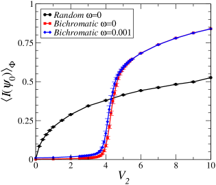
Figure 8: (Color online) The averaged inverse participation ratio $\langle{I(\psi_{0})}\rangle_{\phi}$ as a function of $V_{2}$ for a bichromatic lattice and a random box distribution. There is a sharp transition at $V_{2}^{c}=4$ in the thermodynamical limit ($L=420$ for $\omega=0$). A similar sharp transition is also found for the system with a smooth trap.

III.3 Localization of hard-core bosons

We have seen that plateaus emerge in the $n(\mu)$ curve as soon as $V_{2}$ is turned on and that the spectrum is point-like above $V_{2}^{c}=4$. The extension of the wave functions is related to the nature of the energy spectrum and it was shown Aubry1980 ; Simon1982 that all wave-functions are extended below $V_{2}^{c}$ while they are all localized above. Consequently, we expect the HCB to localize above $V_{2}^{c}$, whatever the density. Below $V_{2}^{c}$, HCB can be either in a SF or in an ICDW state. To illustrate this situation, we plot in Fig. 9 the behavior of the Luttinger exponent $K$ as a function of $V_{2}$ and the density $n$. It nicely shows that $K=1$ in superfluid phases as expected for HCB but vanishes (up to finite size effects) for the densities corresponding to the ICDW phases, the main ones being located at $n=r$ and $1-r$. Many gaps develop as the critical point is approached and the shrinking of the bands renders the low-energy approximation and calculation of $K$ difficult close to this point.

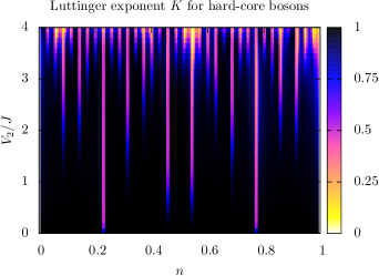
Figure 9: (Color online) The Luttinger parameter $K$ for hard-core bosons as a function of $V_{2}$ and the density $n$ on a finite system with $L=175$ for an irrational $r=0.7714\ldots$. Strictly speaking, $K$ should be equal to 1 in all superfluid phases and 0 in the gapped phases. Up to finite size effects, vertical bands reveal the successive openings of gaps as $V_{2}$ is increased.

As a partial conclusion, the two limiting cases $U=0$ and $U=\infty$ of the $(U,V_{2})$ phase diagrams of Fig. 1 can be summed up as follow: (i) for a generic density $n$ (meaning that it does not correspond to an ICDW plateau) and also for the $U=0$ limit whatever the density, the system remains superfluid for $V_{2}<4$ and localizes in a BG phase for $V_{2}>4$ with a correlation length which behaves according to $\xi^{-1}\sim\ln(V_{2}/4)$ Aubry1980 ; Simon1982 ; Thouless1983 , (ii) for a density close to a plateau phase (for instance $n=r$ or $1-r$) and $U=\infty$, there is a transition towards an ICDW phase for a critical value of $V_{2}$ which is smaller than 4 (and precisely equal to 0 for $n=r$ or $1-r$), (iii) for the commensurate integer density $n=1$ and $U=\infty$, the system remains in the MI phase ground-state for any $V_{2}$.

III.4 The superfluid – Bose glass transition for soft-core bosons

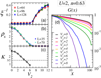
Figure 10: (Color online) Superfluid-Bose glass localization transition. The parameters $U=2$ and $n=0.63$ are chosen such that the system is in the superfluid phase at $V_{2}=0$. (a) The inverse correlation length scales roughly as $\sqrt{V_{2}-V_{2}^{c}}$ where $V_{2}^{c}=6.9$ is much larger than the non-interacting critical value $V_{2}^{c}=4$. Below $V_{2}^{c}$, we have the scaling $\xi\sim L$ typical of a superfluid state. (b) $\rho_{s}$ provides an independent determination of the transition. (c) Evolution of the Luttinger exponent $K$ as a function of $V_{2}$. The dashed line displays the RBD result $K_{c}=3/2$. (d) Averaged one-particle density-matrix $G(x)$ for increasing $V_{2}$ showing the transition from an algebraic to an exponential decay.

We address here the direct transition from the SF to the BG phase which occurs for a generic density by increasing the strength of the potential $V_{2}$. Fig. 10 provides the evolution of the Green’s function $G(x)$ showing the localization transition. First, a finite “disorder” strength with a critical value $V_{2}^{c}\simeq 6.9$ is necessary to obtain exponentially decaying correlations. This value is larger than the $U=0$ and $U=\infty$ limits; interactions have a delocalization effect on the BG phase similarly to the RBD box results. Qualitatively, this can be understood by starting from the localized state. There, the condensate is fragmented into pieces. Repulsive interactions will make the condensate fragments inflate and, by doing so, will help make them overlap and build coherence. For bosons, interactions thus helps delocalization. Interestingly, computing the Luttinger exponent from the correlations shows that the critical value $K_{c}$ at the transition is smaller than the RBD result $3/2$. The scaling properties of the transition thus differ from the standard SF-BG transition. Finding a $K_{c}$ smaller than the RBD result for the Harper potential is well compatible with the analytical finding for $K$ found for the Fibonacci potential in Refs. Vidal1999, .

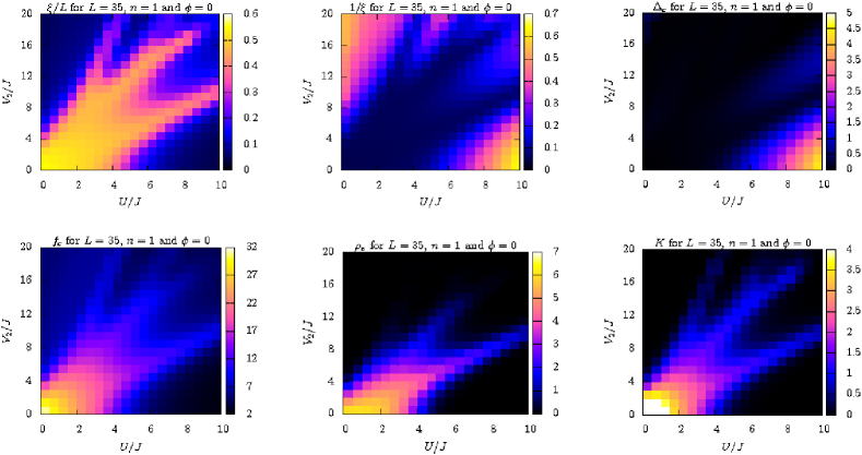
Figure 11: (Color online) Phase diagram for $n=1$. Observables are computed with DMRG for a system with $L=35$ and fixed phase-shift $\phi=0$ as a function of $U$ and $V_{2}$. The $V_{2}=0$ line shows the Mott transition at $U_{c}=3.3$ while the $U=0$ line shows the free boson localization transition around $V_{2}^{c}=4$. The Mott insulating phase gets qualitatively delocalized as $V_{2}$ increases for $U$ not too large. Increasing $U$ delocalizes the BG phase if $V_{2}$ is not too large.

To proceed with the discussion of the competition between interactions and the disordered potential, we compute with DMRG the phase diagrams of the system in the three generic cases $n=1$ (competition between the SF, Mott and BG phases), $n\simeq r$ (competition between the SF, ICDW and BG phases), and lastly $n=0.5$ (competition between the SF and BG phases only). The summary of the phase diagrams is given in Fig. 1.

III.5 Phase diagram at $n=1$

All observables relevant for the construction of the phase diagram as a function of the interaction $U$ and the potential depth $V_{2}$ are reported in Fig. 11 for the integer density $n=1$. The Mott phase is characterized by a finite gap $\Delta_{c}\sim 1/\xi$, a zero SF density and a finite and small (of order unity) condensate fraction. It emerges at the bottom right corner above the critical value Kuhner2000 $U_{c}\simeq 3.3$ for $V_{2}=0$. We observe that $U_{c}$ increases with $V_{2}$ as for the RBD, meaning that $V_{2}$ destabilizes the Mott phase. One can understand from a simple local on-site energies argument: the disorder reduces the minimum one-particle energy gap in the atomic limit. The BG phase exhibits exponentially decaying correlations, a zero SF density and a non-diverging condensate fraction but no gap. It emerges for large $V_{2}$ region of the $V_{2}>U$ half-part of the phase diagram. Note that the BG has a condensate fraction $f_{c}$ that is slightly larger than for the MI phase, qualitatively due to the fact that coherence should remain significant over the typical length scale of the wells, namely $1/(1-r)$. The SF phase has a finite SF density but no gap and algebraic correlations. It generically emerges at low $U$ and low $V_{2}$ and surprisingly extends into a hand print like pattern. A very small (compared to $U$ and $V_{2}$) one-particle gap is observed for large $U$ and large $V_{2}$ but we cannot conclude whether it is a finite size effect or not (see Fig. 13).

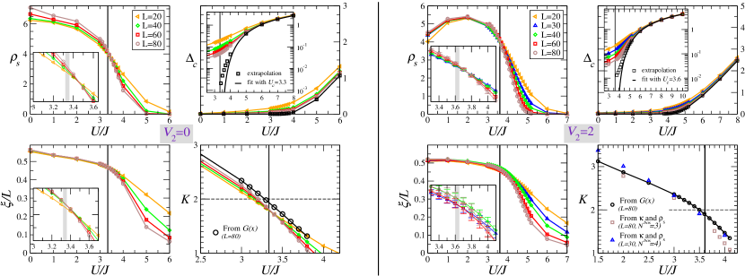
Figure 12: (Color online) Superfluid-Mott insulator transition for $n=1$. Cuts along the $U$-axis for $V_{2}=0$ and 2. Left: data giving similar results to those of Ref. Kuhner2000, (the vertical bar being $U_{c}\simeq 3.33\pm 0.1$). Data are computed with $N^{\text{bos}}=4$ and the Luttinger exponent $K$ is determined using either $\rho_{s}$ and $\kappa$ or $G(x)$ (see Sec. III.1). Scaling of $\rho_{s}$, $\xi/L$ and the criteria $K_{c}=2$ gives the same critical point within error bars. The scaling of the condensate fraction $f_{c}$ (not shown) is not simple at the transition and the HCB scaling $f_{c}\propto\sqrt{N}$ does not hold. Right: the same observables for $V_{2}=2$ and $N^{\text{bos}}=3$ (this cutoff induces a non-physical decrease of the superfluidity at small $U$, but does not affect the transition as seen, for instance, from the behavior of the Luttinger parameter $K$ for $N^{\text{bos}}=4$). Insets show scaling behavior for $\rho_{s}$ and $\xi/L$ after averaging over several different $\phi$. A critical point $U_{c}\simeq 3.6\pm 0.1$ is found which corresponds to $K_{c}\simeq 2$. Furthermore, the one-particle gap (not averaged over $\phi$) is best fitted by a Kosterlitz-Thouless opening (we fixed $U_{c}=3.6$ for the fit). Up to numerical precision, we infer from these results that there is a direct transition between the SF and the MI phases, with no intervening BG phase.

Superfluid–Mott transition and intervening Bose-glass phase – An important question is whether the SF and Mott touch each other at small but finite $V_{2}$. In other words, is there always an intervening BG phase between the SF and the MI phases as for the RBD Prokofev1998 ; Rapsch1999 ? For the bichromatic potential, we however have reasons to think that small $V_{2}$ might not be as relevant as for true disorder since a large critical value exists for both hard-core and free bosons. To address this issue numerically, we have compared the scaling of the most relevant observables for the known case $V_{2}=0$ and for $V_{2}=2$ (see Fig. 12). When $V_{2}=0$, the SF-MI transition is of the Kosterlitz-Thouless type leading to an opening of the one-particle gap $\Delta_{c}\propto\exp(-A/\sqrt{U-U_{c}})$ above the critical value $U_{c}$, with $A$ a constant. Such an opening gives a good fit to the extrapolated data (see Fig. 12) but does not precisely give $U_{c}$. Finding $U_{c}$ is rather achieved by using the weak-coupling RG result $K_{c}=2$ for the KT transition. Fig. 12 shows that $U_{c}\simeq 3.3\pm 0.1$ for $V_{2}=0$ in agreement with results of Ref. Kuhner2000, . Within error bars, the scalings of the superfluid stiffness $\rho_{s}$ and correlation length also agree with this critical point. Note that because of the very slow opening of the one-particle gap in a KT transition, the correlation length and superfluid density show much smoother finite size effects than for the SF–BG transition illustrated in Fig. 10. For $V_{2}=2$, if a BG is present in between the SF and MI phase, the one-particle gap $\Delta_{c}$ should open after the superfluid stiffness scales to zero. Up to numerical accuracy, data are consistent with a direct SF-MI transition of the KT type with a slightly larger critical interaction $U_{c}\simeq 3.6\pm 0.1$. We observed that averaging over $\phi$ is needed to ensure a good crossing of the scaling curves (see insets of Fig. 12). Note that for the RBD situation, $V_{2}=2$ would correspond to a disorder amplitude $\Delta=1$ in Ref. Rapsch1999, (or $\Delta=0.5$ in Ref. Prokofev1998, ) for which the BG phase already has a significant width. Interestingly, the $n=1$ phase diagram has a similar shape as the one with a commensurate potential with $r=1/2$ Rousseau2006 . In this case, there is at large $V_{2}$ a charge density wave phase is a gapped with two particles each two sites for which $K_{c}=1/2$. A direct SF-MI transition is found because the term (7) will not be relevant for small $V_{2}$. Our results suggest that in the incommensurate case, the potential remains irrelevant as well.

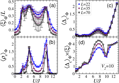
Figure 13: (Color online) Reentrances of the SF phase with increasing interactions. Cut at $V_{2}=10$ in the phase diagram of Fig. 11. Error bars are related to the average over the phase-shift $\phi$ (about twenty samples). The scalings of the correlation length (a) and of the superfluid density (b) suggest two reentrances of the SF phase as $U$ is increased. In between, a localized phase is found and a MI phase is obtained at large $U$ according to the gap (c). In the intermediate BG phase (for $U\simeq 6$–9), a small gap is found, but for the chosen sizes $L=22,35$ and 70, the scaling $\xi\sim 1/\Delta$ shown in (d) seems to be satisfied only in the MI phase, meaning that strong finite size effects are present.

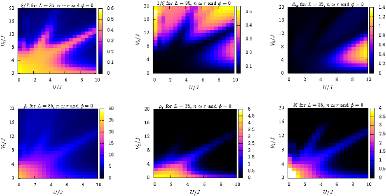
Figure 14: (Color online) Phase diagram for $n\simeq r$. Observables are computed on a system with fixed size $L=35$ and fixed phase-shift $\phi=0$. A large ICDW phase emerges at large $U$. A finite $V_{2}$ is required to stabilize it. The SF phase extends along the $V_{2}=0$ contrary to the phase diagram with $n=1$.

Superfluid–Bose Glass transition – We now turn to the discussion of the contour of the SF-BG transition which displays a “hand print” pattern. First, contrary to the RBD, the BG phase emerges only above $V_{2}^{c}=4$ and for much larger values for small $U$. Secondly, $V_{2}^{c}$ increases with $U$ at small $U$ which is similar to the delocalization by interactions observed in the RBD case. Similarly to what was found in Fig. 10, the inverse correlation length has a power-law behavior above the critical point with a Luttinger parameter smaller than $3/2$. The convexity of the SF phase contours changes contrary to the RBD phase diagram, leading to this hand print pattern. To understand if these reentrances of the SF phase inside the BG phase are not a finite size effect and remain after averaging over $\phi$, we show the averaged $\langle{\rho_{s}}\rangle_{\phi}$ and $\langle{\xi}\rangle_{\phi}$ for various system sizes in Fig. 13. The behavior of $\xi$ and $\rho_{s}$ suggests two reentrances of the SF phase and in particular, a sharp but clear one close to the transition to the MI phase. The $U=V_{2}$ line corresponds to the “transition” between the MI and BG phases in the atomic limit. It gives a rough estimate for the extension of a SF phase at large $U$ and $V_{2}$ which does not occur for the RBD situation. We expect that the SF phase vanishes for large $U$ and that there is a direct MI-BG transition around the $U=V_{2}$ line. A similar emergence of the superfluid phase around the atomic limit was found in Ref. Rousseau2006, for the case of a commensurate potential where the SF phase competes a CDW and a MI phase. In Fig. 13, the intermediate localized phase between the two SF reentrances displays a small gap. This phase could have a finite gap but we observe that if so, it cannot be distinguished from finite size effects. Comparing again with the commensurate case Rousseau2006 , the main difference (apart from the finite gap) is the extension of the SF phase along the $U=0$ line. For the Harper model, there is no such extension because of the localization of the single-particle wave-function.

III.6 Phase diagram close to the density $n=r$

A density which satisfies the criteria $n\simeq r$ allows for the realization of an ICDW phase which competes with the SF and BG phases. The $(U,V_{2})$ map of the observables is given in Fig. 14. The ICDW phase has a finite gap and exponentially decaying correlations as the MI phase. Similar qualitative features are found with the ICDW phase replacing the MI phase. However, a finite $V_{2}$ is of course required to stabilize the ICDW phase contrary to the MI phase. Secondly, a finite $V_{2}$ is needed to stabilize the BG phase. As a consequence, the SF phase extends to large $U$ close to the $V_{2}=0$ line. As discussed in section II, the ICDW is a new feature compared with the RBD phase diagram given in Refs. Prokofev1998, ; Rapsch1999, for $n=0.5$. Similar reentrances of the SF phase into the BG phase are found at fixed $V_{2}$ and increasing $U$. The $U=\infty$ line of the phase diagram would give an ICDW phase everywhere except for $V_{2}=0$ since the $n=r$ plateau occurs as soon as $V_{2}$ is finite in the HCB limit.

III.7 Phase diagram for a generic density $n=1/2$

Lastly, the phase diagram for a generic density $n=1/2$ has been computed to discuss only the competition between the SF and BG phases (data not shown, see phase diagram in Fig. 1 for results). We must note that, ICDW plateaus can however appear for generic density in a region where $U\sim V_{2}$, as we show in Fig. 6 for the particular choice of parameters $V_{2}=8$ and $U=6$. In this case, the ICDW phase would have a finite domain in the $(U,V_{2})$ map (contrary to the $n=r$ phase diagram), because the ICDW phase is not realized in the HCB limit. The observables suggest that $\Delta_{c}$ remains zero in the whole parameter range, while the BG is bounded by the $V_{2}=4$ line and the SF phase slightly extends inside the BG phase for small $U$. However, critical values $V_{2}^{c}$ for the SF-BG transition are found to be smaller than for $n=r$, themselves smaller than for $n=1$. The same qualitative argument stating that the lower the density, the closer the physics is to the HCB can be put forward. The SF region extends with the density of the system. This observation will be now more precisely discussed.

III.8 Delocalization via increasing the density of bosons

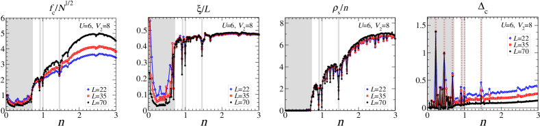
Figure 15: (Color online) Delocalization by increasing the number of particles. Observables for increasing density when $V_{2}\simeq U$ (same parameters as in Fig. 6). There is a delocalization transition with increasing density. A few ICDW phases can be seen at intermediate fillings (dashed brown vertical lines in the r.h.s. figure showing the one=particle gap $\Delta_{c}$). Grey areas denote the localized regions (either BG or ICDW). The weakening of the superfluidity at large density might be an artefact of the cut-off in the number of bosons kept per site which is here $N^{\text{bos}}=4$.

An complementary approach to these $(U,V_{2})$ phase diagrams at fixed density is to keep $U$ and $V_{2}$ constant and to look at the observables as a function of the density $n$. From dipole oscillations measurements, Lye et al. Lye2007 observed a delocalization transition by increasing the number of particles. We now address the non-trivial case of $U\sim V_{2}$ by setting $U=6$ and $V_{2}=8$ corresponding to the parameters of the $n(\mu)$ curve of Fig. 6. Results for the same observables as for the phase diagrams are plotted in Fig. 15. We found transitions between the three different phases BG, ICDW and SF. At low densities, double occupation for bosons is strongly suppressed because of the finite $U$. Consequently, the behavior is qualitatively the one HCB would have: $V_{2}$ being larger than 4, localization exists at low densities. The superfluid density, correlation length and one-particle gap confirm the presence of the BG phase. At large densities, a SF emerges which is something well-known without disorder because the lobes of the Mott phases shrink at large densities Kuhner2000 . In addition, the disordered potential has a tendency to reduce the size of the Mott phases as we have seen. Very qualitatively, some particles fill the wells of the disorder potential so that the remaining ones feel a smoother effective potential allowing for a gain in kinetic energy leading to superfluidity. This behavior for an irrational $r$ is qualitatively similar to what was observed for a rational $r$ (see Fig. 23 of Ref. Rousseau2006, ) except that no BG, but a “weakly superfluid” phase is realized in this latter case. Besides this sharp BG-SF transition, peaks in the one-particle gap $\Delta_{c}$ uncover the presence of ICDW phases within both the BG and the SF phases. These phases naturally correspond to the plateaus in Fig. 6.

IV Probing the Bose-glass phase with out-of-equilibrium dynamics

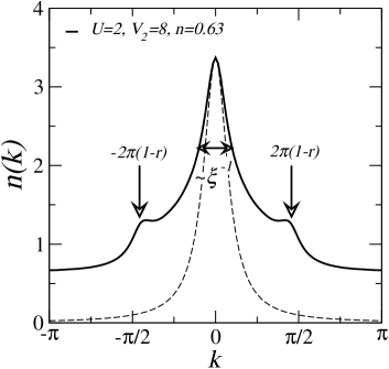
Figure 16: Typical $n(k)$ in the Bose-glass phase of Fig. 10 in a system without a trap. Satellites peaks at wave vector $2\pi(1-r)$ are visible if the disorder is not too strong. The width of the middle peak typically gives the inverse correlation length (a Lorentzian of width $\xi$ computed from Eq. (14) is given in dashed lines for a qualitative comparison).

IV.1 Static observables

The question of probing experimentally the BG phase with respect to the other possible phases is particularly important. First, the simplest observable obtained after time-of-flight measurements is related to the momentum distribution of the atoms $n(k)$. This measure helps distinguish between coherent and incoherent phases by looking, in particular, at the $k=0$ peak. A sharp and high peak is the signature of a coherent phase, the superfluid phase. Because of short-range correlations, both the MI and the BG phases will give a much smaller peak broadened with a typical width of $\xi^{-1}$. Fig. 16 displays $n(k)$ in the BG at small $U$. In addition to the central peak, satellites peaks at $k=\pm 2\pi(1-r)$ emerge as a signature of the underlying superlattice. However, in the experiment pictures, the Wannier envelope and the broadening of the peaks due to scattering events during the time-of-flight will change the observed shape. It is expected that the additional satellite peaks are too small to be experimentally resolved and are washed out if either $V_{2}$ and/or $U$ are too large. Thus, $n(k)$ can only be used to distinguish the superfluid from the Bose-glass or Mott insulating phases. However, it would not help distinguish the MI from the BG phase. Refs. Roth2003, ; Roscilde2007, found a similar behavior and, in the second reference, a non-monotonic evolution of the central peak $n(k=0)$ with increasing $V_{2}$ has been established. The reinforcement of the superfluidity upon increasing $V_{2}$ at fixed $U$ in a trapped cloud must be reminiscent of the MI-SF-BG transitions of the phase diagrams of Fig. 1. Noise correlations Altman2004 were proposed Rey2006 ; Roscilde2007 as a possible probe for the BG phase and measured in Ref. Guarrera2008, . However, this observable catches the fact that density correlations reveal the presence of the underlying superlattice Rey2006 ; Roscilde2007 but not the gapless nature of the excitations Roscilde2007 . It is therefore necessary to look for additional evidence of localization.

IV.2 Expansion in the lattice potential

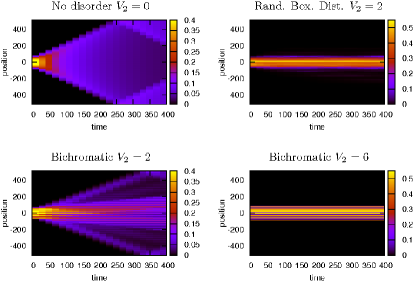
Figure 17: (Color online) Expansion of HCB condensates. At $t=0$, the system is in the ground-state of the hamiltonian with the trap plus “disorder” potentials using a fixed chemical potential $\mu=0$ (about 51 particles) and a trap frequency $\omega=0.03$. At $t>0$, the trap confinement is switched off abruptly. Figures show the evolution of the local density profile as a function of time. An expansion is observed for systems with $V_{2}=0$ (without disorder) and $V_{2}=2$, but not for a random potential and a bichromatic potential with $V_{2}=6>V_{2}^{c}$. For the RBD, $V_{2}$ defines the width of the box distribution. When there is an expansion, reflections on the boundaries of the box in which the condensate expands can be seen.

As often done in experiments Clement2005 ; Fort2005 ; Lye2005 ; Clement2006 ; Clement2008 ; Chen2007 ; Lye2007 , transport measurements are a better fashion to probe localization. In order to show the existence of a critical point for the localization, we propose to look at the expansion of the cloud when the trap is released Rigol2004a ; Fort2005 ; Clement2005 ; Rigol2005 ; Clement2006 ; Clement2008 ; Sanchez-Palencia2007 . Observing the expansion in the optical lattice is a particularly appealing experiment as the hamiltonian governing the dynamics is the one of the bulk system (with $\omega=0$) for which we have computed the equilibrium phase diagram. The confinement is used here to prepare an out-of-equilibrium state for this hamiltonian.

For the sake of clarity, we first discuss the expansion of HCB. The spreading has been studied before in the HCB limit for homogeneous lattices Rigol2005 , and for soft-core bosons in commensurate lattices Rodriguez2006 . Fig. 17 displays the expansion for free HCB ($V_{2}=0$), for two bichromatic potential amplitudes, below ($V_{2}=2$) and above ($V_{2}=6$) the equilibrium critical point, and also a situation with a RBD potential of an amplitude $V_{2}=2$. The system is prepared in the ground-state of the hamiltonian with the confining potential (we chose a trap frequency of $\omega=0.03$). At $t=0$, the trap frequency is set to zero and the condensate is free to expand into the lattice. For $V_{2}=0$, the expansion of the edges of the condensate is roughly linear, with a typical velocity $2J$ corresponding to the maximum group velocity (see below). For the RBD potential, the expansion is inhibited for the amplitude $V_{2}=2$. However, for the bichromatic set-up, the same potential strength does not prevent the condensate from expanding. Still, $V_{2}=6$ induces a localization of the condensate similar to the one observed for the RBD potential.

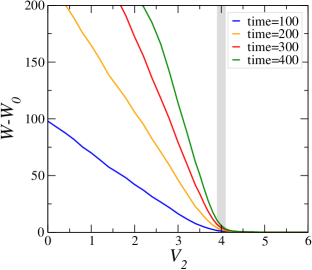
Figure 18: (Color online) Dynamical critical point – Width of the atomic distribution $W=\sqrt{\overline{n_{j}(j-j_{0})^{2}}}$ of a HCB condensate as a function of $V_{2}$ for several increasing times (in units if the hopping). The width $W_{0}$ at $t=0$ has been subtracted for clarity. Parameters are the same as in Fig. 17. Up to finite trap frequency effects (see text), the dynamical critical point is identical to the equilibrium one (at least for HCB).

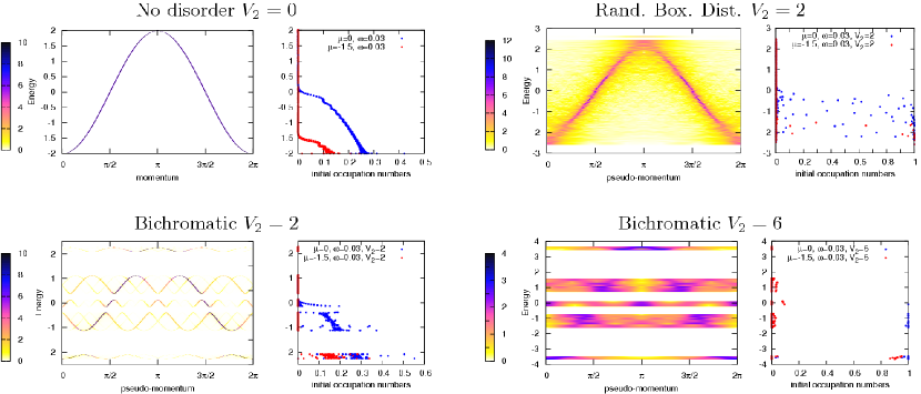
Figure 19: (Color online) Effective dispersion relations for HCB – the Fourier transform of the single-particle wave functions $|{\psi_{k}}|^{2}$ is plotted as a function of the single-particle energy and the pseudo-momentum $k$. At the right each dispersion curve is the initial occupation numbers (from the state prepared using the trap confinement) v.s. the same single-particle energies for two different chemical potential $\mu=-1.5,0$. This shows which states participate to the expansion. Other parameters are the same as for the expansions shown in Fig. 17.

One may ask whether the critical point of the dynamical localization observed in Fig. 17 is the same as the equilibrium one. In the case of HCB, we know that all single-particle wave-functions are localized above $V_{2}=4$ (see Sec. II.1 and references therein). Consequently, we expect the dynamical critical point to be identical to the equilibrium one. To support this statement, we show in Fig. 18 the width of the atomic distribution of the condensate after several times of expansion, as a function of the “disorder strength” $V_{2}$. The dynamical critical point is found to be very close to $V_{2}=4$, within a $\pm 0.1$ window (grey rectangle in Fig. 18). One observes that, slightly above $V_{2}=4$, the condensate still spreads a little bit with time. This may be understood as a finite trap frequency effect. Indeed, the edges of the condensate can spread over a few sites if the initial trap is too steep. In this case, the starting atomic distribution is too far from the local atomic distribution that is expected (locally) in the bulk of a non-trapped system, and particles have to be redistributed. In the limit of vanishing initial trap frequency, we expect the transition to be sharper. Note that, as the localization of all single-particle wave-functions in the spectrum does not depend on $r$ (provided it is irrational), we expect the equality of the dynamical and equilibrium critical points to hold independently of $r$. Fig. 18 may be interpreted as the vanishing of all effective group velocities at the critical point (see below). Thus, the exact critical value $V_{2}^{c}=4$ for the localization could be probed experimentally with this technique for free or hard core bosons.

Following Ref. Diener2001, , a more precise description of the HCB expansion can be carried out by looking at the one-particle effective dispersion $\varepsilon(k)$ for HCB. Without translational symmetry, wave vectors $k$ are not good quantum numbers but looking at the Fourier transform of the one-particle wave functions $\psi_{k}\sim\sum_{j}e^{ikj}\psi_{j}$ and plotting $|{\psi_{k}}|^{2}$ as a function of the pseudo-momentum $k$ provides an effective dispersion. The features of the expansion depend mainly on two properties. First, the group velocities $v_{g}(k)=\partial\varepsilon(k)/\partial k$ derived from the effective dispersion relation convey the typical maximal speed at which expansion evolves. Second, the expansion also strongly depends on the initial occupation numbers $n_{\varepsilon}(t=0)$ of the eigenstates of the hamiltonian with $\omega=0$. This occupation is plotted together with the dispersion relation as a function of the “single-particle energy” $\varepsilon$ in Fig. 19 corresponding to the expansion observed in Fig. 17. For $V_{2}=2$, for which there is no localization, the effective relation dispersion displays gaps as we have seen from section II and well-defined bands with a shorter periodicity originating from the band foldings induced by the potential (see Sec. II). Compared with the single cosine dispersion obtained without disorder, several shifted bands exist due to Bragg scattering with the potential. One can convince oneself that opening gaps lowers the maximum possible group velocity. Thus, compared to a system with no disorder (Fig. 19, $V_{2}=0$), the expansion for the bichromatic potential below $V_{2}=4$ will always be slower if the $\varepsilon=0$ state (associated with the maximum group velocity $2J$) is occupied in the initial state without disorder. This explains the qualitative features of the situations for which the condensate expands in Fig. 17. When $V_{2}=0$, the expansion is slower when the chemical potential is below much 0 (not shown), as can be guessed from the initial occupation numbers in Fig. 19. When $V_{2}=2$, the structure of the expansion is rather homogeneous at low chemical potential (not shown) but becomes inhomogeneous and faster for larger $\mu$ (see Fig. 17). The presence of two different speeds might stem from populating bands with different maximum group velocities as can be seen in Fig. 19. For the bichromatic potential with $V_{2}=6$, no bands can be distinguished as the signal does not show well-defined pseudo-momentums. The RBD potential displays a very different effective dispersion faded by the disorder, but which still retains the whole feature of the cosine dispersion without disorder. These two pictures illustrate that the localization mechanism for the bichromatic and a RBD potential is qualitatively different: the first one is rather associated with a band folding mechanism while the second rather corresponds to strongly scattered single-particle states. In this respect, one can view the “weakly superfluid” phase found for commensurate superlattices with a large $V_{2}$ in Ref. Rousseau2006, as a precursor of the Bose-glass phase of incommensurate lattices.

How these results can carry to investigate the physics at finite $U$ is an important and challenging question that needs further investigations going clearly beyond the goal of this paper. Indeed, from the numerical point of view, the expansion of strongly correlated soft-core bosons is accessible with time-dependent DMRG only until times of order $10J$ Rodriguez2006 , while Fig. 18 shows that a reasonable determination of the out-of-equilibrium critical point requires times of, at least, $100J$. Thus, the question of the dynamical localization at finite $U$ of the model (3) and its relation with the equilibrium phase diagrams of Fig. 1 remains an open question. First, the most naive prediction would be to expect a similar physics than the HCB one to hold, at least for large enough interations. Further qualitative arguments can be given on the expansion for intermediate $U$, for which we can use two results from the equilibrium phase diagrams studied in Sec. III: (i) the critical values to observe localization are all larger than $V_{2}=4$, whatever $U$ or the density, (ii) at small densities, the physics is essentially equivalent to the one of HCB. First consider a situation where $V_{2}\leq 4$. The starting trapped state is expected to have regions which can be locally SF or MI but not BG, since there is no intervening BG phase. Provided $V_{2}\leq 4$, an expansion is then expected systematically (whatever $U$ or the total number of particles), because the edges of the condensate would be in a SF state (see examples of expansions of strongly-correlated soft-core bosons in Ref. Rodriguez2006 ). For $V_{2}>4$, the situation is more subtle as, for a given $U$ and $V_{2}$, the occurence of localization depends on density in the non-trapped condensate (see for instance Fig. 15). The starting state structure is complex and local-density approximation not necessarily valid Roscilde2007 . Very qualitatively, the edges of the condensate would be in a localized state while, if the density at the center of the cloud is large enough, SF or Mott regions could also appear. However, if expansion there is, the local density will decrease with time. When the density becomes small enough to neglect interactions, localization would then be expected since $V_{2}>4$ and one enters the HCB regime. A possible scenario could thus be a systematic localization after either a transient regime with expansion, or no transient regime. However, ascertaining whether the above qualitative arguments could be spoiled by other effects is difficult. For instance, it is known in the completely different limit of very weakly interacting bosons (Gross-Pitaevskii limit) that non-linear effects due to interactions can lead to some kind of localization even in a purely effective periodic potential Trombettoni2001 ; Anker2005 . How to go from such a limit to the relevant one for the Anderson localization in strongly interacting one dimensional systems is clearly a question that will need further experimental and theoretical work.

V Conclusion

The Bose-Hubbard model with a quasi-periodic potential was shown to display a rich phase diagram including a Bose-glass phase (localized but compressible), and incommensurate charge-density wave phases in addition to the superfluid and Mott phases. While localization induced by this random-like potential is found, the underlying mechanism differs from the RBD situation: the band folding mechanism known previously for free and hard-core bosons (or fermions) holds for soft-core bosons, leading to a finite critical value of the localization transition $V_{2}^{c}\geq 4$. The critical values found are high, possibly sufficiently high to allow for an experimental demonstration of a localization transition. In this perspective, static observables give a clear evidence to distinguish between coherent and localized phases, but their ability to sort the BG from the (small-$V_{2}$) MI phase is less obvious. On the contrary, the expansion of the condensate after switching off the confinement is proposed to provide a simple and rather clear signal to detect the localization transition. This was shown explicitly in the case of hard-core bosons but remains an open question for soft-core bosons.

Appendix A Method to fit the bosonic Green’s function on finite systems

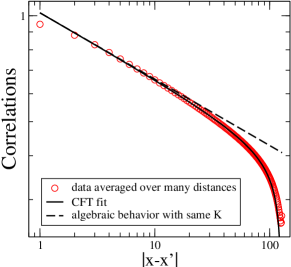
Figure 20: (Color online) A typical example of fitting the averaged data from DMRG with conformal field theory results to extract the Luttinger exponent $K$. System size is $L=128$.

We use conformal field theory results Cazalilla2004 for a system of length $L$ with open boundary conditions to fit the bosonic Green’s function defined in Eq. (13). In the case of correlations of the type $\langle{e^{i\theta(x)}e^{-i\theta(x^{\prime})}}\rangle$ one has :

$$G(x,x^{\prime})=A\left[\frac{\sqrt{d(2x|2L)d(2x^{\prime}|2L)}}{d(x+x^{\prime}|2L)d(x-x^{\prime}|2L)}\right]^{\displaystyle\frac{1}{2K}}\,,$$ (18)

with $K$ the Luttinger parameter, $A$ a constant and $d$ the conformal length

$$d(x|L)=\frac{L}{\pi}\left|\sin\left(\frac{\pi x}{L}\right)\right|\,.$$

Because there is no translational invariance, the correlations depend on both $x$ and $x^{\prime}$. Hence, in order to perform a fit, one has to average Eq. (18) over the results obtained with fixed distance $x^{\prime}-x$. Strictly speaking, formula (18) is valid for $1\ll x,x^{\prime},|{x^{\prime}-x}|\ll L$ and we have to remove the corresponding contributions. Practically, fits are rather good up to distances comparable with $L$ as one can see in Fig. 20 and significantly improves the determination of $K$ compared with a simple algebraic fit.

References

- (1) P. W. Anderson, Phys. Rev. 109, 1492 (1958).
- (2) P. A. Lee and T. V. Ramakrishnan, Rev. Mod. Phys. 57, 287 (1985).
- (3) E. Abrahams, P. W. Anderson, D. C. Licciardello, and T. V. Ramakrishnan, Phys. Rev. Lett. 42, 673 (1979).
- (4) T. Giamarchi and H. J. Schulz, Europhys. Lett. 3, 1287 (1987).
- (5) T. Giamarchi and H. J. Schulz, Phys. Rev. B 37, 325 (1988).
- (6) M. P. A. Fisher, P. B. Weichman, G. Grinstein, and D. S. Fisher, Phys. Rev. B 40, 546 (1989).
- (7) G. G. Batrouni, R. T. Scalettar, and G. T. Zimanyi, Phys. Rev. Lett. 65, 1765 (1990).
- (8) R. T. Scalettar, G. G. Batrouni, and G. T. Zimanyi, Phys. Rev. Lett. 66, 3144 (1991).
- (9) N. V. Prokof’ev and B. V. Svistunov, Phys. Rev. Lett. 80, 4355 (1998).
- (10) S. Rapsch, U. Schollwöck, and W. Zwerger, Europhys. Lett. 46, 559 (1999).
- (11) I. Bloch, J. Dalibard, and W. Zwerger, Rev. Mod. Phys. 80, 885 (2008).
- (12) J. E. Lye, L. Fallani, M. Modugno, D. S. Wiersma, C. Fort, and M. Inguscio, Phys. Rev. Lett. 95, 070401 (2005).
- (13) D. Clément, A. F. Varón, M. Hugbart, J. A. Retter, P. Bouyer, L. Sanchez-Palencia, D. M. Gangardt, G. V. Shlyapnikov, and A. Aspect, Phys. Rev. Lett. 95, 170409 (2005).
- (14) C. Fort, L. Fallani, V. Guarrera, J. E. Lye, M. Modugno, D. S. Wiersma, and M. Inguscio, Phys. Rev. Lett. 95, 170410 (2005).
- (15) T. Schulte, S. Drenkelforth, J. Kruse, W. Ertmer, J. Arlt, K. Sacha, J. Zakrzewski, and M. Lewenstein, Phys. Rev. Lett. 95, 170411 (2005).
- (16) D. Clément, A. F. Varón, J. A. Retter, L. Sanchez-Palencia, A. Aspect, and P. Bouyer, New J. Phys. 8, 165 (2006).
- (17) Y. P. Chen, J. Hitchcock, D. Dries, M. Junker, C. Welford, and R. G. Hulet, Phys. Rev. A 77, 033632 (2008).
- (18) D. Clément, P. Bouyer, A. Aspect, and L. Sanchez-Palencia, Phys. Rev. A 77, 033631 (2008).
- (19) B. Paredes, F. Verstraete, and J. I. Cirac, Phys. Rev. Lett. 95, 140501 (2005).
- (20) U. Gavish and Y. Castin, Phys. Rev. Lett. 95, 020401 (2005).
- (21) R. B. Diener, G. A. Georgakis, J. Zhong, M. Raizen, and Q. Niu, Phys. Rev. A 64, 033416 (2001).
- (22) B. Damski, J. Zakrzewski, L. Santos, P. Zoller, and M. Lewenstein, Phys. Rev. Lett. 91, 080403 (2003).
- (23) J. E. Lye, L. Fallani, C. Fort, V. Guarrera, M. Modugno, D. S. Wiersma, and M. Inguscio, Phys. Rev. A 75, 061603(R) (2007).
- (24) L. Fallani, J. E. Lye, V. Guarrera, C. Fort, and M. Inguscio, Phys. Rev. Lett. 98, 130404 (2007).
- (25) V. Guarrera, L. Fallani, J. E. Lye, C. Fort, and M. Inguscio, New J. Phys. 9, 107 (2007).
- (26) V. Guarrera, N. Fabbri, L. Fallani, C. Fort, K. M. R. van der Stam, and M. Inguscio, arXiv:0803.2015.
- (27) S. Aubry and G. André, Ann. Israel Phys. Soc 3, 133 (1980).
- (28) B. Simon, Adv. Appl. Math 3, 463 (1982); J. B. Sokoloff, Phys. Rep. 126, 189 (1985); H. Hiramoto and M. Kohmoto, Int. J. of Mod. Phys. B 6, 281 (1992).
- (29) D. J. Thouless, Phys. Rev. B 28, 4272 (1983).
- (30) M. Kohmoto, L. P. Kadanoff, and C. Tang, Phys. Rev. Lett. 50, 1870 (1983).
- (31) M. Kohmoto, Phys. Rev. Lett. 51, 1198 (1983); C. Tang and M. Kohmoto, Phys. Rev. B 34, 2041 (1986).
- (32) J. X. Zhong and R. Mosseri, J. Phys.: Cond. Matt. 7, 8383 (1995); F. Piéchon, Phys. Rev. Lett. 76, 4372 (1996).
- (33) J. Vidal, D. Mouhanna, and T. Giamarchi, Phys. Rev. Lett. 83, 3908 (1999); Phys. Rev. B 65, 014201 (2001).
- (34) R. Roth and K. Burnett, Phys. Rev. A 68, 023604 (2003).
- (35) N. Bar-Gill, R. Pugatch, E. Rowen, N. Katz, and N. Davidson, arXiv:cond-mat/0603513.
- (36) P. J. Y. Louis and M. Tsubota, arXiv:cond-mat/0609195.
- (37) P. Buonsante and A. Vezzani, Phys. Rev. A 70, 033608 (2004).
- (38) P. Buonsante, V. Penna, and A. Vezzani, Phys. Rev. A 72, 031602(R) (2005).
- (39) V. G. Rousseau, D. P. Arovas, M. Rigol, F. Hébert, G. G. Batrouni, and R. T. Scalettar, Phys. Rev. B 73, 174516 (2006).
- (40) T. Roscilde, Phys. Rev. A 77, 063605 (2008).
- (41) http://en.wikipedia.org/wiki/Continued_fraction.
- (42) F. D. M. Haldane, Phys. Rev. Lett. 47, 1840 (1981).
- (43) M. A. Cazalilla, J. Phys. B 37, S1 (2004).
- (44) T. Giamarchi, Quantum Physics in one Dimension International series of monographs on physics Vol. 121 (Oxford University Press, Oxford, UK, 2004).
- (45) G. I. Dzhaparidze and A. A. Nersesyan, JETP Lett. 27, 334 (1978); V. L. Pokrovsky and A. L. Talapov, Phys. Rev. Lett. 42, 65 (1979); H. J. Schulz, Phys. Rev. B 22, 5274 (1980).
- (46) J. M. Kosterlitz and D. J. D J Thouless, J. Phys. C: Solid State Phys. 6, 1181 (1973); J. M. Kosterlitz, J. Phys. C: Solid State Phys. 7, 1046 (1974); V. L. Berezinskii, Sov. Phys. JETP 32, 493 (1971).
- (47) T. Giamarchi, Physica B 230, 975 (1997).
- (48) T. D. Kühner, S. R. White, and H. Monien, Phys. Rev. B 61, 12474 (2000).
- (49) M. Arlego, D. C. Cabra, and M. D. Grynberg, Phys. Rev. B 64, 134419 (2001).
- (50) M. Rigol and A. Muramatsu, Mod. Phys. Lett. B 19, 861 (2005).
- (51) S. R. White, Phys. Rev. Lett. 69, 2863 (1992).
- (52) S. R. White, Phys. Rev. B 48, 10345 (1993).
- (53) U. Schollwöck, Rev. Mod. Phys. 77, 259 (2005).
- (54) P. Schmitteckert, T. Schulze, C. Schuster, P. Schwab, and U. Eckern, Phys. Rev. Lett. 80, 560 (1998).
- (55) K. Hida, Phys. Rev. Lett. 86, 1331 (2001).
- (56) C. Schuster, R. A. Römer, and M. Schreiber, Phys. Rev. B 65, 115114 (2002).
- (57) I. P. McCulloch, J. Stat. Mech.: Theor. Exp. , P10014 (2007).
- (58) D. Barache and J. M. Luck, Phys. Rev. B 49, 15004 (1994).
- (59) C. Kollath, U. Schollwöck, J. von Delft, and W. Zwerger, Phys. Rev. A 69, 031601(R) (2004).
- (60) E. Altman, E. Demler, and M. D. Lukin, Phys. Rev. A 70, 013603 (2004).
- (61) A. M. Rey, I. I. Satija, and C. W. Clark, Phys. Rev. A 73, 063610 (2006).
- (62) M. Rigol and A. Muramatsu, Phys. Rev. Lett. 93, 230404 (2004).
- (63) L. Sanchez-Palencia, D. Clément, P. Lugan, P. Bouyer, G. V. Shlyapnikov, and A. Aspect, Phys. Rev. Lett. 98, 210401 (2007); B. Shapiro, Phys. Rev. Lett. 99, 060602 (2007).
- (64) K. Rodriguez, S. R. Manmana, M. Rigol, R. M. Noack, and A. Muramatsu, New J. Phys. 8, 169 (2006).
- (65) A. Trombettoni and A. Smerzi, Phys. Rev. Lett 86, 2353 (2001).
- (66) Th. Anker, M. Albiez, R. Gati, S. Hunsmann, B. Eiermann, A. Trombettoni, and M. K. Oberthaler, Phys. Rev. Lett 94, 020403 (2005).