Wide-field Fourier transform spectral imaging

Abstract

We report experimental results of parallel measurement of spectral components of the light. The temporal fluctuations of an optical field mixed with a separate reference are recorded with a high throughput complementary metal oxide semi-conductor camera (1 Megapixel at 2 kHz framerate). A numerical Fourier transform of the time-domain recording enables wide-field coherent spectral imaging. Qualitative comparisons with frequency-domain wide-field laser Doppler imaging are provided.

Many coherent spectral detection schemes using a single detector (or balanced detection) to detect temporal fluctuation spectra in an optical mixing configuration rely on Fourier Transform spectroscopy (FTS) for signal measurement Pike (1970); Chung et al. (1997). They provide a high spectral resolution and shot-noise sensitivity. They allow to shift away the $1/f$ noise of laser intensity fluctuations since the measurement is done with GHz-bandwidth detectors. Most imaging configurations require a spatial scanning of the beam, but two approaches to parallel coherent spectral imaging with a solid-state array detector were presented recently : full-field laser Doppler imaging (LDI) Serov et al. (2002); Serov and Lasser (2005); Serov et al. (2005) and frequency-domain wide-field LDI (FDLDI) Atlan et al. (2006); Atlan and Gross (2006, 2007). In the former approach, the temporal fluctuations of an optical object field impinging on a complementary metal oxide semi-conductor (CMOS) camera are recorded. Spectral imaging is done by calculating the intensity-fluctuation spectrum by a Fourier transform (FT). One major weakness of this approach lies in its inapplicability in low-light conditions. The latter approach uses a spatiotemporal heterodyne detection, which consists in recording an optical mix of the object field with an angularly tilted and frequency-shifted local oscillator (LO). It enables to measure spectral maps with a high sensitivity but requires to acquire the spectral components sequentially by sweeping the LO frequency. We present an alternative approach, designed to combine the advantages of both methods. It uses the properties of digital off-axis holography and FTS to enable exploring of the temporal frequency spectrum of the object field. Basically, the parallel spectral imaging instrument presented here uses a CMOS camera to record the intensity fluctuations of an object field mixed with a separate reference (LO); the field spectral components are calculated by FTS.

The experimental setup is based on an optical interferometer sketched in Fig.1. A CW, 80 mW, $\lambda=$ 658 nm diode (Mitsubishi ML120G21) provides the main laser beam (field $E_{\mathrm{L}}$, angular frequency $\omega_{\mathrm{L}}$). A small part of this beam is split by a prism to form a reference (LO) beam, while the remaining part is expanded and illuminates an object in reflection with an average incidence angle $\alpha\approx 45^{\circ}$. The object is made of a USAF 1951 target set in front of a 4 mm-thick transparent tank, filled with a non dilute intralipid (TM) 10% emulsion. To benefit from heterodyne gain, the field scattered by the object, $E$, is mixed with the LO field $E_{\mathrm{LO}}$ ( $|E_{\mathrm{LO}}|^{2}/|E|^{2}\sim 10^{3})$, and is detected by a CMOS camera (LaVision HighSpeedStar 4, 10 bit, 1024 $\times$ 1024 pixels at $\omega_{\mathrm{S}}/(2\pi)$ = 2.0 kHz frame rate, pixel area ${d_{pix}}^{2}$ with $d_{pix}=17.5~{}\mu\rm m$, set at a distance $d$ = 50 cm from the object. A 10 mm focal length lens is placed in the reference arm in order to create an off-axis ($\theta\approx 1^{\circ}$ tilt angle) virtual point source in the object plane. This configuration constitutes a lensless Fourier holographic setup Stroke (1965).

Figure 1: Setup. LD : single mode laser diode. $M$ : mirror. BE : beam expander. BS : beam splitter. $E$ : object field. $E_{\mathrm{LO}}$ : local oscillator field.

In the detector plane, the LO and object fields are:

$$E_{\mathrm{LO}}(t)={\cal E}_{LO}e^{i\omega_{\mathrm{L}}t}+\textrm{c.c.}$$

$$E(x,y,t)={\cal E}(x,y,t)e^{i\omega_{\mathrm{L}}t}+\textrm{c.c.}$$ (1)

where ${\rm c.c.}$ is the complex conjugate term. The LO beam is a spherical wave propagating along $z$, and thus the LO field envelope ${\cal E}_{LO}$ does not depend on $x,y,t$. The object field envelope ${\cal E}$, which contains information on the object shape, and which may exhibit speckle, depends on position $x,y$. It also depends on time $t$ because of dynamic scattering. The intensity $I$ recorded by the camera can be expressed as a function of the complex fields :

$$I(x,y,t)=\overline{\left|E(x,y,t)+E_{\mathrm{LO}}(t)\right|^{2}}$$ (2)

$$=|{\cal E}(x,y,t)|^{2}+|{\cal E}_{LO}|^{2}$$

$$+{\cal E}(x,y,t){\cal E}^{*}_{LO}+{\cal E}^{*}(x,y,t){\cal E}_{LO}$$

where $\overline{A}$ is the time average of $A$ over the optical period.

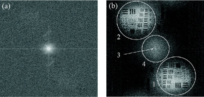
Figure 2: Lensless off-axis holograms reconstructed in the target plane. Images represent the field intensity, displayed in arbitrary logarithmic scale. (a) image obtained from a single hologram. (b) image obtained from the difference of two holograms.

The camera records the interference pattern of the LO field ${\cal E}_{LO}$ with the signal field $\cal E$, the recorded signal $I(x,y,t)$ is the numerical hologram of the object that can be used to reconstruct the object image Schnars and Juptner (1994). Because of the lensless Fourier holographic configuration, the reconstructed image field amplitude $\widetilde{\cal E}$ is obtained from $I$ by a two-dimensional (2D) FT Wagner et al. (1999); Schnars and Juptner (2002); Kreis (2002):

$$\widetilde{\cal E}(k_{x},k_{y})=\textrm{FT}^{2D}~{}I(x,y)$$ (3)

Fig.2 shows intensity images of the USAF target (i.e.$|~{}\widetilde{\cal E}(k_{x},k_{y})|^{2}$) displayed in logarithmic scale (arbitrary units). Fig.2a is obtained from a single frame $I(t_{1})$ recorded at time $t_{1}$. The USAF target is not visible because the noise is too large. To lower the noise, we have recorded two frames $I(t_{1})$ and $I(t_{2})$ at instants $t_{1}$ and $t_{2}$, and substracted them. By making the difference of the two holograms, the noise components which do not vary with time (like the LO beam noise and the CMOS dark signal noise) cancel-out, whereas the Eq.2 holographic cross terms (${\cal E}{\cal E}^{*}_{LO}$ and ${\cal E}^{*}{\cal E}_{LO}$) do not vanish, because the signal field envelopes ${\cal E}(t_{1})$ and ${\cal E}(t_{2})$ are (at least partially) decorrelated in both amplitude and phase from one frame to another as a consequence of dynamic backscattering by the intralipid emulsion. Fig.2b shows the reconstructed intensity image ($|\widetilde{\cal E}^{\prime}|^{2}$) obtained from the difference of two frames. One can notice that the last 4 terms of Eq.2 are visible on Fig.2b. The true image (white circle 1) corresponds to the cross term ${\cal E}{\cal E}^{*}_{LO}$, while the twin image (white circle 2) corresponds to ${\cal E}^{*}{\cal E}_{LO}$. Because of the lensless configuration, the true and twin images are on focus in the same reconstruction plane (i.e. the reciprocal plane of the detector). To prevent overlapping of the true, twin and zero order images in the off-axis holographic configuration, the true image size (circle 1 of diameter 0.75 cm 409 pixels) is $\sim 2.5\times$ smaller than the total 1024 pixels field corresponding to $\lambda d/d_{pix}=1.87$ cm Schnars and Juptner (1994). This means that, on average, one speckle grain is about 2.5 pixels. The light collection efficiency is $2.5^{2}\simeq 6\times$ lower than with on-axis (or inline) holography or with homodyne detection (for which one speckle = 1 pixel). $|{\cal E}_{LO}|^{2}$ contributes to the zero order image Schnars and Juptner (1994); Cuche et al. (2000). It yields the very bright region in the center (null spatial frequency) of Fig.2a and Fig.2b (arrow 3). Contrarily to $|{\cal E}_{LO}|^{2}$, the $|{\cal E}|^{2}$ term is not flat-field. It yields the broad spot in the center of Fig.2b (circle 4). Because the brownian spectrum is narrower than the Nyquist frequency of the time-domain sampling, $\cal E$ and $I$ vary not too fast in time to be sampled properly. It is then possible to record with the CMOS camera the time evolution of intensity fluctuations in time. From a sequence of CMOS images, one can thus extract the Fourier temporal frequency components of the holographic signal, and reconstruct images from these spectral components.

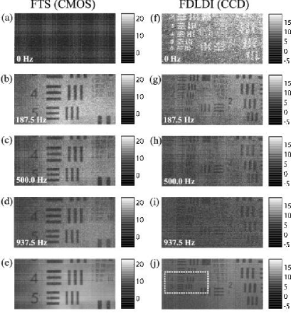
Figure 3: $128\times 256$ pixels images of temporal frequency components of the object field, measured with the presented FTS instrument using a CMOS detector: (a) to (d), and the wide field FDLDI setup using a CCD detector: (f) to (i). (e) and (j): average over frequencies. Color axis is in logarithmic arbitrary units.

We have recorded a data cube made of a sequence of $N$ = 2048 images at a framerate $\omega_{\mathrm{S}}/(2\pi)$ = 2 kHz. A 3D numerical FT (2D for space, 1D for time) was applied to this data to calculate spectral component maps of the object field envelope in the target plane :

$$\widetilde{\widetilde{\cal E}}(k_{x},k_{y},\omega)=\textrm{FT}^{1D}~{}\widetilde{\cal E}(k_{x},k_{y},t)=\textrm{FT}^{3D}~{}{I}(x,y,t)$$ (4)

The FT along the temporal dimension is used to calculate spectral maps of the object field in quadrature (amplitude and phase), and the FT in the spatial dimensions yields the field distribution in the object plane (image). Since we have performed a discrete FT, the 2048 frequency points $\omega$ are linearly spaced between the Nyquist frequencies $\pm 1.0~{}\rm kHz$. The measurement time of the $1024\times 1024\times 2048$ data cube is $\simeq 1$ s, and the $\textrm{FT}^{\textrm{3D}}$ calculation time on a personal computer is about 1 hour nowadays. Fig.3(a) to 3(d) show the images of the object field intensity $|\widetilde{\widetilde{\cal E}}|^{2}$ in the target plane for the frequency components $\omega/(2\pi)=0$ (a), 187.5 (b), 500.0 (c) and 937.5 Hz (d) ($128\times 256$ pixels crops of the total hologram, displayed in logarithmic scale). For $\omega=0$ (a), the LO beam noise is dominant and the target is not visible. For $\omega\neq 0$, the USAF target is visible but the brightness and SNR of the image will decrease with frequency ((b) to (d)). Fig.3(e) shows the image obtained by averaging over all frequencies. We have compared these results with wide-field FDLDI images Atlan et al. (2006); Atlan and Gross (2006) obtained with a charge-coupled device (CCD) camera (PCO Pixelfly: $1280\times 1024$ pixels, framerate: 8 Hz) with four-phase demodulation over 32 images per spectral point, in the same experiment. Fig.3 shows the $128\times 256$ pixels FDLDI images at 0 (f), 187.5 (g), 500.0 (h) and 937.5 Hz (i), while image (j) corresponds to the average over all frequencies. The USAF target is seen on all the images. For $\omega=0$, the target appears as a contrast-reversed image Atlan et al. (2006). Since the pixel size of the CCD camera ($6.7\times 6.7~{}\mu\rm m$) is smaller than its CMOS counterpart ($17.5\mu{\rm m}\times 17.5\mu{\rm m}$), the extension of FDLDI image is larger (the acceptance angle of the receiver is proportional to the inverse of the pixel size). The white dashed rectangle of Fig.3j corresponds to the CMOS-imager field of view. Although the number of recorded spectral points was kept low for the FDLDI measurement compared to the FTS scheme (64 vs. 2048), the total measurement time was much greater (256 seconds vs. 1 second). This difference is due to the throughput discrepancy between the CCD (1.3 Mpixel @ 8 Hz) and the CMOS (1.0 Mpixel @ 2 kHz) receivers.

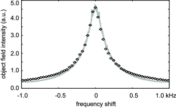
Figure 4: Spectrum of the field dynamically backscattered by a non dilute suspension of intralipid 10% obtained by averaging the object field intensity over 50 $\times$ 50 pixels. FTS (solid gray curve) and FDLDI (points) spectra. Horizontal axis is the frequency $\omega/(2\pi)$ in kHz, vertical axis is signal in linear arbitrary units.

We have computed the frequency spectrum of the light diffused by the intralipid emulsion with FTS. This spectrum is obtained by averaging the object field intensity over a $50\times 50$ pixels region of the reconstructed image. The lineshape is plotted on Fig.4 as a solid gray curve. We have compared its shape with the one obtained with the FDLDI technique (Fig.4 points). The agreement is good except in the tails of the spectrum. The FTS frequency response is imperfectly flat, because of the CCD finite exposure time ($1/\omega_{S}$) that yields signal low pass filtering Picart et al. (2003); Atlan et al. (2007). Moreover, because the signal temporal evolution is sampled at 2 kHz, temporal sampling aliases and spectrum overlap are expected around the Nyquist frequencies $\pm 1$ kHz.

In this Letter, we have shown that the spatiotemporal heterodyne detection recently introduced Atlan and Gross (2006); Atlan et al. (2006); Atlan and Gross (2007) can be adapted to a wide-field Fourier transform spectral imaging scheme with a high throughput array detector. By using an off-axis optical mixing configuration, the object-LO fields cross terms are shifted away from center of the detector reciprocal plane (k-space), contrarily to the object and LO self-beating contributions, which remain unshifted. It is then possible to reject the local oscillator and the object field self-beating contributions accounting for noise. The heterodyne gain provided by optical amplification of the object field by the LO field is essential for a high frame rate camera measurement in low-light conditions, since the object field intensity decreases with the camera exposure time. The ability to filter-off the LO beam noise, yields an optimal sensitivity of 1 photoelectron of noise per pixel. This limit has been reached with 4-phase detection Gross and Atlan (2007), which consists of a discrete Fourier transform on 4 data points to calculate a single frequency component of the object field. Here, the expected noise limit is the same for each frequency component of the object field obtained by discrete Fourier transform. This method might find applications in dynamic light scattering analysis of colloidal suspensions and microfluidic systems.

References

- Pike (1970) E. Pike, Review of Physics in Technology 1, 180 (1970).
- Chung et al. (1997) D. Chung, K. Lee, and E. Mazur, Applied physics. B, Lasers and optics 64, 1 (1997).
- Serov et al. (2002) A. Serov, W. Steenbergen, and F. de Mul, Optics Letters 27, 300 (2002).
- Serov and Lasser (2005) A. Serov and T. Lasser, Opt. Express 13, 6416 (2005).
- Serov et al. (2005) A. Serov, B. Steinacher, and T. Lasser, Opt. Ex. 13, 3681 (2005).
- Atlan et al. (2006) M. Atlan, M. Gross, T. Vitalis, A. Rancillac, B. C. Forget, and A. K. Dunn, Optics Letters 31 (2006).
- Atlan and Gross (2006) M. Atlan and M. Gross, Review of Scientific Instruments 77, 1161031 (2006).
- Atlan and Gross (2007) M. Atlan and M. Gross, Journal of the Optical Society of America A 24, 2701 (2007).
- Stroke (1965) G. W. Stroke, Applied Physics Letters 6, 201 (1965).
- Schnars and Juptner (1994) U. Schnars and W. Juptner, Appl. Opt. 33, 179 (1994).
- Wagner et al. (1999) C. Wagner, S. Seebacher, W. Osten, and W. Juptner, Applied Optics 38, 4812 (1999).
- Schnars and Juptner (2002) U. Schnars and W. P. O. Juptner, Meas. Sci. Technol. 13, R85 (2002).
- Kreis (2002) T. M. Kreis, Optical Engineering 41, 771 (2002).
- Cuche et al. (2000) E. Cuche, P. Marquet, and C. Depeursinge, Applied Optics 39, 4070 (2000).
- Picart et al. (2003) P. Picart, J. Leval, D. Mounier, and S. Gougeon, Opt. Lett. 28, 1900 (2003).
- Atlan et al. (2007) M. Atlan, M. Gross, and E. Absil, Optics Letters 32, 1456 (2007).
- Gross and Atlan (2007) M. Gross and M. Atlan, Optics Letters 32, 909 (2007).