A new dipole-free sum-over-states expression for the second hyperpolarizability

Abstract

The generalized Thomas-Kuhn sum rules are used to eliminate the explicit dependence on dipolar terms in the traditional sum-over-states (SOS) expression for the second hyperpolarizability to derive a new, yet equivalent, SOS expression. This new dipole-free expression may be better suited to study the second hyperpolarizability of non-dipolar systems such as quadrupolar, octupolar, and dodecapolar structures. The two expressions lead to the same fundamental limits of the off-resonance second hyperpolarizability; and when applied to a particle in a box and a clipped harmonic oscillator, have the same frequency-dependence. We propose that the new dipole-free equation, when used in conjunction with the standard SOS expression, can be used to develop a three-state model of the dispersion of the third-order susceptibility that can be applied to molecules in cases where normally many more states would have been required. Furthermore, a comparison between the two expressions can be used as a convergence test of molecular orbital calculations when applied to the second hyperpolarizability.

I Introduction

The sum-over-states (SOS) expressions have been used for more than three decades in the study of nonlinear optical phenomena, and are perhaps the most universally used equations in molecular nonlinear optics. The sum-over-states expression is obtained from quantum perturbation theory and is usually expressed in terms of the matrix elements of the dipole operator, $-ex_{nm}$, and the zero-field energy eigenvalues, $E_{n}$.Boyd ; OrrWard ; KuzBook

The SOS expressions for the first and second hyperpolarizability derived by Orr and Ward using the method of averagesOrrWard are often used because they explicitly eliminate the unphysical secular terms that are present in other derivations.Boyd These secular-free expressions contain summations over all excited states.

Finite-state approximations are used to apply the theory to experimental results. Oudar and Chemla studied the first hyperpolarizability of nitroanilines by considering only two states, the ground and the dominant excited state.OudarChemla Although the general validity of this “two-level” model has been questioned, especially in its use for extrapolating measurement results to zero frequency, the approximation is still widely used in experimental studies of the nonlinear properties of organic molecules.

Several approaches have been used to develop approximate expressions for the second-hyperpolarizability in the off-resonance regime.kuzdirkfirst ; Nakano ; Meyers While such approximations are helpful, they systematically ignore some of the contributions to the SOS expression. As our goal is to derive a general expression that is equivalent to the traditional SOS one, we choose not to make any assumptions a priori about what type of contributions dominate the response. Furthermore, including all the possible contribution is necessary to properly describe the on-resonance behavior, even when only few states contribute to the response.TPAmine

In 2005, Kuzyk used the generalized Thomas-Kuhn sum rules to relate the matrix elements and energies involved in the general Orr and Ward SOS expression for the first hyperpolarizability, and introduced a new and compact SOS expression that does not depend explicitly on dipolar terms.KuzykNew Since the Thomas-Kuhn sum rules are a direct and exact consequence of the Schrödinger equation when the Hamiltonian can be expressed as $H=p^{2}/2m+V(r)$, it follows that the new SOS expression is as general as the original, converges to the same results, and by virtue of its compactness may be more appropriate for the analysis of certain nonlinear optical properties.Fundamental Indeed, Champagne and Kirtman used a comparison between the dipole-free and standard SOS expressions to study the convergence of molecular-orbital calculations.champ In this work, we use the same principle to derive a compact and general dipole-free expression for the second hyperpolarizability.

II Theory

While our method can be applied to non-diagonal components of the second hyperpolarizability, for simplicity we will focus on the diagonal component. The SOS expression for the diagonal term of the second hyperpolarizability $\gamma$ as derived by Orr and Ward in 1971 is given by:OrrWard

$$\gamma_{xxxx}(-\omega_{\sigma};\omega_{1},\omega_{2},\omega_{3})=e^{4}\left({\sum_{lmn}^{\infty}}^{\prime}\frac{x_{0l}\bar{x}_{lm}\bar{x}_{mn}x_{n0}}{D^{-1}_{lmn}(\omega_{1},\omega_{2},\omega_{3})}-{\sum_{mn}^{\infty}}^{\prime}\frac{x_{0m}x_{m0}x_{0n}x_{n0}}{D^{-1}_{mn}(\omega_{1},\omega_{2},\omega_{3})}\right),$$ (1)

where $e$ is the magnitude of the electron charge, $x_{nm}$ the $n,m$ matrix element of the position operator and $h\omega_{i}$ ($i=1,2,3$) are the frequencies of the photons with $\omega_{\sigma}=\omega_{1}+\omega_{2}+\omega_{3}$. The bar operator is defined as:

$$\bar{x}_{nm}=\left\{\begin{array}[]{cc}\Delta x_{n0}\equiv x_{nn}-x_{00}&\mbox{if $n=m$}.\\ x_{nm}&\mbox{if $n\neq m$}\end{array}.\right.$$ (2)

The dispersion of $\gamma$ is given by $D^{-1}_{lmn}(\omega_{1},\omega_{2},\omega_{3})$ and $D^{-1}_{mn}(\omega_{1},\omega_{2},\omega_{3})$ which are defined as follows:

$$D_{lmn}(\omega_{1},\omega_{2},\omega_{3})=\frac{1}{6}\times$$

$$\left\{\frac{1}{(\hbar\Omega_{lg}-\hbar\omega_{\sigma})(\hbar\Omega_{mg}-\hbar\omega_{1}-\hbar\omega_{2})(\hbar\Omega_{ng}-\hbar\omega_{1})}\right.$$

$$+\frac{1}{(\hbar\Omega^{*}_{lg}+\hbar\omega_{3})(\hbar\Omega_{mg}-\hbar\omega_{1}-\hbar\omega_{2})(\hbar\Omega_{ng}-\hbar\omega_{1})}$$

$$+\frac{1}{(\hbar\Omega^{*}_{lg}+\hbar\omega_{1})(\hbar\Omega^{*}_{mg}+\hbar\omega_{1}+\hbar\omega_{2})(\hbar\Omega_{ng}-\hbar\omega_{3})}$$

$$+\frac{1}{(\hbar\Omega^{*}_{lg}+\hbar\omega_{1})(\hbar\Omega^{*}_{mg}+\hbar\omega_{1}+\hbar\omega_{2})(\hbar\Omega^{*}_{ng}+\hbar\omega_{\sigma})}$$

$$+\left.\mbox{all six permutations of $(\omega_{1},\omega_{2},\omega_{3})$ for the above terms}\right\}.$$

(3)

$$D_{mn}(\omega_{1},\omega_{2},\omega_{3})=\frac{1}{6}\times$$

$$\left\{\frac{1}{(\hbar\Omega_{mg}-\hbar\omega_{\sigma})(\hbar\Omega_{mg}-\hbar\omega_{3})(\hbar\Omega_{ng}-\hbar\omega_{1})}\right.$$

$$+\frac{1}{(\hbar\Omega_{mg}-\hbar\omega_{3})(\hbar\Omega^{*}_{ng}+\hbar\omega_{2})(\hbar\Omega_{ng}-\hbar\omega_{1})}$$

$$+\frac{1}{(\hbar\Omega^{*}_{mg}+\hbar\omega_{\sigma})(\hbar\Omega^{*}_{mg}+\hbar\omega_{3})(\hbar\Omega^{*}_{ng}+\hbar\omega_{1})}$$

$$+\frac{1}{(\hbar\Omega^{*}_{mg}+\hbar\omega_{3})(\hbar\Omega_{ng}-\hbar\omega_{2})(\hbar\Omega^{*}_{ng}+\hbar\omega_{1})}$$

$$+\left.\mbox{all six permutations of $(\omega_{1},\omega_{2},\omega_{3})$ for the above terms}\right\},$$

(4)

where spontaneous decay is introduced by defining complex energies:

$$\hbar\Omega_{n}=E_{n0}-i\Gamma_{n},$$ (5)

where $E_{n0}$ is the energy different between the $n^{th}$ excited state and the ground state, and $\frac{\Gamma_{n}}{\hbar}$ is the inverse radiative lifetime of the $n^{th}$ state.

II.1 Dipole-free expression for the second hyperpolarizability

To obtain a dipole-free expression for the second hyperpolarizability we begin by separating explicitly dipolar terms from dipole-free terms in the first term of Eq. 1,

$${\sum_{n}^{\infty}}^{\prime}\left({\sum_{m}^{\infty}}^{\prime}\left({\sum_{l}^{\infty}}^{\prime}\frac{x_{0l}\bar{x}_{lm}\bar{x}_{mn}x_{n0}}{D_{lmn}^{-1}}\right)\right) =$$

$${\sum_{n}^{\infty}}^{\prime}\frac{(\Delta x_{n0}x_{0n})^{2}}{D^{-1}_{nnn}}+{\sum_{n}^{\infty}}^{\prime}{\sum_{m\neq n}^{\infty}}^{\prime}\frac{\Delta x_{m0}x_{0m}x_{mn}x_{n0}}{D_{mmn}^{-1}} + {\sum_{n}^{\infty}}^{\prime}{\sum_{l\neq n}^{\infty}}^{\prime}\frac{\Delta x_{n0}x_{0l}x_{ln}x_{n0}}{D_{lnn}^{-1}}+{\sum_{n}^{\infty}}^{\prime}{\sum_{m\neq n}^{\infty}}^{\prime}{\sum_{l\neq m}^{\infty}}^{\prime}\frac{x_{0l}x_{lm}x_{mn}x_{n0}}{D_{lmn}^{-1}}.$$

The second term in Eq. 1 is already dipole-free.

It should be noted that for non-dipolar systems (such as octupolar chromophores), with $\Delta x_{m0}=0$, only the last term in Eq. LABEL:eq:gsplit contributes to the second hyperpolarizability. The generalized Thomas-Kuhn sum rules can be used to obtain a relationship between the explicitly dipolar terms in terms of only non-dipolar terms:KuzykNew

$$|x_{k0}|^{2}\Delta x_{k0}=-{\sum_{n\neq k}}^{\prime}\frac{(E_{nk}+E_{n0})}{E_{k0}}x_{0k}x_{kn}x_{n0}.$$ (7)

We stress that the only assumption made in the derivation of Eq. 7 is that the sum rules hold, which is the case when the unperturbed Hamiltonian describing the system is conservative.

Substituting Eq. 7 into Eqs. LABEL:eq:gsplit and 1 yields the dipole-free expression for the second hyperpolarizability:

$$\gamma_{xxxx}(-\omega_{\sigma};\omega_{1},\omega_{2},\omega_{3})=e^{4}{\sum_{n}^{\infty}}^{\prime}{\sum_{m\neq n}^{\infty}}^{\prime}{\sum_{l\neq n}^{\infty}}^{\prime}\frac{(2E_{m0}-E_{n0})(2E_{l0}-E_{n0})}{E_{n0}^{2}}\cdot\frac{x_{0m}x_{mn}x_{nl}x_{l0}}{D_{nnn}^{-1}}$$

$$-e^{4}{\sum_{n}^{\infty}}^{\prime}{\sum_{m\neq n}^{\infty}}^{\prime}{\sum_{l\neq m}^{\infty}}^{\prime}\frac{(2E_{l0}-E_{m0})}{E_{m0}}\cdot\frac{x_{0l}x_{lm}x_{mn}x_{n0}}{D_{mmn}^{-1}}-e^{4}{\sum_{n}^{\infty}}^{\prime}{\sum_{l\neq n}^{\infty}}^{\prime}{\sum_{m\neq n}^{\infty}}^{\prime}\frac{(2E_{m0}-E_{n0})}{E_{n0}}\cdot\frac{x_{0l}x_{ln}x_{nm}x_{m0}}{D_{lnn}^{-1}}$$

$$+e^{4}{\sum_{n}^{\infty}}^{\prime}{\sum_{m\neq n}^{\infty}}^{\prime}{\sum_{l\neq m}^{\infty}}^{\prime}\frac{x_{0l}x_{lm}x_{mn}x_{n0}}{D_{lmn}^{-1}}-e^{4}{\sum_{mn}^{\infty}}^{\prime}\frac{x_{0m}x_{m0}x_{0n}x_{n0}}{D^{-1}_{mn}}$$ (8)

.

So, Equation 8 is as general as the traditional sum-over-states expression.OrrWard

III Applications

It is useful to compare the convergence between the dipole-free expression for the second hyperpolarizability (Eq. 8) with the traditional Orr and Ward SOS expression (Eq. 1) for various systems. In this section we will compare these expressions as a function of wavelength for two model systems. Mathematically, both expressions are equivalent, as long as all excited states of the system are included in the sum, so this exercise will determine how many states are required for convergence. Since in practice, the sum-over-states expressions must be truncated, it is critical to understand the effect of discarding terms on the nonlinear susceptibility. We also apply this new expression to calculate the fundamental limits of $\gamma$, and show that the results agree with those obtained using the standard SOS expression.

III.1 Three-level model dipole-free expression: calculation of the fundamental limit in the off-resonance regime

We begin by first calculating the fundamental limit of $\gamma$ starting from the dipole-free expression. The analogous calculation has already been performed using the traditional Orr and Ward SOS expression,KuzTHyper so we can check whether or not the two results are the same. A different set of results would suggest that the method used in calculating the fundamental limits does not hold.

According to the three-level ansatz,Fundamental ; BCBK ; KuyzkReplies when near the fundamental limit, only three-levels contribute to the nonlinear response, Eq. 8 becomes:

$$\frac{\gamma_{xxxx}(-\omega_{\sigma};\omega_{1},\omega_{2},\omega_{3})}{e^{4}}=\left\{\frac{D_{111}\,(2E_{20}-E_{10})^{2}}{E_{10}^{2}}+D_{212}-\frac{(2E_{20}-E_{10})}{E_{10}}\,(D_{211}+D_{112})\right\}|x_{02}|^{2}|x_{12}|^{2}$$

$$+\left\{\frac{D_{222}\,(2E_{10}-E_{20})^{2}}{E_{20}^{2}}+D_{121}-\frac{(2E_{10}-E_{20})}{E_{20}}\,(D_{122}+D_{221})\right\}|x_{01}|^{2}|x_{12}|^{2}$$

$$-\left\{D_{11}|x_{01}|^{4}+(D_{21}+D_{12})\,|x_{02}|^{2}|x_{01}|^{2}+D_{22}|x_{02}|^{4}\right\}.$$

(9)

Off-resonance, the dispersion terms (Eqs. 3 and 4) simplify to:

$$D_{lmn}^{off}=4\left\{\frac{1}{E_{l0}E_{m0}E_{n0}}\right\},\\$$ (10)

and

$$D_{mn}^{off}=2\left\{\frac{1}{E_{m0}^{2}E_{n0}}+\frac{1}{E_{m0}E_{n0}^{2}}\right\},$$ (11)

and the relationships between the first transition dipole moments can be evaluated from the Thomas-Kuhn sum rules:KuzFirst ; KuzTHyper ; KuzSecond ; KuzThird ; TPAmine ; Kuzmine ; Why

$$|x_{02}|^{2}\leq\frac{E_{10}}{E_{20}}\left[|x_{01}^{MAX}|^{2}-|x_{01}|^{2}\right]$$ (12)

$$|x_{12}|^{2}\leq\frac{E_{10}}{(E_{20}-E_{10})}\left[|x_{01}^{MAX}|^{2}+|x_{01}|^{2}\right],$$ (13)

with

$$|x_{01}^{MAX}|^{2}=\frac{\hbar^{2}N}{2mE_{10}},$$ (14)

where $N$ is the number of electrons in the system.

Introducing the dimensionless quantities:

$$E=\frac{E_{10}}{E_{20}},$$ (15)

$$X=\frac{|x_{01}|}{|x_{01}^{MAX}|},$$ (16)

the off-resonance diagonal component of the second hyperpolarizability can be written as:

$$\gamma_{xxxx}^{\mbox{\tiny{off}}}=(e\hbar)^{4}\left(\frac{N}{m}\right)^{2}\frac{1}{E_{10}^{5}}\,F_{\gamma}(E,X),$$ (17)

where $F_{\gamma}(E,X)$ is defined by:

$$F_{\gamma}(E,X)=-5(E-1)^{2}(E+1)(E^{2}+E+1)X^{4}-2(E^{2}-1)E^{3}X^{2}-(E^{3}+E+3)E^{2}+4.$$ (18)

The second hyperpolarizability scales as $\gamma\propto N^{2}$, the square of the number of delocalized electrons, and as $\gamma\propto\lambda_{max}^{5}$, the fifth power of the wavelength of maximum absorption. While in a three-level model, the expression for the first hyperpolarizability, which is analogous to Equation 18, explicitly separates into a product of a function of the transition dipole moment $x_{01}$ and excited state energies (i.e. $F_{\beta}(E,X)=G(X)f(E)$),Fundamental ; Why this is not possible for the case of the second hyperpolarizability. To optimize the second hyperpolarizability the function $F_{\gamma}(E,X)$ has to be optimized as function of the two parameters $E$ and $X$. The behavior of the function $F_{\gamma}(E,X)$ (as given by Eq. 18) as a function of the parameters $X$ and $E$ is shown in Fig. 1. The function is maximized when both $E\rightarrow 0$ (i.e. the second excited state energy level is far away from the first excited energy level) and $X\rightarrow 0$ (i.e. the oscillator strength is concentrated in the second transition dipole moment, $|x_{02}|^{2}$). When the function is optimized we obtain the quantum limit:

$$\gamma_{xxxx}^{\mbox{\tiny{off-max}}}=4\,(e\hbar)^{4}\left(\frac{N}{m}\right)^{2}\frac{1}{E_{10}^{5}}.$$ (19)

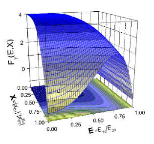
Figure 1: $F_{\gamma}(E,X)$ (as given by Eq. 18) spanning the full allowable range of the parameters $X$ and $E$ (defined in Eqs. 15 and 16). The function is optimized when simultaneously $E\rightarrow 0$ and $X\rightarrow 0$. As $X\rightarrow 1$ and $E\rightarrow 0$ or $E\rightarrow 1$ the function becomes negative, corresponding to a negative value of the second hyperpolarizability.

This result agrees with the quantum limit obtained from the traditional Orr and Ward SOS expression.KuzTHyper

Thus, we can conclude that when only three levels contribute to the nonlinear response, the dipole-free and the traditional SOS expressions for the second hyperpolarizability - when simplified using the sum rules - become the same, leading to the same quantum limits. We should point out that the quantum limits are obtained by assuming that the response is dominated by the contributions of three overlapping states, an ansatz that has been extensively verified numerically using Monte Carlo methodskuzkuz as well as potential energy optimization.zhoukuzwat There are no assumptions about the symmetry properties of the states. However, this does not imply that symmetry plays no role in he optimization of the second hyperpolarizability. The symmetry properties of the system will determine whether or not the optimal distribution of excited energies and transition dipole moments can be achieved. Mathematically, symmetries will impose further constraints on the parameters, which will make $\gamma$ smaller. We note that the quantum limit is negative for the centrosymmetric system, and is one-quarter of the positive limit that is obtained for an asymmetric molecule.

III.2 The particle in a box

In this section, we test the convergence of the expressions in the case of two exactly solvable quantum mechanical systems: the “particle in a box” and the “clipped harmonic oscillator”. For simplicity, we will first perform our calculations in the off-resonance regime.

The unperturbed states that we will use for our calculation of the second hyperpolarizability are the solutions of the one-dimensional time-independent Schrödinger equation:

$$-\frac{\hbar^{2}}{2m}\frac{\partial^{2}\Psi(x)}{\partial x^{2}}+V(x)\Psi(x)=E\Psi(x).$$ (20)

The potential that characterizes the particle in a box is zero inside the box of length $L$ and infinite, otherwise. The solutions are given by:

$$\Psi_{k}^{pb}=\sqrt{\frac{2}{L}}\sin\left(\frac{(k+1)\pi x}{L}\right),$$ (21)

with $k=0,1,2,3,\dots$ The corresponding energies are:

$$E_{k}=\frac{\hbar^{2}\pi^{2}}{2mL^{2}}(k+1)^{2},$$ (22)

where $m$ is the mass of the particle (in this case the electron mass). These solutions are substituted into the expressions for the diagonal component of the second hyperpolarizability (Eqs. 1 and 8) to study the convergence of both series as a function of number of excited levels included in the sum.

In the off-resonance regime, Eq. 1 becomes:

$$\gamma_{xxxx}=2e^{4}\left(2{\sum_{lmn}^{\infty}}^{\prime}\frac{x_{0l}\bar{x}_{lm}\bar{x}_{mn}x_{n0}}{E_{l0}E_{m0}E_{ng}}-{\sum_{mn}^{\infty}}^{\prime}x_{0m}^{2}x_{0n}^{2}\left\{\frac{1}{E_{m0}^{2}E_{n0}}+\frac{1}{E_{n0}^{2}E_{m0}}\right\}\right),$$ (23)

and Eq. 8 is given by:

$$\gamma_{xxxx} = 2e^{4}\left(2{\sum_{n}^{\infty}}^{\prime}{\sum_{m\neq n}^{\infty}}^{\prime}{\sum_{l\neq n}^{\infty}}^{\prime}\left\{\frac{(2E_{m0}-E_{n0})(2E_{l0}-E_{n0})}{E_{n0}^{5}}-\frac{(2E_{l0}-E_{n0})}{E_{m0}E_{n0}^{3}}\right\}x_{0m}x_{mn}x_{nl}x_{l0}\right.$$

$$+ 2{\sum_{n}^{\infty}}^{\prime}{\sum_{m\neq n}^{\infty}}^{\prime}{\sum_{l\neq m}^{\infty}}^{\prime}\left\{\frac{1}{E_{l0}E_{m0}E_{n0}}-\frac{(2E_{l0}-E_{n0})}{E_{m0}^{3}E_{n0}}\right\}x_{0l}x_{lm}x_{mn}x_{n0}$$

$$- \left.{\sum_{m}^{\infty}}^{\prime}{\sum_{n}^{\infty}}^{\prime}\left\{\frac{1}{E_{m0}^{2}E_{n0}}+\frac{1}{E_{n0}^{2}E_{m0}}\right\}x_{0m}^{2}x_{0n}^{2}\right).$$

The numerical evaluation of the diagonal component of the second hyperpolarizability as given by Eq. 23 or Eq. LABEL:eq:dipoleoff respectively, is performed by dividing every contribution in the sum by the quantum limit (Eq. 19). For the particle in a box, a general term in the sum can be rewritten as:

$$e^{4}\frac{x_{0l}x_{lm}x_{mn}x_{n0}}{E_{l0}E_{m0}E_{n0}}=\frac{3^{5}}{\pi^{4}}\gamma_{xxxx}^{\mbox{\tiny{off-max}}}\cdot\frac{g^{PB}_{0l}g^{PB}_{lm}g^{PB}_{mn}g^{PB}_{n0}}{f^{PB}_{l0}f^{PB}_{m0}f^{PB}_{n0}},$$ (25)

where we have used defined the following dimensionless functions:

$$g^{PB}_{mn} = \int_{0}^{\pi}\sin\left((m+1)y\right)\cdot y\cdot\sin\left((n+1)y\right)dy,$$ (26)

$$f^{PB}_{n0} = n(n+2).$$ (27)

The convergence of the two series in the off-resonance regime is shown in Fig. 2. When including the contribution of the first 10 states, the relative difference between traditional SOS expression for the second hyperpolarizability (Eq. 1) and the dipole-free expression (Eq. 8) is of the order of $5\times 10^{-4}$. With 50 states, the two expressions converge to the same value of:

$$\frac{\gamma^{\mbox{\tiny{off-PB}}}_{xxxx}}{\gamma^{\mbox{\tiny{off-max}}}_{xxxx}}=-0.08936.$$ (28)

Interestingly, the average value (also shown in Fig. 2) is more accurate when as few as three states are included in the sum. This is because, for the particular case of the particle in a box, if not enough states are included in the sums, the traditional SOS expression tends to underestimate while the dipole-free expressions tends to overestimate $\gamma$. In this case, with few excited states, using the average value yields a more reliable estimation of the second hyperpolarizability. This same result was found for the first hyperpolarizabilityKuzykNew and for studies used in modeling real molecules.champ

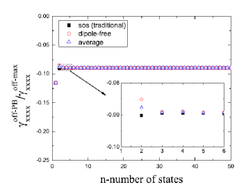
Figure 2: Convergence of the normalized SOS expressions as a function of the number of states in the sum for the particle in a box. Both the traditional SOS expression (Eq. 1) and the dipole-free expression (Eq. 8) converge quickly to the exact value given by Eq. 28. For completeness, we also plot the normalized average value of the two expressions, which converges more rapidly as a function of the number of states than the traditional and dipole-free expressions alone. The inset shows a mgnified view of the region indicated by the dash boxes.

III.3 The clipped harmonic oscillator

Another exactly solvable system is the clipped harmonic oscillator, whose potential energy function is given by:Ghatak

$$V(x)=\left\{\begin{array}[]{cc}\infty&\mbox{if $x<0$},\\ \frac{m\omega^{2}x^{2}}{2}&\mbox{if $x\geq 0$}\end{array}\right.$$ (29)

where $\omega$ has dimensions of frequency.

Introducing the dimensionless variable:

$$\xi=\sqrt{\frac{m\omega}{\hbar}}x,$$ (30)

the solutions are expressed as:

$$\Psi_{k}^{cho}=\left\{\begin{array}[]{cc}0&\mbox{if $\xi<0$},\\ (2^{2k}(2k+1)!)^{-1/2}\left(\frac{m\omega}{\pi\hbar}\right)^{1/4}\exp(-\xi^{2}/\omega)\,H_{2k+1}(\xi)&\mbox{if $\xi\geq 0$}\end{array}\right.$$ (31)

where $H_{k}(\xi)$ is the $k^{th}$ order Hermite Polynomial, and the energies are given by:

$$E_{k}=\hbar\omega\left(2k+\frac{3}{2}\right),$$ (32)

with $k=0,1,2,3,\dots$

For the clipped harmonic oscillator, a general term in the sum can be rewritten as:

$$e^{4}\frac{x_{0l}x_{lm}x_{mn}x_{n0}}{E_{l0}E_{m0}E_{n0}}=\frac{\gamma_{xxxx}^{\mbox{\tiny{off-CHO}}}}{\pi^{2}}\cdot\frac{g^{CHO}_{1(2l+1)}g^{CHO}_{(2l+1)(2m+1)}g^{CHO}_{(2m+1)(2n+1)}g^{CHO}_{(2n+1)1}}{l\cdot m\cdot n},$$ (33)

where we have defined the following dimensionless function:

$$g_{mn}^{CHO}=(2^{n-1}n!)^{-1/2}(2^{m-1}m!)^{-1/2}\int_{0}^{\infty}H_{n}(x)xH_{m}(x)dx.$$ (34)

The convergence of the two series in the off-resonance regime is shown in Fig. 3. In this case, it takes more terms to reach convergence than for the particle in a box. For 50 states, the relative difference between the traditional SOS expression (Eq. 1) and the dipole-free expression (Eq. 8) is of the order of $2\times 10^{-2}$. The traditional SOS expression converges faster to the final value:

$$\frac{\gamma^{\mbox{\tiny{off-CHO}}}_{xxxx}}{\gamma^{\mbox{\tiny{off-max}}}_{xxxx}}=-0.00842.$$ (35)

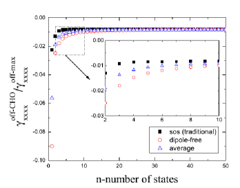
Figure 3: Convergence of the normalized SOS expressions as a function of the number of states in the sum for the clipped harmonic oscillator. Both the traditional SOS expression (Eq. 1) and the dipole-free expression (Eq. 8) converge slowly to the exact value given by Eq. 35. For completeness, we also plot the normalized average value of the two expressions. The inset shows a magnified view of the region indicated by the dash boxes.

III.4 Dispersion studies using 6 excited levels

In this section, we investigate the convergence of the dispersion of the two forms of the second hyperpolarizability. In particular, we will treat two separate cases: two photon absorption (TPA) - which is related to the imaginary part of $\gamma$ and used in a broad range of applications such as photodynamic cancer therapies and 3D photolithography,CancerMaterials ; Cancer ; PKawata ; PCumpston and the optical Kerr effect(OKE) - which is related to the real part of $\gamma$ and widely used in characterizing materials with potential applications in all-optical switching.Oke ; gates ; shutters We begin by evaluating Eqs. 3 and 4 and including only the first 6 excited states.

To get the typical qualitative behavior of real large chromophores, we choose $E_{10}=1eV$. All the linewidths are given by $\Gamma_{n}=0.1eV$ which is also typical for organic chromophores. We normalize the second hyperpolarizability by dividing by the off-resonance limit for $E_{10}=1eV$.

Fig. 4 shows the dispersion predicted by the traditional sum-over-states expression and the dipole-free expression for the imaginary part of the second hyperpolarizability as s function of the incident photon energy. Note that $Im[\gamma]$ is related to the two photon absorption cross-section. The agreement between the two expressions is excellent everywhere with the exception of the third resonance (see inset in Fig. 4), where the two differ by less than 20%.

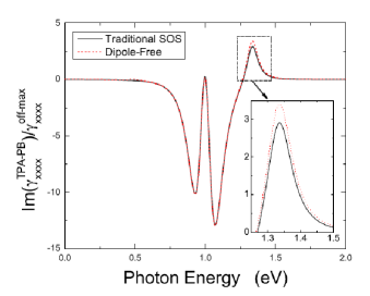
Figure 4: The normalized imaginary part of the two photon absorption second hyperpolarizability as a function of the incident photon energy for a 7-level model for the particle in a box using the traditional sum-over-states and the dipole-free expressions. The inset shows a magnified view of the region indicated by the dashed box. $E_{10}=1eV$.

Next we compare the two expressions for the real part of the second hyperpolarizability - which is related to the optical Kerr effect - as a function of the fundamental photon energy for the particle in a box . The results are plotted in Fig. 5. In this case, for 6 excited states, the two expressions differ by as much as a factor of 2 in some regions (see insets). Although the qualitative behavior is the same, this type of discrepancy should be considered when experimental data is analyzed using a limited number of terms in the sum-over-states expressions.

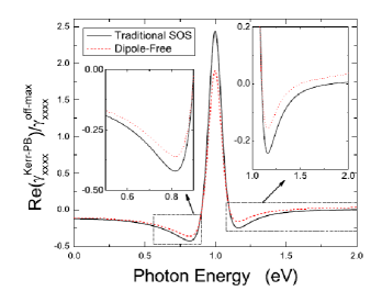
Figure 5: The normalized real part of the Kerr effect second hyperpolarizability as a function of the incident photon energy for a 7-level model for the particle in a box using the traditional sum over states and the dipole-free expressions. The insets show a magnified view of the region indicated by the dashed boxes. $E_{10}=1eV$.

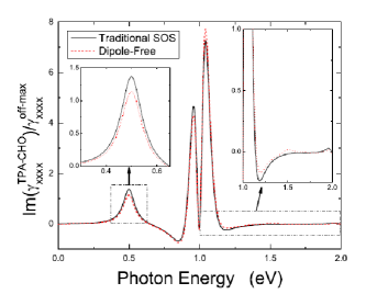
Figure 6: The normalized imaginary part of the two photon absorption second hyperpolarizability as a function of the incident photon energy for a 7-level model for the clipped harmonic oscillator using the traditional sum-over-states and the dipole-free expressions. The inset shows a magnified view of the region indicated by the dashed boxes. $E_{10}=1eV$.

Next we consider the dispersion predicted by the traditional sum-over-states expression and the dipole-free expression for the imaginary part of the two photon absorption second hyperpolarizability as a function of the fundamental photon energy for the clipped harmonic oscillator. The results are plotted in Fig. 6. The agreement between the two expressions is good, differing only near the resonances. Finally, Fig. 7 shows the dispersion predicted by the two expressions for the Kerr effect second hyperpolarizability as a function of the fundamental photon energy for the clipped harmonic oscillator. For 6 excited states, the two expressions differ substantially only in the vicinity of a resonance (see insets).

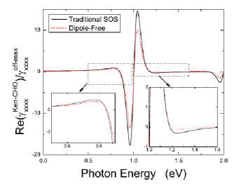
Figure 7: The normalized real part of the Kerr effect second hyperpolarizability as a function of the incident photon energy for a 7-level model for the clipped harmonic oscillator using the traditional sum-over-states and the dipole-free expressions. The insets show a magnified view of the region indicated by the dashed boxes. $E_{10}=1eV$.

IV Convergence of the dipole-free expression

In this section we will study the convergence of the dipole-free series expression (Eq. 8) as a function of the number of excited states included in the sum. The convergence is studied as a function of photon energy for two photon absorption and the Kerr effect, using the particle in a box and the clipped harmonic oscillator as model quantum systems. Again, in order to get the typical qualitative behavior of large real chromophores, we choose $E_{10}=1eV$, and all the linewidths are given by $\Gamma_{n}=0.1eV$ which is also typical for organic chromophores. Also, we normalize the second hyperpolarizability by dividing by the off-resonance limit for $E_{10}=1eV$.

In all the cases it is found that after including about 15 excited states in the sum the expression converges even in the vicinity of a resonance. In order to get a better understanding of the convergence behavior of the expressions we will use the particle in a box model as a test for convergence, once we take into account symmetry considerations.

For clarity, we will look again to the expression for the second hyperpolarizability that separates explicitly dipolar terms from dipole-free terms:

$$e^{4}{\sum_{n}^{\infty}}^{\prime}\left({\sum_{m}^{\infty}}^{\prime}\left({\sum_{l}^{\infty}}^{\prime}\frac{x_{0l}\bar{x}_{lm}\bar{x}_{mn}x_{n0}}{D_{lmn}^{-1}}\right)\right) =$$

$$e^{4}{\sum_{n}^{\infty}}^{\prime}\frac{(\Delta x_{n0}x_{0n})^{2}}{D^{-1}_{nnn}}+e^{4}{\sum_{n}^{\infty}}^{\prime}{\sum_{m\neq n}^{\infty}}^{\prime}\frac{\Delta x_{m0}x_{0m}x_{mn}x_{n0}}{D_{mmn}^{-1}} + e^{4}{\sum_{n}^{\infty}}^{\prime}{\sum_{l\neq n}^{\infty}}^{\prime}\frac{\Delta x_{n0}x_{0l}x_{ln}x_{n0}}{D_{lnn}^{-1}}$$

$$+e^{4}{\sum_{n}^{\infty}}^{\prime}{\sum_{m\neq n}^{\infty}}^{\prime}{\sum_{l\neq m}^{\infty}}^{\prime}\frac{x_{0l}x_{lm}x_{mn}x_{n0}}{D_{lmn}^{-1}} - e^{4}{\sum_{mn}^{\infty}}^{\prime}\frac{x_{0m}x_{m0}x_{0n}x_{n0}}{D^{-1}_{mn}}.$$ (36)

For a system whose symmetry demands that all dipole moments vanish, i.e. $\Delta x_{m0}=0$ for $m=1,2,3,\cdots$, such as the the centrosymmetric system of a particle in a box or molecules with octupolar symmetry (i.e. no dipole moment but non-centrosymmetric), the first three terms must each vanish. Numerically, when we use the dipole-free expression to model such systems that are centrosymmetric, which demands that all dipole moments vanish, the contributions from the first three terms are precisely zero only when an infinite number of terms are included in the sum.

It is useful to consider how many states are needed in order for each of these dipolar terms, written in our new non-dipolar form, to vanish. We define the partial sums $S_{1}$, $S_{2}$ and $S_{3}$ and $S_{4}$ as:

$$S_{1} = e^{4}{\sum_{n}^{\infty}}^{\prime}\frac{(\Delta x_{n0}x_{0n})^{2}}{D^{-1}_{nnn}}=e^{4}{\sum_{n}^{\infty}}^{\prime}{\sum_{m\neq n}^{\infty}}^{\prime}{\sum_{l\neq n}^{\infty}}^{\prime}\frac{(2E_{m0}-E_{n0})(2E_{l0}-E_{n0})}{E_{n0}^{2}}\cdot\frac{x_{0m}x_{mn}x_{nl}x_{l0}}{D_{nnn}^{-1}},$$ (37)

$$S_{2} = e^{4}{\sum_{n}^{\infty}}^{\prime}{\sum_{m\neq n}^{\infty}}^{\prime}\frac{\Delta x_{m0}x_{0m}x_{mn}x_{n0}}{D_{mmn}^{-1}}=-e^{4}{\sum_{n}^{\infty}}^{\prime}{\sum_{m\neq n}^{\infty}}^{\prime}{\sum_{l\neq m}^{\infty}}^{\prime}\frac{(2E_{l0}-E_{m0})}{E_{m0}}\cdot\frac{x_{0l}x_{lm}x_{mn}x_{n0}}{D_{mmn}^{-1}},$$ (38)

$$S_{3} = e^{4}{\sum_{n}^{\infty}}^{\prime}{\sum_{l\neq n}^{\infty}}^{\prime}\frac{\Delta x_{n0}x_{0l}x_{ln}x_{n0}}{D_{lnn}^{-1}}=-e^{4}{\sum_{n}^{\infty}}^{\prime}{\sum_{l\neq n}^{\infty}}^{\prime}{\sum_{m\neq n}^{\infty}}^{\prime}\frac{(2E_{m0}-E_{n0})}{E_{n0}}\cdot\frac{x_{0l}x_{ln}x_{nm}x_{m0}}{D_{lnn}^{-1}},$$ (39)

$$S_{4} = e^{4}{\sum_{n}^{\infty}}^{\prime}{\sum_{m\neq n}^{\infty}}^{\prime}{\sum_{l\neq m}^{\infty}}^{\prime}\frac{x_{0l}x_{lm}x_{mn}x_{n0}}{D_{lmn}^{-1}}-e^{4}{\sum_{mn}^{\infty}}^{\prime}\frac{x_{0m}x_{m0}x_{0n}x_{n0}}{D^{-1}_{mn}}.$$ (40)

Clearly,  for systems where there is no change in the dipole moment between the ground and excited states, the dipole-free expression will converge when simultaneously: $S_{1}\rightarrow 0$, $S_{2}\rightarrow 0$ and $S_{3}\rightarrow 0$ and $S_{4}\rightarrow\gamma_{xxxx}(-\omega_{\sigma};\omega_{1},\omega_{2},\omega_{3})$. We will test these conditions numerically using the particle in a box as a model of a centrosymmetric potential with no dipole moment.

First we consider two photon absorption and study the convergence of $S_{1}$ (Eq. 37), $S_{2}$ (Eq. 38), $S_{3}$ (Eq. 39) and $S_{4}$ (Eq. 40) as a function of the number of excited states for a range of different photon energies. The results are shown in Fig. 8. Clearly, for all cases, few excited states (from 2 to 5) are needed to get good convergence when away from resonance. While $S_{1}$ also converges in the resonant regime after 10 excited states are included more excited states (up to 20) are required for convergence of $S_{2}$ and $S_{3}$ near resonance (see insets). Finally we look at the convergence of $S_{4}$ (Eq. 40), which as we have seen, converges to the exact value of the second hyperpolarizability for systems with no permanent dipole moment, such as the particle in a box. Surprisingly, this expression is shown to converge rapidly as a function of number of excited states included in the sum, even on resonance. In fact, it is clear from the plot that only 2 excited levels might suffice to study the qualitative behavior of the second hyperpolarizability even close to the resonances.

Figure 8: The normalized imaginary part of the partial sums $S_{1}$ (top-left), $S_{2}$ (top-right), $S_{3}$ (bottom-left) and $S_{4}$ (bottom-right) for two photon absorption as a function of the incident photon energy. The number of states included in the sum is shown in the figure legends. The particle in a box is used as a model centrosymmetric system with vanishing dipole moments, and therefore as the sums converge we must have $S_{1}\rightarrow 0$, $S_{2}\rightarrow 0$, $S_{3}\rightarrow 0$ and $Im(S_{4})=Im(\gamma_{xxxx}^{\mbox{\tiny{TPA-PB}}})$. The insets show a magnified view of the regions indicated by the dashed boxes.

Similarly, we next consider the Kerr effect and study the convergence of $S_{1}$ (Eq. 37), $S_{2}$ (Eq. 38) and $S_{3}$ (Eq. 39) and $S_{4}$ (Eq. 40) as a function of the number of excited states for a range of different photon energies. The results are shown in Fig. 9. Again, few excited levels are needed for convergence away from resonance, although more excited states (up to 20) are required for convergence near resonance. As in the case of the two photon absorption second hyperpolarizability, $S_{4}$ (Eq. 40), which is the only terms that contributes to the second hyperpolarizability for the centrosymmetric potential given by the particle in a box is shown to converge rapidly as a function of number of excited states included in the sum, even in the resonant regime.

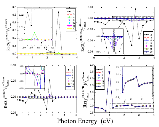
Figure 9: The normalized real part of the partial sums $S_{1}$ (top-left), $S_{2}$ (top-right), $S_{3}$ (bottom-left) and $S_{4}$ (bottom-right) for the Kerr effect second hyperpolarizability as a function of the incident photon energy. The number of states included in the sum is shown in the figure legends. The particle in a box is used as a model centrosymmetric system with vanishing dipole moments, and therefore as the sums converge we must have $S_{1}\rightarrow 0$, $S_{2}\rightarrow 0$, $S_{3}\rightarrow 0$ and $Re(S_{4})=Re(\gamma_{xxxx}^{\mbox{\tiny{KERR-PB}}})$. The insets show a magnified view of the region indicated by the dashed boxes.

For completeness, we also study the convergence of the expressions for the two photon absorption process and the Kerr effect using the clipped harmonic oscillator as a quantum model. As shown by the results in Fig. 10 the expressions do not converge as rapidly as did the particle in a box; but when 15 excited states are included in the sum, the spectral features do not change quantitatively.

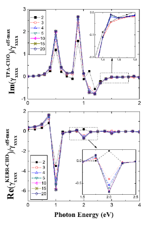
Figure 10: The normalized imaginary part of the two photon absorption second hyperpolarizability (top) and the normalized real part of the Kerr effect second hyperpolarizability(bottom) as a function of the incident photon energy. The number of states included in the sum is shown in the figure captions. The clipped harmonic oscillator is used as a model, with $E_{10}=1eV$. The insets show a magnified view of the regions indicated by the dashed boxes.

All of our results show that the dipole-free expression converges even in the resonant regime when enough excited states (up to 20) are included in the expression. We have also shown that for systems with no dipole moments (such as octupolar molecules or the particle in a box) the dipole-free expression for the second hyperpolarizability collapses to Eq. 40 (which we will call the reduced dipole-free expression), since all the other terms vanish. In this case, the reduced dipole-free expression converges when only a few excited states are included in the sum.

V Conclusions

We have developed an expression that eliminates the explicit dependence on dipolar terms but is physically equivalent to the traditional SOS expression for the second hyperpolarizability. The equivalence between the dipole-free and the traditional SOS expressions is demonstrated by calculating the quantum limits and studying the convergence of the series with the exact wavefunctions of two quantum systems: the particle in a box and the clipped harmonic oscillator. In both cases, when a large number of states is included, the two expressions are identical. However, the average of the two expressions converges faster than the individual expressions.

Since the average between the two expressions appears to be a better approximation to molecular dispersion, the average may make it possible to use limited-state models when interpreting experimental dispersion data. Since accurate measurements of transition moments between excited states are difficult and tedious, the averaged second hyperpolarizability can be a useful tool for modeling the second hyperpolarizability when only limited information is available about the excited states of a particular system.

To test the convergence between the two expressions, we have evaluated them in the resonant regime in two model systems: the particle in a box - which is a symmetric potential with no change in dipole moment; and the clipped harmonic oscillator - an asymmetric potential. This allows us to determine the role of symmetry. In both cases, we study the dispersion of the second hyperpolarizability near resonance, where - based on the different energy denominators - one would expect the differences between the two expressions to be the least consistent. The reduced dipole-free expression has been introduced for systems with no dipole moment. Such an expression might be most appropriate when experimental results are interpreted since it requires the minimum number of molecular parameters.

In conclusion, the dipole-free expression is an alternative to the traditional SOS expression that increases the theoretical pallet available to quantum chemists. It is more direct in certain theoretical problems such as its application to the derivation of a more-rigorous calculation of the fundamental limits of the third-order susceptibility. It provides a tool to assess the convergence of truncated SOS calculations, can be used to determine the accuracy of molecular-orbital calculations of nonlinear susceptibilities, and can be used to refine limited-state models to interpret experimental results. And, it may be more naturally applicable to the analysis of specific systems such as octupolar structures.ZyssJCP ; ZyssCR ; VerbiestJACS ; VerbiestOL ; Bidault ; Ledoux-Rak ; Ratera ; LeBozec ; Zyss1993

Acknowledgements: JPM acknowledges the Fund for Scientific Research Flanders (FWO) and the support from the Division of Molecular and Nanomaterials at the Department of Chemistry in KULeuven. MGK thanks the National Science Foundation (ECS-0354736) and Wright Paterson Air Force Base for generously supporting this work.

References

• (1) R. W. Boyd, “Nonlinear Optics”, Academic Press (2002).
• (2) B. J. Orr and J. F. Ward, Molecular Physics, 20, 513-526 (1971).
• (3) “Characterization Techniques and Tabulations for Organic Nonlinear Optical Materials”, M. G. Kuzyk & C. W. Dirk, Editors. New York : Marcel Dekker (1998).
• (4) J. L. Oudar and D. S. Chemla, J. Chem. Phys. 66, 2664-2668 (1977).
• (5) C. W. Dirk, L. T. Cheng, and M. G. Kuzyk, Int. J. Quant. Chem. 43, 27 (1992).
• (6) M. Nakano and K. Yamaguchi, Chem. Phys. Lett. 206, 285 (1993).
• (7) F. Meyers, S. R. Marder, B. M. Pierce and J. L. Brédas, Chem. Phys. Lett. 228 172 (1994).
• (8) J. Pérez-Moreno and M. G. Kuzyk, J. Chem. Phys. 123, 194101 (2005).
• (9) M. G. Kuzyk, Phys. Rev. A 72, 053819 (2005).
• (10) M. G. Kuzyk, J. Chem. Phys. 125, 154108 (2006).
• (11) B. Champagne and B. Kirtman, J. Chem. Phys. 125, 024101 (2006).
• (12) M. G. Kuzyk, Opt. Lett. 25, 1183-1185 (2000).
• (13) B. Champagne and B. Kirtman, Phys. Rev. Lett. 95, 109401 (2005).
• (14) M. G. Kuzyk, Phys. Rev. Lett. 95, 109402 (2005).
• (15) M. G. Kuzyk, Phys. Rev. Lett. 85, 1218 (2000).
• (16) M. G. Kuzyk, Phys. Rev. Lett. 90, 039902 (2003).
• (17) M. G. Kuzyk, J. Chem. Phys. 119, 8327 (2003).
• (18) M. G. Kuzyk, Phys. Rev. Lett. 95, 109402 (2005).
• (19) K. Tripathi, P. Moreno, M. G. Kuzyk, B. J. Coe, K. Clays, and A. M. Kelley, J. Chem. Phys. 121, 7932 (2004).
• (20) Mark C. Kuzyk and Mark G. kuzyk, J. Opt. Soc. Am B, in press.
• (21) Juefei Zhou, Urszula B. Szafruga, David S. Watkins, and Mark G. Kuzyk, Phys. Rev. A 76, 053831 (2007).
• (22) “Quantum Mechanics: Theory and Applications”, A. K. Ghatak and S. Lokanathan, pp. 190-196. Springer (2004).
• (23) A. Karotki, M. Drobizhev, Y. Dzenis, P. N. Taylor, H. L. Anderson, and A. Rebane, Phys. Chem. Phys. 6, 7 (2004).
• (24) I. Roy, O. T. Y., H. E. Pudavar, E. J. Bergey, A. R. Oseroff, J. Morgan, T. J. Dougherty, and P. N. Prasad, J. Am. Chem. Soc. 125, 7860 (2003).
• (25) S. Kawata, H. -B. Sun, T. Tanaka, and K. Takada, Nature 412, 697 (2001).
• (26) B. H. Cumpston, S. P. Ananthavel, S. Barlow, D. L. Dyer, J. E. Ehrlich, L. L Erskine, A. A. Heikal, S. M. Kuebler, I. -Y. S. Lee, D. McCord-Maughon, et al., Nature 398, 51 (1999).
• (27) G. Mayer and F. C. Gires, C. R. Acad. Sc. Paris, 258, 2039 (1964).
• (28) M. A. Duguay and J. W. Hanse, Appl. Phys. Lett., 15, 192 (1969).
• (29) H. J. Coles and B. R. Jennings, Phil. Mag., 32, 105 (1975).
• (30) J. Zyss, J. Chem. Phys. 98, 6583 (1993).
• (31) J. Zyss and I. Ledoux, Chem. Rev. 94, 77 (1994).
• (32) T. Verbiest, K. Clays, C. Samyn, J. Wolff, D. Reinhoudt and A. Persoons, J. Am. Chem. Soc. 116, 9320 (1994).
• (33) T. Verbiest, K. Clays, A. Persoons, F. Meyers and J. -L. Brédas, Opt. Lett. 18, 525 (1993).
• (34) S. Bidault, S. Brasselet, J. Zyss et al., J. Chem. Phys. 126, 34312 (2007).
• (35) I. Ledoux-Rak, J. Zyss, T. Le Bouder et al., Journal of Luminescence 111, 307 (2005)
• (36) I. Ratera, S. Marcen, S. Montant et al., Chem. Phys. Lett. 363 245 (2002).
• (37) H. Le Bozec, T. Le Bouder, O. Maury et al., Adv. Mat. 13 1677 (2001).
• (38) J. Zyss, J. Chem. Phys. 98, 6583 (1993).