Effects of the triaxial deformation and pairing correlation on the proton emitter ¹⁴⁵Tm

Abstract

The ground-state properties of the recent reported proton emitter ¹⁴⁵Tm have been studied within the axially or triaxially deformed relativistic mean field (RMF) approaches, in which the pairing correlation is taken into account by the BCS-method with a constant pairing gap. It is found that triaxiality and pairing correlations play important roles in reproducing the experimental one proton separation energy. The single-particle level, the proton emission orbit, the deformation parameters $\beta=0.22$ and $\gamma=28.98^{\circ}$ and the corresponding spectroscopic factor for ¹⁴⁵Tm in the triaxial RMF calculation are given as well.

I Introduction

Proton-rich nuclei display many interesting structural properties which are important both for nuclear physics and astrophysics. These nuclei are characterized by exotic decay modes, such as the direct emission of charged particles from the ground state, and $\beta$-decays with large Q-values. The decay via direct proton emission provides a unique insight into the structure of nuclei beyond the drip line limit. The evolution of the single-particle structure, nuclear shapes and masses can be deduced from measured properties of proton emission Woods97 .

Proton emission in both spherical and deformed systems has been studied extensively in the past decades Delion06 . For the spherical proton emitter, a simple WKB estimation of the transmission through the Coulomb and centrifugal barriers could give the correct order of magnitude of the decay rates and the angular momentum of the decaying state  Feix83 ; Iriondo86 ; Davids97 ; Aberg97 . Most of the proton emitters in the rare earth region, which are predicted to have large static quadrupole deformations Moeller95 are analyzed by a particle-coupled core model with the unbound proton interacting with an axially symmetric deformed core Kadmensky96 ; Ferreira97 ; Davids98 ; Maglione98 ; Maglione99 ; Sonzogni99 ; Rykaczewski99 ; Barmore00 ; Esbensen00 ; Seweryniak01 . Such an analysis over the past several years turned out to be a good description of the ground-state properties of axially deformed rare-earth proton emitters.

Recently, the proton emission from triaxial nuclei has drawn lots of attention Kruppa04 ; Davids04 ; Delion04 ; Arumugam07 ; Seweryniak07 . Specific combinations of single-particle orbitals near the Fermi surface can lead to a propensity toward triaxial shapes as illustrated by recent calculations of the additional binding energy due to non-axial degrees of freedom Moeller06 , which revealed several ”islands” of triaxiality throughout the nuclear chart. In Ref. Davids04 , the static triaxial deformation was introduced in the adiabatic coupled channels method in order to investigate proton emission from ¹⁴¹Ho($7/2^{-}$). The total decay rate and the 2+ branching ratio, however, were found to be good agreement with experimental data only for the triaxial angle $\gamma<5^{\circ}$. The importance of triaxial deformation in proton emitters ¹⁶¹Re and ¹⁸⁵Bi was pointed out in Ref. Delion04 , where the decay widths were found to be very sensitive to the $\gamma$ deformation. However, the sensitivity of decay widths in ¹⁶¹Re and ¹⁸⁵Bi on the triaxial deformation was questioned in a recent paper reporting a non-adiabatic quasipartilce calculation Arumugam07 . Instead, the pairing effect was found to have a more significant influence. In Ref. Seweryniak07 , the quasiparticle-coupled core model has been used to address the important role of the gamma degree of freedom in the prediction of the proton decay rate and the spectrum of excited states in the proton emitter ¹⁴⁵Tm.

It should be pointed out that the nuclear potentials in the (quasi)particle-coupled core model are tuned to fit the measured energy of the decaying state Esbensen00 . In particular, it cannot provide any information about the microscopic structure properties of proton emitters.

Approaches based on concepts of non-renormalizable effective relativistic field theories and density functional theory provide a very reliable theoretical framework for studies of nuclear structure phenomena at and far from the valley of $\beta$-stability. In particular, the relativistic mean field (RMF) theory, which can take into account the spin-orbit coupling naturally, has been successfully applied in analysis of nuclear structure over the whole periodic table, from light to superheavy nuclei with a few universal parameters Serot86 ; Reinhard89 ; Ring96 ; Vretenar05 ; Meng06 . The application of RMF theory with the restriction of axial symmetry to study the properties of proton emitter has already been done Vretenar99 ; Lalazissis99 ; Geng04 . In general, the predicted location of the proton drip line, the ground-state quadrupole deformations, one proton separation energies at and beyond the drip line, the deformed single-particle orbit occupied by the odd valence proton, and the corresponding spectroscopic factor are in good agreement with the experimental data. However, the influence of triaxiality on proton emitters has not been investigated in the microscopic self-consistent RMF approach. Here in this paper, the influences of $\gamma$ deformation degree of freedom and pairing correlations on proton emitters ¹⁴⁵Tm will be studied within the triaxial deformed RMF approach.

The paper is arranged as follows. In Sec. II, a brief introduction of the RMF approach will be given. Both axial and triaxial calculations with pairing correlation are carried out to investigate the properties of proton emitter ¹⁴⁵Tm in Sec. III, including total energy, quadrupole deformations, one-proton separation energy, the potential of the valence proton, and the corresponding spectroscopic factor. Finally, our conclusions and summary are given in Sec. IV.

II The relativistic mean field theory

The starting point of the RMF theory with meson-exchange providing nucleon-nucleon interaction is the standard effective Lagrangian density constructed with the degrees of freedom associated with the nucleon field ($\psi$), two isoscalar meson fields  ($\sigma$ and $\omega_{\mu}$), the isovector meson field ($\vec{\rho}_{\mu}$) and the photon field ($A_{\mu}$),

$$\begin{split}{\cal L}=~{}&\bar{\psi}\left[i\gamma^{\mu}\partial_{\mu}-m-g_{\sigma}\sigma-g_{\omega}\gamma^{\mu}\omega_{\mu}-g_{\rho}\gamma^{\mu}\vec{\tau}\cdot\vec{\rho}_{\mu}-\frac{1}{2}e(1-\tau_{3})\gamma^{\mu}A_{\mu}\right]\psi\\ &+\frac{1}{2}\partial^{\mu}\sigma\partial_{\mu}\sigma-U_{\sigma}(\sigma)-\frac{1}{4}\Omega^{\mu\nu}\Omega_{\mu\nu}+U_{\omega}(\omega_{\mu})-\frac{1}{4}\vec{R}^{\mu\nu}\cdot\vec{R}_{\mu\nu}+U_{\rho}(\vec{\rho}_{\mu})\\ &-\frac{1}{4}F^{\mu\nu}F_{\mu\nu},\end{split}$$ (1)

where $m$ and $m_{i}(g_{i})$ ($i=\sigma,\omega_{\mu},\vec{\rho}_{\mu}$) are the masses (coupling constants) of the nucleon and the mesons respectively and

$$\Omega^{\mu\nu} = \partial^{\mu}\omega^{\nu}-\partial^{\nu}\omega^{\mu},$$ (2a)

$$\vec{R}^{\mu\nu} = \partial^{\mu}\vec{\rho}^{\nu}-\partial^{\nu}\vec{\rho}^{\mu},$$ (2b)

$$F^{\mu\nu} = \partial^{\mu}A^{\nu}-\partial^{\nu}A^{\mu}$$ (2c)

are the field tensors of the vector mesons and the electromagnetic field. Here in this paper, we adopt the arrows to indicate vectors in isospin space and bold types for the space vectors. Greek indices $\mu$ and $\nu$ run over 0, 1, 2, 3, while Roman indices $i$, $j$, etc. denote the spatial components.

The nonlinear self-coupling terms $U_{\sigma}(\sigma)$, $U_{\omega}(\omega_{\mu})$, and $U_{\rho}(\vec{\rho}_{\mu})$ for the $\sigma$-meson, $\omega$-meson, and $\rho$-meson in the Lagrangian density (1) respectively have the following forms:

$$U_{\sigma}(\sigma) = \frac{1}{2}m_{\sigma}^{2}\sigma^{2}+\frac{1}{3}g_{2}\sigma^{3}+\frac{1}{4}g_{3}\sigma^{4},$$ (3a)

$$U_{\omega}(\omega_{\mu}) = \frac{1}{2}m_{\omega}^{2}\omega^{\mu}\omega_{\mu}+\frac{1}{4}c_{3}\left(\omega^{\mu}\omega_{\mu}\right)^{2},$$ (3b)

$$U_{\rho}(\vec{\rho}_{\mu}) = \frac{1}{2}m_{\rho}^{2}\vec{\rho}~{}^{\mu}\cdot\vec{\rho}_{\mu}.$$ (3c)

In the mean-field approximation, the correspondent energy functional is obtained as

$$\begin{split}E_{\text{RMF}}[\rho,\phi_{m}]=&\int d^{3}x{\rm Tr}\left[\beta\left({\mbox{\boldmath${\rm\gamma}$}}\cdot{\mbox{\boldmath${\rm p}$}}+m+g_{\sigma}\sigma+g_{\omega}\gamma_{\mu}\omega^{\mu}+g_{\rho}\gamma^{\mu}\vec{\tau}\cdot\vec{\rho}_{\mu}+\frac{1}{2}e(1-\tau_{3})\gamma^{\mu}A_{\mu}\right)\rho\right]\\ &+\int d^{3}x\left\{\frac{1}{2}\partial^{0}\sigma\partial_{0}\sigma-\frac{1}{2}\partial^{i}\sigma\partial_{i}\sigma+U_{\sigma}(\sigma)-\frac{1}{4}\Omega^{0\mu}\Omega_{0\mu}+\frac{1}{4}\Omega^{i\mu}\Omega_{i\mu}-U_{\omega}(\omega_{\mu})\right.\\ &~{}~{}~{}~{}~{}~{}~{}~{}~{}~{}~{}~{}~{}~{}\left.-\frac{1}{4}\vec{R}^{0\mu}\cdot\vec{R}_{0\mu}+\frac{1}{4}\vec{R}^{i\mu}\cdot\vec{R}_{i\mu}-U_{\rho}(\vec{\rho}_{\mu})-\frac{1}{4}F^{0\mu}F_{0\mu}+\frac{1}{4}F^{i\mu}F_{i\mu}\right\},\end{split}$$ (4)

where $\phi_{m}$ denotes $\{\sigma,\omega_{\mu},\vec{\rho}_{\mu},A_{\mu}\}$ respectively.

The equations of motion for the nucleon and the mesons can be obtained by requiring that the energy functional (4) be stationary with respect to the variations of $\rho$ and $\phi_{m}$,

$$\delta\left\{E_{\text{RMF}}[\rho,\phi_{m}]-{\rm Tr}(\epsilon\rho)\right\}=0,$$ (5)

where $\epsilon$ is a diagonal matrix, whose diagonal elements are the single particle energies. Using the variation $\delta\rho$ with respect to $\psi_{k}$, the stationary condition (5) leads to the Dirac equation,

$$[\mbox{\boldmath$\alpha$}\cdot{\mathbf{p}}+\beta(m+S+\gamma^{\mu}V_{\mu})]\psi_{k}=\epsilon_{k}\psi_{k}$$ (6)

for the nucleon. The scalar potential $S$ and vector potential $V_{\mu}$ in Eq. (6) are respectively,

$$S = g_{\sigma}\sigma,$$ (7a)

$$V_{\mu} = g_{\omega}\omega_{\mu}+g_{\rho}\vec{\tau}\cdot\vec{\rho}_{\mu}+\frac{1}{2}e(1-\tau_{3})A_{\mu}.$$ (7b)

The Klein-Gordon equations for the mesons and the photon are given by,

$$\partial_{\mu}\partial^{\mu}\phi_{m}+U^{\prime}(\phi_{m})=\pm S_{\phi_{m}},$$ (8)

where the $(+)$ sign is for vector fields and the $(-)$ sign for the scalar field. The source terms $S_{\phi_{m}}$ in Eq.(8) are sums of bilinear products of Dirac spinors

$$S_{\phi_{m}}=\left\{\begin{array}[]{ll}\sum\limits_{k>0}v^{2}_{k}\overline{\psi}_{k}\psi_{k},&\phi_{m}=\sigma\\ \sum\limits_{k>0}v^{2}_{k}\overline{\psi}_{k}\gamma_{\mu}\psi_{k},&\phi_{m}=\omega_{\mu}\\ \sum\limits_{k>0}v^{2}_{k}\overline{\psi}_{k}\gamma_{\mu}\vec{\tau}\psi_{k},&\phi_{m}=\vec{\rho}_{\mu}\\ \sum\limits_{k>0}v^{2}_{k}\overline{\psi}_{k}\gamma_{\mu}\frac{1-\tau_{3}}{2}\psi_{k},&\phi_{m}=A_{\mu}\end{array}\right.$$ (13)

where the sums run over only the positive-energy states ($k>0$) (i.e., no sea approximation) and the occupation probability of the single-particle energy level $k$, i.e., $v^{2}_{k}$, is evaluated within the BCS method. It is sufficient for proton-rich nuclei because of the attenuating effect of the Coulomb barrier on the spatial extent of the proton wave function, which limits the formation of proton halo.

III Results and discussion

The static Dirac equation (6) for the nucleon and Klein-Gordon equation (8) for the meson fields are solved by expansion on the cylindric (axially deformed RMF) or three-dimensional Cartesian (triaxially deformed RMF) harmonic oscillator basis with major shell numbers as $n_{\rm f}$ and $n_{\rm b}$ for the nucleons and mesons respectively. The equation of motion for the photon field is solved using the standard Green’s function method because of its long range. The parameter set PK1 Long04 is used throughout the calculation and the center-of-mass (c.m.) correction is taken into account by

$$E^{\rm mic}_{\rm cm}=\frac{1}{2mA}\langle\hat{\mathbf{P}}^{2}_{\rm cm}\rangle,$$ (14)

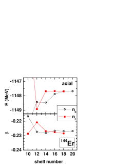
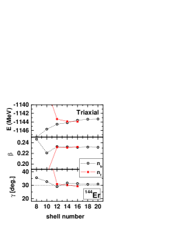
Figure 1: (Color online) The total energy, deformation parameters $\beta$ and $\gamma$ calculated in axially (left panel) and triaxially (right panel) deformed RMF with PK1 for ¹⁴⁴Er as functions of the number of expanded oscillator shells for the meson field $n_{\rm b}$ and the nucleon field $n_{\rm f}$.

where ${\mathbf{P}}_{\rm c.m.}$ is the total momentum of a nucleus with $A$ nucleons. In order to check the convergence of the results with the number of expanded oscillator shells for nucleons $n_{\rm f}$ and for mesons $n_{\rm b}$, the total energy, quadrupole deformation $\beta$ and $\gamma$ of ¹⁴⁴Er as functions of shell numbers are calculated with axially (left panel) and triaxially (right panel) deformed RMF approaches as shown in Fig. 1. It indicates that as long as $n_{\rm f}\geq 14,n_{\rm b}\geq 18$, the binding energies and the deformations are independent of the expanded shell numbers. Therefore in the following, $n_{\rm f}=14$ and $n_{\rm b}=20$ will be adopted. More details about the axially and triaxially deformed RMF approaches can be found in Ref. Gambhir90 and Refs. Hirata96 ; Yao06 respectively.

In order to get the pairing gaps for ¹⁴⁴Er and ¹⁴⁵Tm, we fit odd-even mass differences of around 120 nuclides Audi03 in the very proton-rich side ranging from La to Re by the four-point difference formula. The neutron and proton pairing gaps obtained are, $\Delta^{\rm est.}_{n}=13.7/\sqrt{A}$ and $\Delta^{\rm est.}_{p}=15.9/\sqrt{A}$ respectively, and the corresponding rms deviation with respect to experimentally known values are 0.17 and 0.16 MeV. Considering the blocking effect of odd valence proton, the proton pairing gap for ¹⁴⁵Tm is reduced by a factor $f$, ranging from zero to one in the calculation. For the odd-mass system, the blocking calculations are performed without breaking the time-reversal invariance. In this case, the space-like components of the vector fields vanish and this may introduce uncertainty around several hundred keV Yao06 , which may be compensated by the pairing gap.

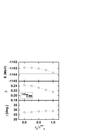
Figure 2: The total energy, deformation parameters $\beta$ and $\gamma$ as functions of the proton pairing reduction factor in ¹⁴⁵Tm calculated by the triaxial RMF approach with PK1, where a reduction factor $f=\Delta_{p}/\Delta^{\rm est.}_{p}$ varying from 0 to 1 has been used in the BCS approximation and the data is given by a grey line.

The total energy, deformation parameters $\beta$ and $\gamma$ in ¹⁴⁵Tm as functions of the pairing reduction factor $f$ are investigated in the triaxial RMF+BCS/PK1 approach and plotted in Fig. 2, in which the total experimental energy for ¹⁴⁵Tm is obtained from the systematic estimated atomic binding energy in Ref. Audi03 by subtracting the electron binding energy according to Ref. Lunney03 .

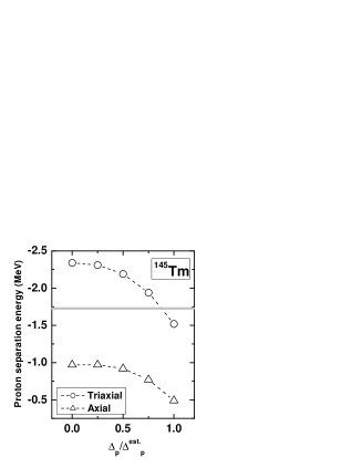
Figure 3: One proton separation energy plotted as a function of proton pairing reduction factor varying from 0 to 1 for ¹⁴⁵Tm in the axial and triaxial RMF calculations with PK1, and pairing correlations treated by the BCS approximation. The neutron pairing gaps for ¹⁴⁵Tm and ¹⁴⁴Er as well as the proton pairing gap for ¹⁴⁴Er are chosen as the estimated values. The data is given by a grey line.

It shows that the proton pairing gap $\Delta_{p}$ has a significant influence on the total energy, but a negligible influence on the predicted deformation parameters. Especially the triaxility parameter $\gamma$ is almost independent on $\Delta_{p}$. The one proton separation energy $S_{p}$ in ¹⁴⁵Tm as a function of the $f$ is plotted in Fig. 3. It is noticed that the $S_{p}$ in the triaxial RMF+BCS/PK1 calculation coincides with the experimental value, $1.728(10)$ MeV Batchelder98 with a certain $\Delta_{p}$ (i.e., $f\simeq 0.9$). However, the axial RMF+BCS/PK1 calculation can not reproduce the experimental data of $S_{p}$. It indicates the importance of both the $\gamma$ degree of deformation and pairing correlations in the description of proton emission in ¹⁴⁵Tm.

The one proton separation energy $S_{p}$, charge radius $r_{c}$, neutron radius $r_{n}$, as well as deformation parameters $\beta$ and $\gamma$, the single-particle orbital occupied by the odd valence proton, and the corresponding spectroscopic factor $u^{2}_{k}$ for ¹⁴⁵Tm are calculated in the axially deformed and triaxial RMF+BCS/PK1 approaches ( $f=0.9$ for proton in ¹⁴⁵Tm). The spectroscopic factor $S_{k}$ of the deformed odd-proton orbital $k$ is approximately given by the unoccupied probability $u^{2}_{k}$ of state $k$ in the daughter nucleus with an even proton number Lalazissis99 . The results are compared with those of relativistic Hartree-Bogoliubov (RHB), the Hartree-Fock-Bogoliubov (HFB-14), the finite-range droplet mass model (FRDM) as well as the experimental data in Table 1. Similar to the HFB-14 prediction, the axially deformed RMF approach predicts an oblate shape with $\beta=-0.21$ for ¹⁴⁵Tm, while the RHB shows a prolate ground-state. The different predicted shapes for ¹⁴⁵Tm can be ascribed to the shape coexistence Geng04 . While the large difference for one proton separation energy between the axially deformed RMF+BCS/PK1($S_{p}=0.62$ MeV) and the RHB calculation ($S_{p}=1.43$ MeV) is ascribed to the treatment of the pairing.

After taking into account the $\gamma$ degree of deformation self-consistently, the one proton separation energy ($S_{p}=1.71$ MeV) in the triaxial RMF+BCS/PK1 calculation is in good agreement with the data. The corresponding deformation parameters are respectively $\beta=0.22$ and $\gamma=28.98^{\circ}$ as shown in Table 1. Furthermore, the spectroscopic factor of the odd valence proton is 0.67, which is consistent with the value 0.51(16) obtained with the WKB approximation calculation Batchelder98 .

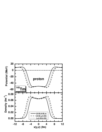
Figure 4: The mean-field potential and density distribution for the protons plotted as functions of $x$ (for $y=0.52$ fm and $z=0.52$ fm) (dotted line), $y$ (for $x=0.52$ fm and $z=0.52$ fm) (dashed line), as well as $z$ (for $x=0.52$ fm and $y=0.52$ fm) (solid line) in ¹⁴⁵Tm.

The triaxiality can make the proton tunneling through the Coulomb barrier easier. The mean-field potential and density distribution of protons in ¹⁴⁵Tm are plotted in Fig. 4 as functions of $x$ (for $y=0.52$ fm and $z=0.52$ fm) (dotted line), $y$ (for $x=0.52$ fm and $z=0.52$ fm) (dashed line), as well as $z$ (for $x=0.52$ fm and $y=0.52$ fm) (solid line), respectively. It shows that both the potential and density distribution are triaxially deformed. The Coulomb barrier is different in different directions and obviously the Coulomb barrier in the direction $y$ is lower than those in $x$ and $z$.

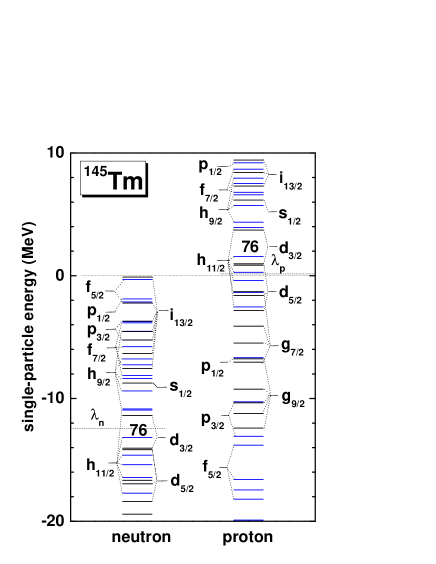
Figure 5: (Color online) Single-particle levels for neutrons and protons in ¹⁴⁵Tm in the triaxial RMF calculation with PK1, and pairing correlations treated by the BCS approximation. The level is labeled with the quantum numbers of its main-component in the spherical Dirac spinor. The black (blue) one is the level with positive (negative) parity.

Apart from the Coulomb barrier, the proton decay probability also depends on its energy and orbital angular momentum, i.e., the centrifugal barrier. In Fig. 5, the single-particle energy levels for both neutron and proton in ¹⁴⁵Tm are given, in which each level is labeled with the quantum numbers of its main-component in the spherical Dirac spinor. The valence proton belongs to the $h_{11/2}$ subshell, which is consistent with the observed spin-parity in Ref. Seweryniak07 .

In refs. Rykaczewski01 ; Karny03 , fine structure in proton emission was observed in ¹⁴⁵Tm. In order to reproduce the experimental partial proton half-lives, it is found that the wave function of the valence proton in ¹⁴⁵Tm is composed mainly of $67\%$ for $0h_{11/2}$ and $3.7\%$ for $1f_{7/2}$, which coupled to the ground state and the excited state of the ¹⁴⁴Er core. Using the particle-core vibration model Hagino01 and assuming deformation $\beta=0.18$, the experimental half-life and the fine structure branching ratio can be reproduced, in which the wave function of the valence proton is composed of $56\%$ for $0h_{11/2}$ and $3\%$ for $1f_{7/2}$ Karny03 . In contrast, by reproducing the fine structure branching, the particle-core vibration calculations in ref. Davids01 give $33\%$ only for $0h_{11/2}$.

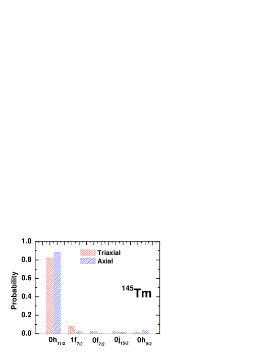
Figure 6: (Color online) Composition of the wave function for the valence proton in ¹⁴⁵Tm calculated with axially and triaxially deformed RMF approaches.

It is interesting to examine the composition of the valence proton in ¹⁴⁵Tm obtained from the present microscopic and self-consistent RMF calculation. In Fig. 6, the main spherical components of wave function for the valence proton in ¹⁴⁵Tm by axially and triaxially deformed RMF calculations are given. The main components in axial RMF calculation are $88.6\%$ for $0h_{11/2}$, $3.7\%$ for $0h_{9/2}$ and $2.3\%$ for $1f_{7/2}$. While in triaxial RMF calculation, the main components are $82.1\%$ for $0h_{11/2}$, $7.9\%$ for $1f_{7/2}$, and $2.3\%$ for $0f_{7/2}$.

The potential and density distribution for the valence proton are obtained in triaxial RMF calculation. To show what the triaxial potentials and proton distribution look like, we plot the potential and density distribution for the valence proton in Fig. 7, in which the potential $V_{k}({\mathbf{r}})$ is given by,

$$V_{k}({\mathbf{r}})=V_{0}({\mathbf{r}})+S({\mathbf{r}})+\frac{(\hbar c)^{2}}{2m_{p}c^{2}}[\sum_{\mu}|F_{k\mu}|^{2}V_{\ell}(r)+\sum_{\mu^{\prime}}|G_{k\mu^{\prime}}|^{2}V_{\ell^{\prime}}(r)],\quad V_{\ell}(r)=\frac{\ell(\ell+1)}{r^{2}},$$ (15)

where $F_{k\mu}$ and $G_{k\mu^{\prime}}$ are respectively the expansion coefficients of the large and small components in spherical basis $|\mu\rangle=|n\ell jm_{j}\rangle$.

A triaxial RMF+BCS/PK1 calculation with the estimated pairing gaps is also carried out for the neighboring proton emitters ¹⁴⁶Tm and ¹⁴⁷Tm. In contrast with the predicted shape transition from prolate to oblate existing from ¹⁴⁵Tm to ¹⁴⁶Tm Moeller95 ; Lalazissis99 , large triaxial deformations have been found for ¹⁴⁶Tm ($\beta=0.19$, $\gamma=39.70^{\circ}$) and ¹⁴⁷Tm ($\beta=0.21$, $\gamma=28.16^{\circ}$). The calculated one proton separation energies are $1.26$ MeV and $0.90$ MeV, which is close to the data, $1.120(10)$ MeV Livingston93 and $1.054(19)$ MeV Sellin93 respectively.

IV Summary

The axially and triaxially deformed RMF approaches have been applied for the description of ground-state properties of the proton emitter ¹⁴⁵Tm with parameter sets PK1 and a constant pairing gap BCS-method for the pairing correlations. It has been found that the triaxiality and pairing correlations are essential to reproduce the one proton separation energy in ¹⁴⁵Tm. The observed spin and parity of the emitted proton can be understood from the main spherical component by the transformation of the quantum number of the valence proton. The corresponding spectroscopic factor in ¹⁴⁵Tm obtained in the present calculation is consistent with that obtained with the WKB approximation calculation. Large triaxial deformations have been found in ¹⁴⁶Tm and ¹⁴⁷Tm as well.

Table 1: Ground-state properties of the proton emitter ¹⁴⁵Tm. The one proton separation energy $S_{p}$, charge radius $r_{c}=\sqrt{r^{2}_{p}+0.64}$, neutron $rms$ radius $r_{n}$, deformation parameters $\beta$ and $\gamma$, as well as the quantum numbers of its main-component in the spherical Dirac spinor $j^{\pi}$ and spectroscopic factor $u^{2}_{k}$ for the valence proton in triaxial RMF calculation with PK1, and pairing correlations treated by the BCS approximation are compared with those of the axial RMF calculation with PK1, and pairing correlations treated by the BCS approximation (Axial), the relativistic Hartree-Bogoliubov calculation (RHB), the Hartree-Fock-Bogoliubov calculation (HFB-14), the finite-range droplet mass model (FRDM) and experimental data. The neutron and proton pairing gaps in ¹⁴⁴Er and ¹⁴⁵Tm are estimated by $\Delta^{\rm est.}_{n}=13.7/\sqrt{A}$ MeV, $\Delta^{\rm est.}_{p}=15.9/\sqrt{A}$ MeV while the proton pairing gap in ¹⁴⁵Tm is given by $0.9\times 15.9/\sqrt{A}$ MeV.

	Sp (MeV)	$r_{c}$ (fm)	$r_{n}$ (fm)	$\beta$	$\gamma$	$j\pi$	$u^{2}_{k}$
Exp. Batchelder98	-1.728					$11/2-$	0.51(16)
Triaxial	-1.71	5.078	4.995	0.22	28.98∘	$11/2-$	0.67
Axial	-0.62	5.073	4.992	-0.21		$7/2-$[523]	0.53
RHB Lalazissis99	-1.43			0.23		$7/2-$[523]	0.47
HFB-14 Goriely07	-1.43	5.073		-0.20
FRDM Moeller95	-1.01			0.25		$1/2+$

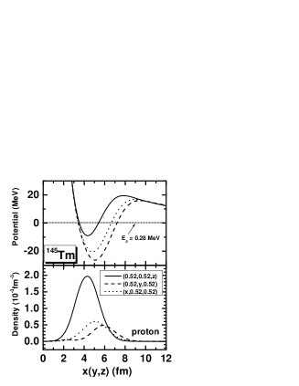
Figure 7: The proton-nucleus potential (upper panel) and density distribution of the valence proton (lower panel) plotted as functions of $x$ (for $y=0.52$ fm and $z=0.52$ fm) (dotted line), $y$ (for $x=0.52$ fm and $z=0.52$ fm) (dashed line), as well as $z$ (for $x=0.52$ fm and $y=0.52$ fm) (solid line) in triaxial RMF calculation with PK1 and pairing correlations treated by BCS approximation. The proton Fermi level is given by the short-dotted line (upper panel).