Can the dynamics of an atomic glass-forming system be described as a continuous time random walk?

Abstract

We show that the dynamics of supercooled liquids, analyzed from computer simulations of the binary mixture Lennard-Jones system, can be described in terms of a continuous time random walk (CTRW). The required discretization comes from mapping the dynamics on transitions between metabasins. This comparison involves verifying the conditions of the CTRW as well as a quantitative test of the predictions. In particular it is possible to express the wave vector-dependence of the relaxation time as well as the degree of non-exponentiality in terms of the first three moments of the waiting time distribution.

The dynamics of supercooled liquids is a very complex process with many non-trivial features such as non-exponential relaxation, decoupling of diffusion and relaxation, significant correlated forward-backward processes (e.g. cage effect), and increasing length scales of relaxation, just to mention some of the most prominent Ediger (1996); P. G. Debenedetti and F. H. Stillinger (2001); Dyre (2006). The complexity of the dynamics originates from the highly cooperative nature of the dynamical processes.

Several phenomenological models have been proposed which attempt to describe the dynamics of supercooled liquids in relatively simple terms, thereby implying some kind of coarse-graining to get rid of the microscopic details of the dynamics. In the free-energy energy Brawer (1984); Dyre (1987); Monthus and Bouchaud (1996); Diezemann et al. (1998) and the RFOT models Xia and Wolynes (2001) the system relaxes, possibly in a multi-step process, between different states. One prominent example is the trap model Dyre (1987); Monthus and Bouchaud (1996), postulating a sequence of escape processes where the waiting time $\tau$ in a configuration is fully governed by its energy and the new configuration is randomly chosen from the set of all possible configurations. Thus, the dynamics is fully described by the waiting time distribution $\varphi(\tau)$. Extending this model by the spatial aspects of the relaxation processes one would, it its simplest version, end up with a continuous-time random walk (CTRW). Note that in general continuous-time random walks (CTRWs) Montroll and Weiss (1965); Monthus and Bouchaud (1996); Odagaki et al. (1994); Barkai and Cheng (2003) as well as the related Levy walks Fogedby (1994); Sokolov (2000) are often used to describe anomalous dynamic properties, characterized by non-trivial power-law behavior of quantities such as the mean-square displacement.

In recent years the facilitated spin models have been revitalized to grasp the dynamics of supercooled liquids Fredrickson and Andersen (1984); Garrahan and Chandler (2002); Berthier and Garrahan (2003); Jung et al. (2004). They are thought to reflect the heterogeneous mobility field of molecular glass-forming systems. One spin corresponds to a small volume which is either unjammed or jammed (spin up or down). The ability of a spin to flip is exclusively governed by the orientation of the adjacent spins. Self-diffusion has been introduced by postulating a random walk of the particle with the chance to move if the old as well as the new site is mobile Jung et al. (2004); Berthier et al. (2005); Jung et al. (2005). This dynamics is also described in terms of a CTRW although for the model variant (East model), supposed to describe fragile systems, a direct mapping is not possible Berthier et al. (2005).

Using the CTRW picture in the context of these phenomenological models does not necessarily imply that it is of relevance for microscopic glass-forming systems. Here we analyze a binary Lennard-Jones system (BMLJ), a standard model of supercooled liquids Kob and Andersen (1995), via computer simulations. The goal of this work is threefold. First, we explicitly show that the required conditions for the applicability of the CTRW approach are fulfilled to a very good approximation. Second, we prove that the CTRW approach not only allows one to obtain the wave-vector dependent relaxation time (as already discussed, e.g., in Berthier et al. (2005)) but also the non-exponentiality of relaxation. Third, the predictions are verified by explicit comparison with the numerical simulations.

We analyze a BMLJ system with N=65 particles at $T=0.5$ which is slightly above the mode-coupling temperature. It has been shown that this system is large enough to recover the diffusion constant without significant finite size effect in the range of temperatures accessible by computer simulations Doliwa and Heuer (2003a, b). Details of the model are described elsewhere Kob and Andersen (1995); Doliwa and Heuer (2003a). The discretization of the dynamics, required for the application of the CTRW approach, results from the use of inherent structures, i.e. local minima of the potential energy landscape Stillinger and Weber (1982, 1984), or the use of metabasins (MBs)Doliwa and Heuer (2003b). Of particular relevance in this work is the incoherent scattering function $S(q,t)=\langle\cos q[x(t+t_{0})-x(t_{0})]\rangle$ where the brackets denote the average over all particles and all $t_{0}$. Furthermore, $x(t)$ is the x-coordinate of a particle. The first decay at short times to a value $f<1$ is due to the fast $\beta$-relaxation whereas the long-time relaxation reflects the $\alpha$-relaxation. It is often described by a KWW function $f\exp[-(t/\tau_{KWW})^{\beta_{KWW}}]$. When analyzing $S(q,t)$ for the sequence of inherent structures rather than actual configurations it turns out at temperatures close to the mode-coupling temperature that the short-time decay disappears and the decay is fully related to the $\alpha$-relaxation with identical values $\tau_{KWW}$, $\beta_{KWW}$ Schrøder et al. (2000). Not surprisingly, the same holds for the sequence of MBs (data not shown). From now on, $S(q,t)$ will represent the case of MBs, thereby describing the $\alpha$-relaxation.

Two important observables enter the CTRW approach: (i) the waiting time distribution $\varphi(\tau)$, (ii) the probability $\pi_{1}(x)$ that a particle during a transition between two MBs moves a specific distance along some fixed direction (here: x). More generally, $\pi_{n}(x)$ expresses the corresponding probability after $n$ MB transitions. The Fourier transform is denoted $\pi_{n}(q)$. Under conditions (C1)-(C3), which form the basis of the CTRW approach and are discussed below, it is possible to express $S(q,t)$ in terms of $\varphi(\tau)$ and $\pi_{1}(q)$.

(C1) $\pi_{1}(x)$ does not depend on the waiting time since the previous transition. From the data in Fig.1 the validity of (C1) directly emerges. Only for the longest waiting times, which only have a very low probability (as reflected by the noise), minor deviations occur. As a consequence the spatial and temporal contributions separate to a very good approximation and one can write

$$S(q,t)=\lim_{N\rightarrow\infty}S_{N}(q,t)=\lim_{N\rightarrow\infty}\sum_{n=0}^{N}S_{n}(t)\pi_{n}(q).$$ (1)

Here $S_{n}(t)$ denotes the probability to have exactly $n$ transitions during time $t$ . This is the central equation of the CTRW because it expresses the total dynamics during time $t$ in terms of discrete processes with well-defined probabilities.

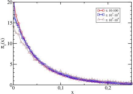
Figure 1: $\pi_{1}(x)$ for different values of the waiting times before the corresponding MB transition. Within statistical uncertainty $\pi_{1}(x)$ does not depend on the waiting time.

(C2) Successive waiting times are statistically uncorrelated so that the time evolution can be regarded as a sequence of randomly chosen waiting times. This has been already shown in Ref.Heuer et al. (2005). Therefore $S_{n}(t)$ can be expressed in terms of the waiting time distribution $\varphi(\tau)$ Berthier et al. (2005); Heuer (2008) (see Eq.8 below). Using the numerically determined $\varphi(\tau)$ and $\pi_{n}(q)$, one can compare $S(q_{max},t)$, obtained from simulation, with the estimation Eq.1 where $q_{max}$ is the maximum of the structure factor; see Fig.2. The agreement is very good except for minor deviations for very long times. Of the order of $10^{2}$ MB transition processes are required to have complete relaxation.

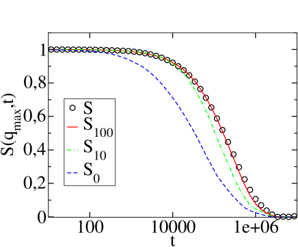
Figure 2: Comparison of the actual incoherent scattering function $S(q_{max},t)$ with the estimated function $S_{N}(q_{max},t)$ for different values of $N$.

(C3) Subsequent transitions are spatially uncorrelated. The underlying Markov hypothesis can be formally written as

$$\pi_{n}(x)=\int dx^{\prime}\pi_{n-1}(x^{\prime})\pi_{1}(x-x^{\prime}).$$ (2)

In Fourier-space this convolution reads

$$\pi_{n}(q)=\pi_{1}(q)^{n}.$$ (3)

From the analysis of the mean square displacement (MSD) in Ref.Doliwa and Heuer (2003a) it became clear that there exist minor forward-backward correlations for the MB transitions so that (C3) cannot hold in a strict sense. However, due to the expected locality of forward-backward transitions one may expect that for longer length scales, i.e. smaller $q$, they become irrelevant. Indeed, one has a well-defined limit $a^{2}\equiv\lim_{n\rightarrow\infty}(1/n)\langle x^{2}\rangle_{\pi_{n}}=0.005$ which is slightly smaller than $\langle x^{2}\rangle_{\pi_{1}}=0.009$ Doliwa and Heuer (2003a) where $\langle x^{2}\rangle_{f}\equiv\int\,dx\,x^{2}f(x)$. To check this in detail, we have analyzed the n-dependence of $\pi_{n}(q)$, shown in Fig.3 for different values of the wave-vector $q$. Interestingly, for $q=q_{max}$ the limiting behavior $\pi(q)\equiv(\pi_{n}(q))^{1/n}=const$ is already reached for $n\geq 5$, as reflected by the straight line. For smaller $q$-values Eq.3 holds even better. Since in the range of relevant $q$ values one has $a^{2}q^{2}\ll 1$ the term $\pi(q)$ can be approximated by $1-q^{2}a^{2}/2$. Using inherent structures rather than MBs the large-n regime would be only reached for $n\approx 10^{3}$ Doliwa and Heuer (2003a). This would strongly invalidate (C3).

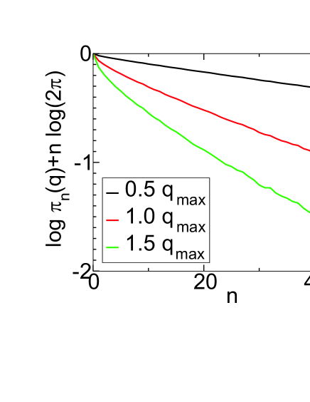
Figure 3: The $n$-dependence of $\pi_{n}(q)$ for different values of $q$.

Using (C1)-(C3), and substituting all $\pi_{n}(q)$ by $\pi(q)$, the temporal Laplace transform of the incoherent scattering function, i.e. $S(q,\lambda)$, can be calculated analytically, yielding the Montroll-Weiss equation Montroll and Weiss (1965). Unfortunately, the inverse Laplace transform of $S(q,\lambda)$ cannot be analytically performed to calculate $S(q,t)$. Therefore we proceed in a somewhat different way. First, we define

$$\tau_{0}(q)\equiv\int dtS(q,t)$$ (4)

and

$${\beta}_{m}(q)\equiv\frac{\tau_{0}^{2}(q)}{\int dt\,t\,S(q,t)}.$$ (5)

$\tau_{0}(q)$ denotes the relaxation time at wave vector $q$ and ${\beta}_{m}$ reflects the shape of $S(q,t)$, based on the different moments. Whereas for exponential relaxation one has ${\beta}_{m}=1$ it decreases when $S(q,t)$ decays in a non-exponential manner. In case of KWW relaxation one has ${\beta}_{m}=\Gamma^{2}(1/\beta_{KWW})/(\beta_{KWW}\Gamma(2/\beta_{KWW}))$ where $\Gamma()$ denotes the $\Gamma$-function (e.g. $\beta_{KWW}=1/2$ corresponds to ${\beta}_{m}=1/3$). ${\beta}_{m}$ depends monotonously on $\beta_{KWW}$ . Thus, ${\beta}_{m}$ is a measure of the degree of non-exponentiality.

Our goal is to find simple expressions for $\tau_{0}(q)$ and ${\beta}_{m}(q)$. For this purpose one can introduce the persistence time distribution $\xi(\tau)$. It denotes the probability that for a random starting point in time the next transition occurs a time $\tau$ later Montroll and Weiss (1965); Jung et al. (2005). It is related to the waiting time distribution via

$$\xi(\tau)=\int_{\tau}^{\infty}dt^{\prime}\varphi(t^{\prime})/\langle\tau\rangle_{\varphi}.$$ (6)

Furthermore, it is related to $S_{0}(t)$ via

$$S_{0}(t)=\int_{t}^{\infty}\,dt^{\prime}\xi(t^{\prime}).$$ (7)

For $n>0$ the Laplace-transform of $S_{n}(t)$ is given by

$$S_{n}(\lambda)=\xi(\lambda)^{2}\varphi(\lambda)^{n-1}/\langle\tau\rangle_{\varphi}.$$ (8)

Straightforward calculation yields $\int\,dt\,S_{n}(t)=S_{n}(\lambda=0)=\langle\tau\rangle_{\varphi}$ for $n>0$. Note that for two functions, connected by $f(t)=\int_{t}^{\infty}dt^{\prime}g(t^{\prime})$, one obtains

$$\langle t^{n}\rangle_{f}=\frac{\langle t^{n+1}\rangle_{g}}{n+1}.$$ (9)

This implies $\int\,dt\,S_{0}(t)=\langle\tau\rangle_{\xi}$, i.e. the average persistence time. Using again Eq.9 it can be also expressed as $\langle\tau^{2}\rangle_{\varphi}/\langle\tau\rangle_{\varphi}$. Note that $\langle\tau\rangle_{\xi}/\langle\tau\rangle_{\varphi}\gg 1$ for a broad waiting time distribution, reflecting large dynamic heterogeneities. Equivalently, this means that the time until the first transition after a randomly chosen time takes much longer than the typical time $\langle\tau\rangle_{\varphi}$ between successive jumps.

Using Eq.1 together with Eqs.3 and 9 one obtains Berthier et al. (2005)

$$\tau_{0}(q)/\langle\tau\rangle_{\varphi}=\frac{\langle\tau\rangle_{\xi}}{\langle\tau\rangle_{\varphi}}+\frac{\pi_{1}(q)}{1-\pi_{1}(q)}\approx\frac{\langle\tau\rangle_{\xi}}{\langle\tau\rangle_{\varphi}}+\frac{2}{q^{2}a^{2}}.$$ (10)

We note in passing that $\langle\tau\rangle_{\xi}$ can be identified with the structural relaxation time $\tau_{\alpha}$ Berthier et al. (2005). To determine the simulated $\tau_{0}(q)$ via integration over $S(q,t)$ we have first fitted $S(q,t)$ by a sum of two stretched exponentials and then performed the integration analytically.

In Fig.4a we show the comparison with the simulated data. We have used $\langle\tau\rangle_{\xi}/\langle\tau\rangle_{\varphi}=27$, as determined from the numerically determined waiting time distribution. The $q$-dependence of $\tau_{0}(q)$ is qualitatively similar to the data reported in Berthier (2004) and Stariolo and Fabricius (2006). Note, however, that with the present definition of $\tau_{0}(q)$ and the reference to the MB dynamics for the definition of $\varphi(\tau)$ and $a^{2}$ a parameter-free prediction of the $q$-dependence becomes possible. At large $q$ ($q>q_{max}$) the system relaxes somewhat faster because the effective value of $a^{2}$ increases due to the relevance of forward-backward correlations (see above). For smaller $q$, given by $1/q^{2}\approx\langle\tau\rangle_{\xi}/\langle\tau\rangle_{\varphi}a^{2}/2$, there is a crossover of $\tau_{0}(q)$ from the q-independent large-q limit to the small-q limit $\tau_{0}(q)=2\langle\tau\rangle_{\varphi}/(q^{2}a^{2})$. Thus, for large dynamic heterogeneities, i.e. low temperatures, this crossover may happen at quite large distances Berthier et al. (2005). Similarly, these non-trivial features are also reflected by a specific time evolution of the self-part of the van Hove function $G_{s}(x,t)$ Chaudhuri et al. (2007). The deviations of $G_{s}(x,t)$ from simple diffusion have been analysed in detail in Szamel and Flenner (2006).

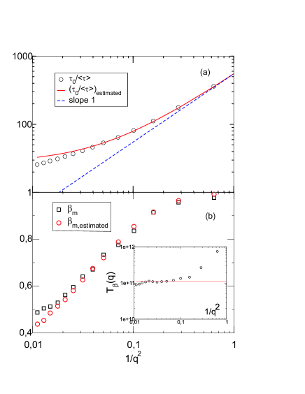
Figure 4: The $q$-dependence of (a) $\tau_{0}(q)$ together with its estimation via Eq.10 and (b) of ${\beta}_{m}(q)$ together with its estimation. In the inset the validity of the theoretical expectation $(d/dq)T_{\beta}(q)=0$ is tested.

For the discussion of ${\beta}_{m}(q)$ we first rewrite Eq.5 as

$${\beta}_{m}^{-1}(q)-1=T_{\beta}(q)/\tau_{0}^{2}(q)$$ (11)

with $T_{\beta}(q)=\int\,dt\,t\,S(q,t)-\tau_{0}^{2}(q)$. Following the standard derivation of the Montroll-Weiss equation one can show after a tedious but straightforward calculation with the ingredients, presented in this work, that $(d/dq)T_{\beta}(q)=0$ Heuer (2008), i.e. $T_{\beta}(q)\equiv T_{\beta}$. For the evaluation of $T_{\beta}$ we choose the limit $q\rightarrow\infty$ where $S(q,t)=S_{0}(t)$. Following Eq.9 the first term equals $\langle\tau^{2}\rangle_{\xi}/2$ whereas the second term is given by $\langle\tau\rangle_{\xi}^{2}$, i.e.

$$T_{\beta}(q)=\frac{\langle\tau^{2}\rangle_{\xi}}{2}-\langle\tau\rangle_{\xi}^{2}$$ (12)

which directly reflects the width of the persistence time distribution. Note that via Eq.9 $T_{\beta}$ involves the third moment of the waiting time distribution $\varphi(\tau)$. Interestingly, the q-dependence of ${\beta}_{m}(q)$ is fully governed by $\tau_{0}(q)$. Thus, the degree of non-exponentiality displays exactly the same crossover-behavior as the relaxation time. A comparison of Eqs.11 and 12 with the numerical data is shown in Fig.4b, showing again a good agreement. Actually, due the extreme dependence of the third moment on the fine details of the long-time behavior of $\varphi(\tau)$ a precise estimation of $T_{\beta}$ from $\varphi(\tau)$ is not possible. Again, the deviations at large $q$ reflect the more complicated dynamics at short length-scales. The deviations for small $q$ come from the trivial fact that $T_{\beta}(q)$ results from a difference of two very large numbers which, because of the nearly-exponential behavior, are very similar.

In summary, the present work has shown that the CTRW approach, more or less explicitly used in different models of the glass transition, can indeed be numerically derived for an atomic glass-forming system. This shows that after an appropriate coarse-graining procedure (here: the metabasins) the complex dynamics of supercooled liquids becomes relatively simple. Note that on a lower level of coarse-graining, namely the inherent structures, (C3) and thus the CTRW approach is strongly violated. In contrast, more coarse-graining, e.g. by joining some successive MBs, would start to change $S(q,t)$ by rendering it more exponential. In analogy to the previous model considerations the CTRW approach is formulated for a subsystem of a large macroscopic system (one cooperatively rearranging region, one probe molecule, here: a small system with periodic boundary conditions). Generalization to large systems, thereby keeping information about possible correlations and predicting multi-point correlation functions, is a challenge for the future.

We gratefully acknowledge the support by the DFG via SFB 458 and helpful discussions with L. Berthier.

References

- Ediger (1996) M. D. Ediger, J. Phys. Chem. 100, 13200 (1996).
- P. G. Debenedetti and F. H. Stillinger (2001) P. G. Debenedetti and F. H. Stillinger, Nature 410, 259 (2001).
- Dyre (2006) J. Dyre, Rev. Mod. Phys. 78, 953 (2006).
- Brawer (1984) S. Brawer, J. Chem. Phys. 81, 954 (1984).
- Dyre (1987) J. Dyre, Phys. Rev. Lett. 58, 792 (1987).
- Monthus and Bouchaud (1996) C. Monthus and J. P. Bouchaud, J. Phys. A-Math. Gen. 29, 3847 (1996).
- Diezemann et al. (1998) G. Diezemann, H. Sillescu, G. Hinze, and R. Bohmer, Phys. Rev. E 57, 4398 (1998).
- Xia and Wolynes (2001) X. Xia and P. G. Wolynes, Phys. Rev. Lett. 86, 5526 (2001).
- Montroll and Weiss (1965) E. Montroll and G. Weiss, J. Math. Phys. 6, 167 (1965).
- Odagaki et al. (1994) T. Odagaki, J. Matsui, and Y. Hiwatari, Physica A 204, 464 (1994).
- Barkai and Cheng (2003) E. Barkai and Y.-C. Cheng, J. Chem. Phys. 118, 6167 (2003).
- Fogedby (1994) H. C. Fogedby, Phys. Rev. E 50, 1657 (1994).
- Sokolov (2000) I. M. Sokolov, Phys. Rev. E 63, 011104 (2000).
- Fredrickson and Andersen (1984) G. Fredrickson and H. Andersen, Phys. Rev. Lett. 53, 1244 (1984).
- Garrahan and Chandler (2002) J. P. Garrahan and D. Chandler, Phys. Rev. Lett. 89, 035704 (2002).
- Berthier and Garrahan (2003) L. Berthier and J. P. Garrahan, Phys. Rev. E. 68, 041201 (2003).
- Jung et al. (2004) Y. Jung, J. Garrahan, and D. Chandler, Phys. Rev. E 69, 061205 (2004).
- Berthier et al. (2005) L. Berthier, D. Chandler, and J. Garrahan, Europhys. Lett. 69, 320 (2005).
- Jung et al. (2005) Y. Jung, J. Garrahan, and D. Chandler, J. Chem. Phys. 123, 084509 (2005).
- Kob and Andersen (1995) W. Kob and H. C. Andersen, Phys. Rev. E 52, 4134 (1995).
- Doliwa and Heuer (2003a) B. Doliwa and A. Heuer, Phys. Rev. E 67, 030501 (2003a).
- Doliwa and Heuer (2003b) B. Doliwa and A. Heuer, Phys. Rev. E 67, 031506 (2003b).
- Stillinger and Weber (1982) F. H. Stillinger and T. A. Weber, Phys. Rev. A 25, 978 (1982).
- Stillinger and Weber (1984) F. H. Stillinger and T. A. Weber, Science 225, 983 (1984).
- Schrøder et al. (2000) T. B. Schrøder, S. Sastry, J. C. Dyre, and S. C. Glotzer, J. Chem. Phys. 112, 9834 (2000).
- Heuer et al. (2005) A. Heuer, B. Doliwa, and A. Saksaengwijit, Phys. Rev. E 72, 021503 (2005).
- Heuer (2008) A. Heuer, (submitted) (2008).
- Berthier (2004) L. Berthier, Phys. Rev. E 69, 020201 (2004).
- Stariolo and Fabricius (2006) D. A. Stariolo and G. Fabricius, J. Chem. Phys. 125, 064505 (2006).
- Chaudhuri et al. (2007) P. Chaudhuri, L. Berthier, and W. Kob, cond-mat: 07072095 (2007).
- Szamel and Flenner (2006) G. Szamel and E. Flenner, Phys. Rev. E 73, 011504 (2006).