Properties of ideal Gaussian glass-forming systems

Abstract

We introduce the ideal Gaussian glass-forming system as a model to describe the thermodynamics and dynamics of supercooled liquids on a local scale in terms of the properties of the potential energy landscape (PEL). The first ingredient is the Gaussian distribution of inherent structures, the second a specific relation between energy and mobility. This model is compatible with general considerations as well as with several computer simulations on atomic computer glass-formers. Important observables such as diffusion constants, structural relaxation times and kinetic as well as thermodynamic fragilities can be calculated analytically. In this way it becomes possible to identify a relevant PEL parameter determining the kinetic fragility. Several experimental observations can be reproduced. The remaining discrepancies to the experiment can be qualitatively traced back to the difference between small and large systems.

I Introduction

The understanding of the dynamics of supercooled liquids is still far from being complete P. G. Debenedetti and F. H. Stillinger (2001); Binder and Kob (2005); Dyre (2006); Lubchenko and Wolyness (2006). A lot of insight has been gained from simulations . For example, in real space the microscopic nature of dynamic heterogeneities has been clarified Hurley and Harrowell (1995); Kob et al. (1997); Donati et al. (1998, 1999a, 1999b); Heuer and Okun (1997); Qian et al. (1999). Using the framework of the potential energy landscape (PEL) a lot of insight could be also gained in configuration space Wales (2003); Sciortino (2005). A key aspect is the use of inherent structures (IS) , i.e. local minima of the PEL. Upon minimization basically all configurations can be mapped on a IS. In this way the regular dynamics can be mapped on a hopping dynamics between IS Stillinger and Weber (1982, 1984). Physically, this mapping can be interpreted as a removal of the vibrational degrees of freedom. However, as explicitly shown in Schrøder et al. (2000) the properties of the structural relaxation remain identical for sufficiently low temperatures. Generally speaking, the mapping on the IS can be interpreted as a coarse-graining procedure. At low temperatures the IS dynamics displays many correlated forward-backward jumps between adjacent IS. In a further coarse-graining step it is possible to define metabasins (MB) by an appropriate merging of adjacent IS F. H. Stillinger (1995); Middleton and Wales (2001); Doliwa and Heuer (2003a, b); Denny et al. (2003). In this way the effect of correlated forward-backward motion has basically disappeared.

A key question deals with the relation between thermodynamics and dynamics. For example the empirical Adam-Gibbs relation Adam and Gibbs (1965)

$$\Gamma(T)=\Gamma_{0}\exp(-B_{AG}/Ts_{c}(T))$$ (1)

relates the configurational entropy $s_{c}$ to the local relaxation rate $\Gamma$. A further relation between thermodynamics and dynamics is formulated via the fragilities. In the spirit of the thermodynamic fragility as discussed in Martinez and Angell (2001); Wang et al. (2006) one can define the thermodynamic fragility index via G. Ruocco, F. Sciortino, F. Zamponi, C. De Micheleand T. Scopigno (2004)

$$m_{thermo}=-\beta_{g}\frac{S_{c}^{\prime}(\beta_{g})}{S_{c}(\beta_{g})}.$$ (2)

where $T_{g}=1/\beta_{g}$ (choosing $k_{B}=1$) denotes the glass-transition temperature. Furthermore, the kinetic fragility is defined as

$$m_{kin}=d\ln\tau_{\alpha}/d(T_{g}/T).$$ (3)

Qualitatively, it denotes the slope of the relaxation time (or viscosity) in the Angell-plot Angell (2000); Martinez and Angell (2001). Empirically, one finds a significant correlation between the kinetic and the thermodynamic fragility Martinez and Angell (2001). In principle the kinetic fragility may also be defined for the diffusion constant. Due to the violation of the Stokes-Einstein relation Fujara et al. (1992) minor variations of the value of $m_{kin}$ will be present. Furthermore, it turns out that for the set of all glass-forming systems one observes a significant correlation between $m_{kin}$ and the degree of non-exponentiality, expressed, e.g., by the exponent $\beta_{KWW}$ of the stretched exponential function Bohmer et al. (1993). If one restricts oneself, however, to the set of all molecular glass-forming systems (excluding in particular network forming systems and polymers) the residual correlation is very weak (-0.28) and the values of $\beta_{KWW}$ are restricted for most of the systems ($>80\%$) in that work to a relatively small regime between 0.5 and 0.62 Bohmer et al. (1993); Heuer (2008). In contrast, the network-forming systems are characterized by nearly exponential relaxation and small values of $m_{kin}$.

In the language of the IS or the MB the thermodynamic properties at constant volume are to large extent determined by their energy distribution $G(e)$. For many systems it has been shown numerically that the distribution of IS can be described by a Gaussian Sciortino et al. (1999a); Buechner and Heuer (1999); Starr et al. (2001); Nave et al. (2000). Even for BKS-SiO₂ the distribution is Gaussian, albeit displaying a low-energy cutoff in the range of accessible temperatures for computer simulations Saksaengwijit et al. (2004). Furthermore, it turns out that the distribution of IS and MB is nearly identical in the relevant regime of low-energy states Doliwa and Heuer (2003b).

Within the PEL approach it is possible to relate the thermodynamic and the dynamic aspects Doliwa and Heuer (2003a, b); Denny et al. (2003); Doliwa and Heuer (2003c). This is based on the observation that the escape rate from a MB can be expressed in terms of its energy, i.e. $\Gamma(e,T)$. Furthermore, it turns out that the temperature dependence of the diffusion constant $D(T)$ can be fully expressed in terms of the average local escape rate. As a consequence, knowledge of $G(e)$ and $\Gamma(e,T)$ allows one to predict $D(T)$. A similar type of relation between energy and mobility can be found, e.g., for the trap model Monthus and Bouchaud (1996).

The goal of this work is to elucidate the properties of a system with a Gaussian distribution $G(e)$ of MB. The functional form of $\Gamma(e,T)$ is rationalized by different models, discussed in literature, and at the same time by comparison with previous computer simulations on the binary mixture Lennard-Jones system (BMLJ) and silica (BKS-SiO₂). On this basis we define an ideal Gaussian glass-former (IGGF). For the IGGF several observables can be determined analytically such as the temperature dependent diffusion constant and relaxation time, its kinetic and thermodynamic fragility and its non-exponentiality. In this way it becomes possible, e.g., to elucidate the relevant PEL parameters which determine the fragility. In Sect.II the IGGS is introduced and in Sect.III its main properties are calculated. We end with a critical discussion and a summary in Sect.IV.

II Description of the ideal Gaussian glass-former

II.1 Thermodynamics

Of crucial importance for the properties of a glass-forming system is the number density of IS, denoted $G(e)$. Here we always consider a system with $N$ particles. For many different systems, studied via computer simulations, a Gaussian density of IS has been found Starr et al. (2001); Nave et al. (2000); Sciortino et al. (1999b); Buechner and Heuer (2000), i.e.

$$G(e)=\exp(\alpha N)\frac{1}{\sqrt{2\pi\sigma^{2}}}\exp(-(e-e_{0})^{2}/2\sigma^{2}).$$ (4)

A notable exception is BKS-SiO₂. This system is characterized by a low-energy cutoff Saksaengwijit and Heuer (2006a) which gives rise to the fragile-to-strong crossover Saika-Voivod et al. (2004); Saksaengwijit and Heuer (2006a). In principle, for the calculations, shown below, the effect of a low-energy cutoff can be incorporated Heuer (2008). Here we mainly concentrate just on the case of a purely Gaussian density of IS.

For a closer discussion one has to take into account that the average curvature around the minima may depend on $e$. For different systems it turns out to a very good approximation that one has a linear energy-dependence for the free energy $F_{harm}(e)$, related to the harmonic vibration in a well Sciortino et al. (1999a); Buechner and Heuer (1999); Sastry (2001); Starr et al. (2001); Mossa et al. (2002); Giovambattista et al. (2003); Sciortino et al. (2003). This can be written as

$$F_{harm}(e)=const-\beta_{harm}e.$$ (5)

The constant $\beta_{harm}$ is a material constant. The meaning of the sign of $\beta_{harm}$ is visualized in Fig.1.

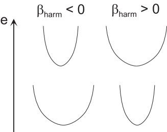
Figure 1: A sketch of the cases $\beta_{harm}<0$ and $\beta_{harm}>0$. Shown are typical curvatures around representative IS at different energies.

The Boltzmann distribution $p_{eq}(e)$ describes the probability to be (at a randomly chosen time) in an IS with energy $e$. $p_{eq}(e)$ is proportional to $G(e)\exp(-\beta e)$ when $\beta_{harm}=0$. Taking into account the curvature-effect, introduced above, one finds

$$p_{eq}(e)\propto G_{eff}(e)\exp(-\beta e)$$ (6)

with the effective density

$$G_{eff}(e)\propto G(e)\exp(-F_{harm}(e))\propto\exp(-(e-e_{0,eff})^{2}/2\sigma^{2}).$$ (7)

and $e_{0,eff}=e_{0}+\beta_{harm}\sigma^{2}$. Thus the presence of an energy-dependent average curvature can be incorporated by a shift of the Gaussian distribution of states.

The standard definition of the configurational entropy is $-\sum_{i}p_{i}\ln p_{i}$ where the sum is over all states (not energies). Mapping this relation to the description in terms of energies one obtains

$$S_{c}(T)=\int dep_{eq}(e)\ln(G(e)/p_{eq}(e))=\int dep_{eq}(e)S_{c}(e)-\int dep_{eq}(e)\ln p_{eq}(e).$$ (8)

For the $G(e)$ and $p_{eq}(e)$, obtained for the Gaussian distribution, one obtains from the first term

$$S_{c}(T)=N\alpha-(1/2)\sigma^{2}\left(\beta-\beta_{harm}\right)^{2}.$$ (9)

For large $N$ one expects that $\sigma^{2}\propto N$ due to the central limit theorem. Then $S_{c}(T)$ becomes extensive as expected. In contrast, the last term in Eq.8, which would give rise to $1/2$, can be neglected because it is not extensive and just gives rise to a minor redefinition of $\alpha$ ($\alpha\rightarrow\alpha+1/2N$).

Defining the Kauzmann-temperature by the condition $S_{c}(T_{K})=0$ (and $\beta_{K}=1/T_{K}$) Eq.9 can be equivalently expressed as

$$TS_{c}(T)=[(N\alpha)+\sigma^{2}\beta\beta_{K}/2-\sigma^{2}\beta_{harm}^{2}/2](T-T_{K}).$$ (10)

Neglecting the temperature-dependence of the second term this is actually the standard expression when deriving the VFT-temperature dependence (e.g. $\ln(D(T)/D_{0})\propto 1/(T-T_{0})$ where often $T_{0}\approx T_{K}$ is found) from the Adam-Gibbs expression Sastry (2001). Using a similar way of rewriting the configurational entropy, this type of argument can be already found in Sastry (2001). In any event, for the further analysis we will use the expression Eq.9 due to its simplicity.

II.2 Transitions between MB: Models

There is a long history of models which describe the dynamics in configuration space on a phenomenological level Brawer (1984); Dyre (1987); Arkhipov and Baessler (1994); Monthus and Bouchaud (1996); Diezemann (1997); Diezemann et al. (1998). One considers a region of the viscous fluid which can cooperatively rearrange via a transition state. For the time being the initial and final states may be characterized by the energy of the respective IS (or MB). For sufficiently low temperatures the elementary rearrangement process is considered to be activated: the system leaves a state with energy $e$, crosses a high-energy transition state with rate $\Gamma(e)$ (from now on the variable $T$ is omitted) and ends up in a new state which is uncorrelated to the initial one. Different names can be found for essentially identical models (e.g. trap model, free energy model) following this scenario.

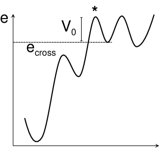
Figure 2: Sketch of the multi-step escape process, including the definition of $V_{0}$. The barrier with the star is supposed to be the critical barrier beyond which $p_{back}<0.5$.

The hopping rate $\Gamma(e)$ is characterized by two energies. $e_{cross}$ denotes the energy of the IS just after the final barrier, which has a height $V_{0}$; see Fig.2 for the sketch. According to the model assumptions $e_{cross}$ and $V_{0}$ are independent of the initial energy $e$. Actually, even in more complex systems like the random energy model one can argue via percolation arguments that $e_{cross}$ is independent of $e$ Dyre (1995). More generally, in a percolation-like picture of the PEL $e_{cross}$ corresponds to the energy level from which on the system finds adjacent states with similar energies and thus does not have to increase further in the PEL for the final relaxation. Defining $E_{app}(e)$ as the apparent activation energy to escape from energy $e$, this scenario can be written as

$$\Gamma(e)=\Gamma_{0}(e)\exp(-\beta E_{app}(e))$$ (11)

with

$$E_{app}(e)=e_{cross}+V_{0}-e$$ (12)

for $e\leq e_{cross}$ and $E_{app}(e)=V_{0}$ for $e\geq e_{cross}$. Stated differently, the escape for energies lower than $e_{cross}$ is solid-like (activated) whereas otherwise it is liquid-like Doliwa and Heuer (2003c).

The energy-dependent prefactor $\Gamma_{0}(e)$ reflects possible entropic effects. As argued in Brawer (1984, 1985) the prefactor $\Gamma_{0}(e)$ contains an energy-dependent factor $M_{entro}$ which denotes the number of escape paths to reach a high-energy state with energy $e_{cross}$. In most models this is neglected by simply choosing $\Gamma_{0}(e)=\Gamma_{0}$. This would be justified in case of 1D reaction paths or low-dimensional percolation paths. A simple expression for $M_{entro}$ can be formulated if every state with energy $e_{cross}$ can be reached from exactly one state with energy $e(<e_{cross})$. It is given by $M_{entro}=G(e_{cross})/G(e)$ Saksaengwijit and Heuer (2006b), i.e.

$$\Gamma_{0}(e)=\Gamma_{0}G(e_{cross})/G(e).$$ (13)

This holds for $e<e_{cross}$ in the opposite limit one just has $\Gamma_{0}(e)=\Gamma_{0}$. For $e_{cross}-e\ll e_{0}-e_{cross}$ Eq.13 can be approximated as

$$\Gamma_{0}(e)\approx\Gamma_{0}\exp((e_{0}-e_{cross})(e_{cross}-e)/\sigma^{2}).$$ (14)

For later purposes this is rewritten as

$$\Gamma_{0}(e)=\Gamma_{0}\exp(\kappa k_{entro}(e_{cross}-e))$$ (15)

with

$$k_{entro}=(e_{0,eff}-e_{cross})/\sigma^{2}$$ (16)

and

$$\kappa=\frac{e_{0}-e_{cross}}{e_{0,eff}-e_{cross}}$$ (17)

This somewhat complicated way to rewrite Eq.14 is motivated in two ways. First, because $p_{eq}(e)$ is directly related to $G_{eff}(e)$ and thus to $e_{0,eff}$, see Eq.6, it is more convenient to use $e_{0,eff}$ rather than $e_{0}$. Second, in practice the factor $\kappa$ has to be treated as an empirical parameter because the increase of the entropic term $\Gamma_{0}(e)$ with decreasing energy may somewhat deviate from the specific scenario, described above. The relevant energy scales are summarized in Fig.3.

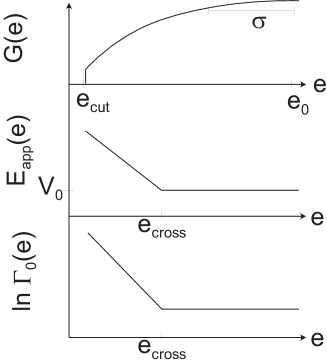
Figure 3: Sketch of the energies, introduced in the text. A possible difference between $G(e)$ and $G_{eff}(e)$ is neglected.

It is convenient to introduce the shifted inverse temperature

$$\tilde{\beta}=\beta-\kappa k_{entro}.$$ (18)

In principle all calculations, shown in this work, can be performed as well for $\kappa\neq 1$. However, since the influence of the entropic prefactor is not as important as the energetic term the additional complexity of the expressions is not worth the additional information for $\kappa\neq 1$. In what follows we therefore always choose $\kappa=1$.

Now one can rewrite Eq.11 as

$$\Gamma(e)=\Gamma_{0}\exp(-\tilde{\beta}(e_{cross}-e))\exp(-\beta V_{0})$$ (19)

and, for a Gaussian density of states,

$$p_{eq}(e)\propto G_{eff}(e)\exp(-\beta e)\propto\exp[-(e-e_{cross}+\sigma^{2}\tilde{\beta})^{2}/2\sigma^{2}].$$ (20)

When comparing Eq. 19 with simulations one has to take into account that the simulated system may contain more than one elementary system. Each subsystem is characterized by an energy $e_{i}$ and $e=\sum e_{i}$. For a superposition of $M$ independent subsystems the total hopping rate $\Gamma_{M}(e)$ is just the sum of the individual hopping rates $\Gamma(e_{i})$. To a first approximation one may assume that the energy $e$ is equally distributed among the $M$ subsystems, yielding $\Gamma_{M}(e)=M\Gamma(e/M)$. A closer analysis shows that apart from another energy-independent factor this is indeed the correct expression Heuer (2008). This expression for $\Gamma_{M}(e)$ suggests to generalize Eq.19 to

$$\Gamma(e)=\Gamma_{0}\exp(-\lambda\tilde{\beta}(e_{cross}-e))\exp(-\beta V_{0})$$ (21)

Here $1/\lambda$ is a measure for the number of elementary subsystems, present in the specific system. This completes the definition of the IGGF. For later purposes we introduce the dimensionless quantity

$$\mu\equiv\tilde{\beta}\sigma$$ (22)

which will turn out to be the central quantity characterizing the properties of the IGGF.

II.3 Comparison with simulations

The above scenario has been compared with simulations of relatively small systems of the BMLJ system $(N=65)$ Doliwa and Heuer (2003b) and BKS-SiO₂ $(N=99)$ Saksaengwijit and Heuer (2006b)). This comparison has been performed for MB in order to have a random-walk type dynamics in configuration space. With IS it would have been impossible to express observables such as the diffusion constant or the relaxation time just in terms of the waiting times Doliwa and Heuer (2003b); Heuer (2008). For the comparison the average waiting time in MB of a given energy $e$ have been determined, denoted as $\langle\tau(e)\rangle$. Naturally, the average escape rate $\Gamma(e)$ is then given by

$$\Gamma(e)=\frac{1}{\langle\tau(e)\rangle}.$$ (23)

Note that this definition does not imply that the escape from a MB with energy $e$ corresponds to an exponential waiting time distribution with average waiting time $\langle\tau(e)\rangle$.

The simulations have fully confirmed the validity of Eq.21 except for a slight smearing out effect for energies close to $e_{cross}$. Actually, the effective barriers could be identified by a closer analysis of the relevant minima and saddles of the PEL Doliwa and Heuer (2003b). Actually, in de Souza and Wales (2006) it has been shown that the additional barrier before the final transition (denoted $V_{0}$ above) and the barrier, governing the local forward-backward motion at low temperatures (within a MB) are roughly the same.

Very recently, de Souza and Wales have analyzed the temperature dependence of the mean square displacement, evaluated for a fixed time $\tau$ de Souza and Wales (2006). Of course, for very large $\tau$ this analysis recovers the standard diffusion coefficient. For ambient $\tau$, which for the lowest temperatures is significantly shorter than $\tau_{\alpha}$, the authors observe a simple Arrhenius behavior with the high-temperature activation energy $V_{0}$. For lower temperatures this approach is sensitive to the local forward-backward motion within a MB. The barriers in this regime are of the order of $V_{0}$ so that the local processes remain activated with the high-temperature activation energy. This strengthens the observation that it is roughly the same value $V_{0}$ which governs the additional barrier height at low and high energies.

Furthermore it turns out that $\Gamma_{0}(e)$ indeed shows an exponential dependence of energy. Interestingly, $\Gamma_{0}(e_{cross})\approx 1/20$ fs^-1 is of the order of typical molecular time scales. This also suggests that the increase below $e_{cross}$ is due to entropic reasons.

The PEL parameters, obtained from the fitting, are listed in Tab.1. Note that if not mentioned otherwise from now on all energies are expressed relative to $e_{0,eff}$, i.e. the maximum of $G_{eff}(e)$. For the analytical calculations, to be presented below, it is convenient to exclusively use Eq.21, i.e. using $e<e_{cross}$ and $\tilde{\beta}>0$. The first relation starts to be very well fulfilled if $e_{cross}-\langle e(T)\rangle>\sigma$ which roughly implies $T<0.6$ in case of BMLJ and $T<3600$ K in case of BKS-SiO₂. In this temperature range one also has $\tilde{\beta}>0$.

		thermodynamic				dynamic
	N	$\sigma$	$-e_{cut}$	$\beta_{harm}$	$\alpha$	$-e_{cross}$	$\lambda$	$\kappa$	$V_{0}$	$\Gamma_{0}$
BKS-SiO2	99	3.5 eV	43.4 eV	$\approx 0$	1.14	37.5 eV	0.66	0.62	0.8 eV	1/(20 fs)
BMLJ	65	3.0	-	-0.3	0.73	12.9	0.55	0.3	1.0	1/150

Table 1: The thermodynamic and dynamic PEL parameters, obtained from simulation of BKS-SiO₂ and BMLJ.

Interestingly, $e_{cross}$ is significantly smaller than $e_{0,eff}$. As will become clear below this difference is crucial for properties like the fragility. The additional barrier height $V_{0}$ is present both for BKS-SiO₂ and BMLJ (and has similar height after normalization by $\sigma$). Therefore $V_{0}$ cannot be of any relevance for the question of fragility. It can be directly extracted from the high-temperature behavior.

The observation $\lambda<1$ suggests than even these small systems are not elementary. This is equivalent to the result reported in Denny et al. (2003) that a consistent mapping on an elementary trap model is not possible.

Two major differences are evident when comparing BKS-SiO₂ and BMLJ. First, the low-energy cutoff for BKS-SiO₂ is significantly larger than the cutoff, dictated by entropy. Thus, the amorphous ground-state is a finite-entropy state. Second, $(-e_{cross})/\sqrt{\lambda\sigma^{2}}$ is much lower for BKS-SiO₂. This means that activated processes become relevant only for states much lower in the PEL. As a consequence, a characteristic temperature like $T_{MCT}$ should be lower for silica than for BMLJ. Indeed, $\Delta(\sigma/T_{MCT})\equiv(\sigma/T_{MCT})_{silica}-(\sigma/T_{MCT})_{BMLJ}\approx 12.2-6.7=5.5$ La Nave et al. (2002); Doliwa and Heuer (2003d) and $\Delta(-e_{cross})/\sigma)=6.4$ are similar. Furthermore, the energy-dependence of $\Gamma_{0}(e)$ for BKS-SiO₂ is much more prominent.

III The dynamics of ideal Gaussian glass-forming systems

III.1 General

The MB dynamics can be characterized by a waiting time distribution $\varphi(\tau)$ Doliwa and Heuer (2003b). From this one can calculate the different moments $\langle\tau^{n}\rangle$ of $\varphi(\tau)$. It has been shown in previous work that the diffusion constant $D$ is proportional to $1/\langle\tau\rangle$ Doliwa and Heuer (2003a). Within the continuous-time random walk (CTRW) formalism the structural relaxation time $\tau_{\alpha}$ can be identified with $\langle\tau^{2}\rangle/\langle\tau\rangle$ Berthier et al. (2005). Actually, very recently it has been shown Rubner and Heuer (2007); Heuer (2008) that it is indeed fully justified to use the CTRW-formalism to describe the dynamics of the BMLJ ($N=65$) system.

Given the distribution of energies as well as the relation between energy and mobility one may ask whether one can explicitly calculate $\langle\tau^{n}\rangle$. For this purpose we first introduce $\varphi(e)$ as the probability density that in a series of different MB, visited by the system, a randomly chosen MB has energy $e$. Then the average waiting time is given by averaging $\langle\tau(e)\rangle$ over all MB, i.e.

$$\langle\tau\rangle=\int\,de\,\varphi(e)\langle\tau(e)\rangle=\int\,de\,\varphi(e)/\Gamma(e).$$ (24)

$\varphi(e)$ is distinctly different from the Boltzmann distribution $p_{eq}(e)$ which denotes that at a randomly given time the present MB has energy $e$, i.e. $p_{eq}(e)\propto\varphi(e)\langle\tau(e)\rangle$. Including a normalization factor this can be rewritten as

$$p_{eq}(e)=\frac{\varphi(e)}{\Gamma(e)\langle\tau\rangle}.$$ (25)

Qualitatively, this relation expresses that low-energy states (small $\Gamma(e)$) are often observed (at randomly chosen times) although their actual number $\propto\varphi(e)$ may be very small. Multiplication of Eq.25 with $\Gamma(e)$ and subsequent integration yields

$$\langle\tau\rangle^{-1}=\int de\,p_{eq}(e)\Gamma(e)\equiv\langle\Gamma\rangle_{p}.$$ (26)

Thus, the average waiting time is also related to the rate average over the equilibrium probability distribution. Note the different notations ($\langle.\rangle$ as the $\varphi$-average vs. $\langle.\rangle_{p}$ as the $p$-average. Using the explicit form of $G_{eff}(e)$ one obtains after a straightforward integration

$$\langle\tau\rangle^{-1}=\Gamma_{0}\exp((\lambda^{2}/2-\lambda)\mu^{2}/2)\exp(-\beta V_{0})$$ (27)

So far no information about the nature of the relaxation process has entered the analysis. In the most simple case the escape from a state with energy $e$ is governed by a single barrier height. Then the waiting time distribution, related to this energy, is just $\Gamma(e)\exp(-\Gamma(e)t)$. For the BMLJ(N=65) system one has $1/\lambda\approx 2$ subsystems. In the most simple picture the total energy is then the sum of two independent subsystems, each with energy $e_{i}$ ($e_{1}+e_{2}=e$) and for a given energy decomposition the total rate $\Gamma(e)$ is given by $\Gamma(e_{1})+\Gamma(e_{2})$. Actually, as outlined in Heuer (2008), the normalized second moment $\langle\tau(e)^{2}\rangle/\langle\tau(e)\rangle^{2}$ is expected to be around 16 for $T=0.5$ for 2 subsystems as compared to 2 for an elementary system. The broadening of the waiting time distribution at fixed energy is due to the fact that for a given total energy $e$ several decompositions $e=e_{1}+e_{2}$ are possible, each giving rise to different escape rates. The numerically observed value is approx. 8 Heuer et al. (2005). This means that the BMLJ(N=65) system behaves, to first approximation, like two independent subsystems (each described by $\lambda=1$ and variance $\sigma^{2}/2$ if $\sigma^{2}$ is the variance of the original system). A possible reason for the decrease of 16 to 8 will be given below. In any event, in what follows we neglect this effect and postulate that the elementary system behaves like an IGGF with $\lambda=1$ and an exponential waiting time distribution at given energy. Since the waiting time distribution at fixed energy is a well-defined observable in the MB approach the subsequent calculations could be easily generalized to take into account deviations from a purely exponential behavior of the waiting time distribution of the elementary system.

This aspect is strongly related with the old discussion of homogeneous vs. heterogeneous relaxation Schmidt-Rohr and Spiess (1991); Richert (1993). Heterogeneous relaxation would simply mean that one has a superposition of exponentially relaxing entities. Experimentally it has been shown that the dynamics at the glass transition is basically heterogeneous Bohmer et al. (1998). This indicates that the choice of an exponential waiting time distribution is indeed not too bad.

III.2 Calculation of moments

With this approximation the waiting time distribution $\varphi(\tau)$ and the distribution $\varphi(e)$, reflecting the thermodynamics, are related via

$$\varphi(\tau)\propto\int de\,\int dt\,\varphi(e)\exp(-\Gamma(e)t)\delta(t-\tau).$$ (28)

Its different moments $\langle\tau^{n}\rangle$ can be directly calculated

$$\langle\tau^{n}\rangle=\int de\varphi(e)n!\Gamma(e)^{-n}=n!\langle\tau\rangle\langle\Gamma^{1-n}\rangle_{p}\exp(n\beta V_{0}).$$ (29)

For the second equality Eq.25 has been employed.

Straightforward evaluation of Gaussian integrals yields

$$\langle(\Gamma/\Gamma_{0})^{m}\rangle_{p}=\exp[(m^{2}/2-m)\mu^{2}-m\beta V_{0}].$$ (30)

The case $m=1$ recovers Eq.27. Furthermore, the case $m=-1$ gives finally rise to

$$\langle\tau^{2}\rangle/\langle\tau\rangle^{2}=\exp(\mu^{2})$$ (31)

In most models no distinction between $e_{cross}$ and $e_{0,eff}$ is made. Then $\mu$ can be identified with $\beta$. The relations for this special case can be already found in literature Monthus and Bouchaud (1996). Note that in this limit Eq.27 corresponds to the well-known $1/T^{2}$ temperature dependence, discussed, e.g., in Dyre (1995).

IV Applications

IV.1 Kinetic fragility

Here we analyse the temperature dependence of $\langle\tau\rangle$ (and thus of $D(T)$) and in particular the fragility. The glass transition temperature is defined by the condition

$$\Gamma_{0}\langle\tau(T_{g,K})\rangle=10^{K}.$$ (32)

Neglecting for the time being the somewhat different temperature behavior of $D(T)$ and $\eta(T)$ (see below) $T_{g,16}=1/\beta_{g,16}$ roughly corresponds to the calorimetric $T_{g}$ because $\eta(T_{g})/\eta(T\gg T_{g})\approx 10^{16}$. Simple expressions emerge for the case $V_{0}=0$ (corrections can be simply calculated but only mildly influence the results). Using Eq.30 a simple calculation yields

$$\sigma\beta_{g,K}=k_{entro}\sigma+\sqrt{2K\ln(10)}.$$ (33)

In relation to the definition of $T_{g}$ we use the notion $m_{kin,K}$ rather than $m_{kin}$ (see Eq.3) to express the dependence on the time scale. Then a straightforward calculation yields

$$m_{kin,K}=2K+\sqrt{2K/\ln(10)}k_{entro}\sigma.$$ (34)

In this regime the fragility depends on the dimensionless parameter $k_{entro}\sigma=-e_{cross}/\sigma$. Thus, the dynamic crossover energy is a central PEL parameter determining the fragility. These results are visualized in Fig.4. One can clearly see how the fragility increases with increasing $-e_{cross}/\sigma$.

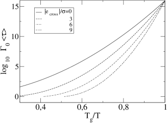
Figure 4: The temperature dependence of $\Gamma_{0}\langle\tau\rangle(\propto D(T))$ for different values of the crossover energy with $\lambda=1$ (the values are given with respect to $e_{0,eff}$).

Note that Eq.34 implies that BMLJ is stronger than BKS-SiO₂ if the cutoff were artificially removed so that the PEL is purely Gaussian. The non-fragile behavior of BMLJ has been already mentioned in Ref.Tarjus et al. (2000).

Of course, since the temperature dependence of $\tau_{\alpha}$ is in general not identical to that of $\langle\tau\rangle$ the results would slightly differ if $m_{kin,K}$ is calculated for $\tau_{\alpha}$ or $\eta$ rather than for the diffusivity.

Empirical relations to correlate the fragility with, e.g., the Poisson ratio have been suggested Novikov and Sokolov (2003) but are questioned in Yannopoulos and Johari (2006). It would be interesting to check whether there exists a physical connection between the observables, suggested in that work, and the value of $e_{cross}$, determining the crossover from liquid-like behavior to solid-like behavior.

IV.2 Relation to the AG approach

Alternatively, one can calculate the value of $\beta_{g}$ under the assumption of the AG relation Eq.1 and a Gaussian PEL (using $\beta_{harm}=0$). Then one has to solve the equation

$$10^{K}=\exp(\beta_{g}B_{AG}/(\alpha-\beta_{g}^{2}\sigma^{2}/2N).$$ (35)

For large $K$ one obtains

$$\beta_{g}=\frac{\sqrt{2\alpha N}}{\sigma}-\frac{B_{AG}\sqrt{N}}{\sigma K\ln(10)}.$$ (36)

Then a straightforward calculation yields for the fragility (again in the limit of large $K$)

$$m_{kin,K}=\frac{\sqrt{2\alpha}K^{2}(\ln 10)^{2}\sigma}{B_{AG}\sqrt{N}}.$$ (37)

Within the AG-approach the fragility depends on the density of states, i.e. $\alpha$, as well as the empirical constant $B_{AG}$. A large number of states implies larger fragility (at least for fixed $B_{AG}$ which, of course, could also depend on $\alpha$ G. Ruocco, F. Sciortino, F. Zamponi, C. De Micheleand T. Scopigno (2004)).

It may be interesting to compare this relation with the fragility Eq.34, obtained for an IGGF. Qualitatively, both relations would show a somewhat similar behavior if systems with large $\alpha$ are related to systems with a low crossover energy $e_{cross}$, i.e. large $k_{entro}$. This is not unreasonable because in the spirit of percolation-like arguments for a larger number of IS the system would be able to find a path with a lower barrier to move between two low-energy IS. However, in a strict way it will not be possible to map Eq.37 on Eq.34 because of the different $K$-dependence. Formally, this problem could be solved if $\alpha$ decreases with increasing $K$, i.e. going to longer time scales and thus lower glass transition temperatures. Qualitatively this statement is equivalent to the requirement that $G(e)$ decays faster than a Gaussian. This has been suggested in Matyushov and Angell (2005). Physically this might, e.g., occur as a consequence of a broadened low-energy cutoff.

IV.3 Thermodynamic fragility

In the spirit of the thermodynamic fragility as discussed in Martinez and Angell (2001); Wang et al. (2006) one can define the thermodynamic fragility index via G. Ruocco, F. Sciortino, F. Zamponi, C. De Micheleand T. Scopigno (2004)

$$m_{thermo,K}=-\beta_{g}\frac{S_{c}^{\prime}(\beta_{g})}{S_{c}(\beta_{g})}.$$ (38)

We obtain, using Eq.9,

$$m_{thermo,K}=\frac{\sigma^{2}(\beta_{g}-\beta_{harm})\beta_{g}}{N\alpha-\sigma^{2}(\beta_{g}-\beta_{harm})^{2}/2}.$$ (39)

Note that the denominator must be positive because otherwise the entropy of the system would be negative. Under this condition, an increase of $\sigma k_{entro}$ (which is the only relevant dimensionless parameter, characterizing IGGF) and thus of $\sigma\beta_{g}$ (via Eq. 33), gives rise to an increase of $m_{thermo}$ and $m_{kin}$, independent of the values of $\beta_{g}$ or $\alpha$. This strong correlation of $m_{kin}$ and $m_{thermo}$ is in agreement with the experimental observation for most systems Martinez and Angell (2001).

Interestingly, increasing the value of $\beta_{harm}$ yields a decrease in $m_{thermo,K}$. However, a different behavior emerges if one includes the vibronic contribution into the entropy, i.e. by using $S_{ex}(T)=S_{c}(T)+S_{harm}(T)$ rather $S_{c}(T)$. A straightforward calculations yields $S_{ex}(T,\beta_{harm})=S_{c}(T,-\beta_{harm})$, thereby neglecting a constant and a term, depending logarithmically on $\beta$ Heuer (2008). Accordingly, when defining $m_{kin,K}$ on the basis of $S_{ex}(T)$ one obtains an increasing thermodynamic fragility for increasing $\beta_{harm}$ in agreement with the qualitative discussion in Martinez and Angell (2001).

If the cutoff starts to influence the system a detailed calculation is no longer possible because the behavior of the configurational entropy at low temperatures depends on the details of $G(e)$ at low energies. Thus, it is not surprising that for SiO₂ the thermodynamic fragility does not follow the general trend Martinez and Angell (2001).

The present discussion complements the work by Sastry (2001) where the kinetic and the thermodynamic fragility have been discussed with reference to the AG-relation. Simulations have also revealed a significant correlation between both fragilities.

IV.4 Relaxation properties

Here we ask for the probability $S_{0}(t)$ that a system in equilibrium has not performed a hopping process until time $t$. It is given by

$$S_{0}(t)=\int de\,p_{eq}(e)\exp(-\Gamma(e)t).$$ (40)

In what follows the trivial factor $\exp(\beta V_{0})$ will be omitted. For sufficiently low temperatures the decay of this function can be related to the structural relaxation Berthier et al. (2005); Rubner and Heuer (2007).

As shown in Castaing and Souletie (1991); Heuer (2008) one can approximate for intermediate times ($S_{0}(t)\approx 1/e)$

$$S_{0}(t)\approx\exp(-(t/\tau_{KWW})^{\beta_{KWW}})$$ (41)

with

$$\beta_{KWW}=1/\sqrt{1+\mu^{2}}$$ (42)

and $\tau_{KWW}=1/\Gamma^{\star}$ where

$$\Gamma^{\star}=\Gamma(\langle e(T)\rangle)=\exp(-\mu^{2}).$$ (43)

This may justify the use of the stretched exponential as a fitting function at least for intermediate times. This result is insensitive to the specific form of $\Gamma(e)$ since $\Gamma(e)$ only enters via $\Gamma^{\star}$. Note that for the IGGF the non-exponentiality tends to increase when going to lower temperatures. Furthermore one can show that in very long-time decay is algebraic Castaing and Souletie (1991); Heuer (2008)

$$S_{0}(t)\propto t^{-u/2\mu^{2}}.$$ (44)

One can define the $\alpha$-relaxation time $\tau_{\alpha}$ via

$$\tau_{\alpha}=\int\,dt\,S_{0}(t)$$ (45)

which corresponds to the typical time until a particle jumps for the first time Berthier et al. (2005); Rubner and Heuer (2007). From Eq. 40 one immediately obtains (also using Eq.30)

$$\tau_{\alpha}=\langle\Gamma^{-1}\rangle_{p}=(1/\Gamma_{0})\exp(3\mu^{2}/2).$$ (46)

This has to be compared with the average hopping time $\langle\tau\rangle$ (Eq.27). One obtains

$$\tau_{\alpha}/\langle\tau\rangle=\exp(\mu^{2}).$$ (47)

Since the left side is proportional to $D\tau_{\alpha}$ Eq.47 expresses the invalidation of the Stokes-Einstein relation for IGGF. Using the definition of the exponent $a$ via $D(T)\tau_{\alpha}(T)\propto\tau_{\alpha}^{a}$ , i.e. $\langle\Gamma\rangle\langle\Gamma^{-1}\rangle\propto\langle\Gamma^{-1}\rangle^{\alpha}$ one obtains $a=2/3$. Experimental values are smaller (e.g. 0.25 for orthoterphenyl Fujara et al. (1992) and 0.23 for TNB Swallen et al. (2003)). Thus, the decoupling seems to be too strong. Qualitatively the strong increase of $\tau_{\alpha}$ with decreasing temperature is due to the very long-time tail of $S_{0}(t)$.

V Discussion and Summary

The IGGF has been introduced, based on the numerical results for BMLJ and BKS-SiO₂ (except for the low-energy cutoff for BKS-SiO₂) at small system sizes. The general concepts are also compatible with several models proposed to rationalize the dynamics of supercooled liquids. Thus, one naturally finds how properties such as the non-exponentiality are generated.

More specifically, the key conclusions are as follows: 1.) If the cutoff-energy does not interfere the temperature-dependence of the dynamics is fully captured by the value of $\mu$ (except for a trivial $\exp(-\beta V_{0})$-term). This means in particular that at $T_{g}$ an IGGF has a fixed value of $\mu$, independent of $\sigma k_{entro}$ and thus independent of its fragility. This implies via Eq.42 that the stretching parameter $\beta_{KWW}$ does not depend on the fragility if determined exactly at $T_{g}$. This may rationalize the weak correlation between $\beta_{KWW}$ and $m_{kin}$ for the molecular glass-forming systems, as mentioned above. Of course, residual fluctuations are expected when the smaller-order effects of $\lambda$, $\kappa$ and $V_{0}$ are taken into account. 2.) The fragility of a system is to a large extent dominated by the crossover energy $e_{cross}$ relative to the width of the energy distribution, i.e. $\sigma$. Systems are more fragile if the crossover from solid-like activated dynamics to liquid-like non-activated dynamics occurs at low energies, relative to the width of $G(e)$. Of course, as soon as the low-energy cutoff of the PEL comes into play (such as for BKS-SiO₂) the system automatically behaves Arrhenius-like and thus is classified as strong. This also shows that the fragility is only partly able to classify a glass-forming system because already the present discussion shows that there at least two very different parameters, $e_{cut}$ and $e_{cross}$, which strongly influence the fragility. 3.)Although the BMLJ data can be fit to the AG-relation, from a conceptual point of view the IGGF is not compatible with the AG-relaxation. This can be seen from the different dependence of the fragility on $K$. On a qualitative level this discrepancy could be reduced if the distribution of states decays stronger than a Gaussian at the low-energy end. 4.) The thermodynamic fragility indeed is correlated with the kinetic fragility, albeit in a non-trivial way. Again, the systems with a cutoff-behavior (most notably BKS-SiO₂) have to be discussed separately. 5.) Finally, the IGGF displays non-exponential relaxation with a non-exponentiality which increases with decreasing temperature and, in agreement with the experiment, shows a violation of the Stokes-Einstein relation.

Conceptually, the presence of individual relaxation processes naturally is attributed to small systems, reflecting the typical length scales of cooperative dynamics during single MB transitions. Thus, any strict comparison with simulations in the framework of the PEL approach is conveniently performed with small systems. As shown in previous work the diffusion constant as well as the thermodynamic properties of the BMLJ ($N=65)$-system only have very minor finite-size effects when comparing with the results obtained for much larger systems Buechner and Heuer (1999); Doliwa and Heuer (2003e); Stariolo and Fabricius (2006). However, the structural relaxation time as the well as the non-exponentiality has somewhat larger finite-size effects Stariolo and Fabricius (2006). This effect can be understood if one assumes a specific type of coupling between adjacent subsystems of a larger system. When some subsystem relaxes it may change the mobility of the adjacent subsystems Heuer (2008). A similar idea can be already found in Bouchaud et al. (1995); Monthus and Bouchaud (1996) and has been also implemented in the context of the rate memory to explain the results of multidimensional NMR experiments Heuer et al. (1995); Sillescu (1996); Heuer (1997); Diezemann (1997). In this way the very immobile regions typically become mobile at some stage and can relax subsequently. In some sense this idea is also related to the philosophy of the facilitated spin models where the local mobility is also influenced by the state of the neighbor spins Fredrickson and Andersen (1984); Garrahan and Chandler (2002); Berthier and Garrahan (2003). The coupling between adjacent subsystems can be formulated such that the diffusion constant and the thermodynamics does not change whereas the structural relaxation time, all moments $\langle\tau^{n}\rangle$ for $n\geq 2$ and the degree of non-exponentiality decrease upon this coupling Heuer (2008). This might also explain why the second moment for the BMLJ system is by a factor of 2 smaller than expected (see above). In particular the exponent $a$, characterizing the violation of the Stokes-Einstein equation approaches experimentally relevant values Heuer (2008). However, one of the key results, namely the utmost relevance of a single dimensionless parameter $\mu$ would still be valid. In any event, the path back from small systems to macroscopic systems is one of the challenges for future work. Using the IGGS as the elementary system for such models is definitely a reasonable starting point.

We gratefully acknowledge important input from C. Rehwald and O. Rubner as well as very helpful correspondence with L. Berthier about this topic.

References

- P. G. Debenedetti and F. H. Stillinger (2001) P. G. Debenedetti and F. H. Stillinger, Nature 410, 259 (2001).
- Binder and Kob (2005) K. Binder and W. Kob, Glassy materials and disordered solids (World Scientific, 2005).
- Dyre (2006) J. C. Dyre, Rev. Mod. Phys. 78, 953 (2006).
- Lubchenko and Wolyness (2006) V. Lubchenko and P. G. Wolyness, Ann. Rev. Phys. Chem. 58, 235 (2006).
- Hurley and Harrowell (1995) M. Hurley and P. Harrowell, Phys. Rev. E 52, 1694 (1995).
- Kob et al. (1997) W. Kob, C. Donati, S. J. Plimpton, P. H. Poole, and S. C. Glotzer, Phys. Rev. Lett. 79, 2827 (1997).
- Donati et al. (1998) C. Donati, J. F. Douglas, W. Kob, S. J. Plimpton, P. H. Poole, and S. C. Glotzer, Phys. Rev. Lett. 80, 2338 (1998).
- Donati et al. (1999a) C. Donati, S. C. Glotzer, P. H. Poole, W. Kob, and S. J. Plimpton, Phys. Rev. E 60, 3107 (1999a).
- Donati et al. (1999b) C. Donati, S. C. Glotzer, and P. H. Poole, Phys. Rev. Lett. 82, 5064 (1999b).
- Heuer and Okun (1997) A. Heuer and K. Okun, J. Chem. Phys. 106, 6176 (1997).
- Qian et al. (1999) J. Qian, R. Hentschke, and A. Heuer, J. Chem. Phys. 110, 4514 (1999).
- Wales (2003) D. J. Wales, Energy landscapes (Cambridge University Press, 2003).
- Sciortino (2005) F. Sciortino, J. Stat. Mech. P05015 (2005).
- Stillinger and Weber (1982) F. H. Stillinger and T. A. Weber, Phys. Rev. A 25, 978 (1982).
- Stillinger and Weber (1984) F. H. Stillinger and T. A. Weber, Science 225, 983 (1984).
- Schrøder et al. (2000) T. B. Schrøder, S. Sastry, J. C. Dyre, and S. C. Glotzer, J. Chem. Phys. 112, 9834 (2000).
- F. H. Stillinger (1995) F. H. Stillinger, Science 267, 1935 (1995).
- Middleton and Wales (2001) T. F. Middleton and D. J. Wales, Phys. Rev. B 64, 024205 (2001).
- Doliwa and Heuer (2003a) B. Doliwa and A. Heuer, Phys. Rev. E 67, 030501 (2003a).
- Doliwa and Heuer (2003b) B. Doliwa and A. Heuer, Phys. Rev. E 67, 031506 (2003b).
- Denny et al. (2003) R. A. Denny, D. R. Reichman, and J. P. Bouchaud, Phys. Rev. Lett. 90, 025503 (2003).
- Adam and Gibbs (1965) G. Adam and J. H. Gibbs, J. Chem. Phys. 43, 139 (1965).
- Martinez and Angell (2001) L. Martinez and C. Angell, Nature 410, 663 (2001).
- Wang et al. (2006) L.-M. Wang, C. A. Angell, and R. Richert, J. Chem. Phys. 125, 074505 (2006).
- G. Ruocco, F. Sciortino, F. Zamponi, C. De Micheleand T. Scopigno (2004) G. Ruocco, F. Sciortino, F. Zamponi, C. De Micheleand T. Scopigno, J. Chem. Phys. 120, 10666 (2004).
- Angell (2000) C. A. Angell, J. Phys.-Condes. Matter 12, 6463 (2000).
- Fujara et al. (1992) F. Fujara, B. Geil, H. Sillescu, and G. Fleischer, Z. Phys. B 88, 195 (1992).
- Bohmer et al. (1993) R. Bohmer, K. L. Ngai, C. A. Angell, and D. J. Plazek, J. Chem. Phys. 99, 4201 (1993).
- Heuer (2008) A. Heuer, (submitted) (2008).
- Sciortino et al. (1999a) F. Sciortino, W. Kob, and P. Tartaglia, Phys. Rev. Lett. 83, 3214 (1999a).
- Buechner and Heuer (1999) S. Buechner and A. Heuer, Phys. Rev. E 60, 6507 (1999).
- Starr et al. (2001) F. W. Starr, S. Sastry, E. La Nave, A. Scala, H. E. Stanley, and F. Sciortino, Phys. Rev. E 63, 041201 (2001).
- Nave et al. (2000) E. L. Nave, S. Mossa, F. S. F, and P. Tartaglia, J. Chem. Phys. 120, 6128 (2000).
- Saksaengwijit et al. (2004) A. Saksaengwijit, J. Reinisch, and A. Heuer, Phys. Rev. Lett. 93, 235701 (2004).
- Doliwa and Heuer (2003c) B. Doliwa and A. Heuer, Phys. Rev. Lett. 91, 235501 (2003c).
- Monthus and Bouchaud (1996) C. Monthus and J. P. Bouchaud, J. Phys. A-Math. Gen. 29, 3847 (1996).
- Sciortino et al. (1999b) F. Sciortino, W. Kob, and P. Tartaglia, Phys. Rev. Lett. 83, 3214 (1999b).
- Buechner and Heuer (2000) S. Buechner and A. Heuer, Phys. Rev. Lett. 84, 2168 (2000).
- Saksaengwijit and Heuer (2006a) A. Saksaengwijit and A. Heuer, Phys. Rev. E 74, 051502 (2006a).
- Saika-Voivod et al. (2004) I. Saika-Voivod, F. Sciortino, and P. H. Poole, Phys. Rev. E. 69, 041503 (2004).
- Sastry (2001) S. Sastry, Nature 409, 164 (2001).
- Mossa et al. (2002) S. Mossa, E. La Nave, H. E. Stanley, C. Donati, F. Sciortino, and P. Tartaglia, Phys. Rev. E 65, 041205 (2002).
- Giovambattista et al. (2003) N. Giovambattista, H. E. Stanley, and F. Sciortino, Phys. Rev. Lett. 91, 115504 (2003).
- Sciortino et al. (2003) F. Sciortino, E. L. Nave, and P. Tartaglia, Phys Rev. Lett. 91, 155701 (2003).
- Brawer (1984) S. Brawer, J. Chem. Phys. 81, 954 (1984).
- Dyre (1987) J. C. Dyre, Phys. Rev. Lett. 58, 792 (1987).
- Arkhipov and Baessler (1994) V. Arkhipov and H. Baessler, J. Phys. Chem. 98, 662 (1994).
- Diezemann (1997) G. Diezemann, J. Chem. Phys. 107, 10112 (1997).
- Diezemann et al. (1998) G. Diezemann, H. Sillescu, G. Hinze, and R. Bohmer, Phys. Rev. E 57, 4398 (1998).
- Dyre (1995) J. C. Dyre, Phys. Rev. B 51, 12276 (1995).
- Brawer (1985) S. Brawer, Relaxation in Viscous Liquids and Glasses (The American Ceramic Society, Inc., 1985).
- Saksaengwijit and Heuer (2006b) A. Saksaengwijit and A. Heuer, Phys. Rev. E 73, 061503 (2006b).
- de Souza and Wales (2006) V. de Souza and D. Wales, Phys. Rev. Lett. 96, 057802 (2006).
- La Nave et al. (2002) E. La Nave, H. E. Stanley, and F. Sciortino, Phys. Rev. Lett 88, 035501 (2002).
- Doliwa and Heuer (2003d) B. Doliwa and A. Heuer, Phys. Rev. E. 67, 031506 (2003d).
- Berthier et al. (2005) L. Berthier, D. Chandler, and J. Garrahan, Europhys. Lett. 69, 320 (2005).
- Rubner and Heuer (2007) O. Rubner and A. Heuer, (in preparation) (2007).
- Heuer et al. (2005) A. Heuer, B. Doliwa, and A. Saksaengwijit, Phys. Rev. E 72, 021503 (2005).
- Schmidt-Rohr and Spiess (1991) K. Schmidt-Rohr and H. Spiess, Phys. Rev. Lett. 66, 3020 (1991).
- Richert (1993) R. Richert, Chem. Phys. Lett. 216, 223 (1993).
- Bohmer et al. (1998) R. Bohmer, R. V. Chamberlin, G. Diezemann, B. Geil, A. Heuer, G. Hinze, S. C. Kuebler, R. Richert, B. Schiener, H. Sillescu, et al., J. Non-Cryst. Solids 235, 1 (1998).
- Tarjus et al. (2000) G. Tarjus, D. Kivelson, and P. Viot, J. Phys.: Cond. Mat. 12, 6497 (2000).
- Novikov and Sokolov (2003) V. H. Novikov and A. P. Sokolov, Nature 431, 961 (2003).
- Yannopoulos and Johari (2006) S. N. Yannopoulos and G. P. Johari, Nature 442, E7 (2006).
- Matyushov and Angell (2005) D. Matyushov and C. Angell, J. Chem. Phys. 123, 034506 (2005).
- Castaing and Souletie (1991) B. Castaing and J. Souletie, J. Phys. I 1, 403 (1991).
- Swallen et al. (2003) S. Swallen, P. Bonvallet, R. McMahon, and M. Ediger, Phys. Rev. Lett. 90, 015901 (2003).
- Doliwa and Heuer (2003e) B. Doliwa and A. Heuer, J. Phys. C: Cond. Mat. 15, S849 (2003e).
- Stariolo and Fabricius (2006) D. A. Stariolo and G. Fabricius, J. Chem. Phys. 125, 064505 (2006).
- Bouchaud et al. (1995) J. P. Bouchaud, A. Comtet, and C. Monthus, J. Phys. I 5, 1521 (1995).
- Heuer et al. (1995) A. Heuer, M. Wilhelm, H. Zimmermann, and H. Spiess, Phys. Rev. Lett. 75, 2851 (1995).
- Sillescu (1996) H. Sillescu, J. Chem. Phys. 104, 4877 (1996).
- Heuer (1997) A. Heuer, Phys. Rev. E 56, 730 (1997).
- Fredrickson and Andersen (1984) G. Fredrickson and H. Andersen, Phys. Rev. Lett. 53, 1244 (1984).
- Garrahan and Chandler (2002) J. P. Garrahan and D. Chandler, Phys. Rev. Lett. 89, 035704 (2002).
- Berthier and Garrahan (2003) L. Berthier and J. P. Garrahan, Phys. Rev. E. 68, 041201 (2003).