Relativistic stars with purely toroidal magnetic fields

Abstract

We investigate the effects of the purely toroidal magnetic field on the equilibrium structures of the relativistic stars. The master equations for obtaining equilibrium solutions of relativistic rotating stars containing purely toroidal magnetic fields are derived for the first time. To solve these master equations numerically, we extend the Cook-Shapiro-Teukolsky scheme for calculating relativistic rotating stars containing no magnetic field to incorporate the effects of the purely toroidal magnetic fields. By using the numerical scheme, we then calculate a large number of the equilibrium configurations for a particular distribution of the magnetic field in order to explore the equilibrium properties. We also construct the equilibrium sequences of the constant baryon mass and/or the constant magnetic flux, which model the evolution of an isolated neutron star as it loses angular momentum via the gravitational waves. Important properties of the equilibrium configurations of the magnetized stars obtained in this study are summarized as follows ; (1) For the non-rotating stars, the matter distribution of the stars is prolately distorted due to the toroidal magnetic fields. (2) For the rapidly rotating stars, the shape of the stellar surface becomes oblate because of the centrifugal force. But, the matter distribution deep inside the star is sufficiently prolate for the mean matter distribution of the star to be prolate. (3) The stronger toroidal magnetic fields lead to the mass-shedding of the stars at the lower angular velocity. (4) For some equilibrium sequences of the constant baryon mass and magnetic flux, the stars can spin up as they lose angular momentum.

I Introduction

There is growing evidence for the existence of so-called magnetars, supermagnetized neutron stars with the magnetic fields of $\sim 10^{14}-10^{15}$ G (e.g., Lattimer:2006 ; wod ). Although such stars are estimated to be only a subclass ($\sim 10\%$) of the canonical neutron stars with $\sim 10^{12}-10^{13}$ G kouve , much attention has been paid to the objects because they pose many astrophysically exciting but unresolved problems. Giant flaring activities in the soft gamma repeaters observed for the last two decades have given us good opportunities to study the coupling of the interior to the magnetospheric structures of magnetars Thompson:1995gw ; Thompson:1996pe , but the relationship between the crustal fraction and the subsequent star quarks has not yet been clarified (see references in anna ; Geppert:2006cp ). The origin of the large magnetic field is also a big problem, whether generated at post-collapse in the rapidly rotating neutron star Thompson:1993hn or descended from the main sequence stars Ferrario:2007bt . Assuming large magnetic fields before core-collapse, researches have recently performed extensive magnetohydrodynamic (MHD) stellar collapse simulations Yamada:2004 ; Kotake:2004 ; Moissenko:2006 ; Obergaulinger:2006 ; Shibata:2006hr ; Livne:2007 in order to understand the formation mechanism of magnetars, with different levels of sophistication in the treatment of equations of state (EOSs), the neutrino transport, and general relativity (see Kotake:2006 for a review). Here it is worth mentioning that the gravitational waves from magnetars could be a useful source of information about magnetar interiors  Bonazzola:1995rb ; Cutler:2002nw . From a microscopic point of view, the effects of magnetic field larger than the so-called QED limit of $\sim 4.4\times 10^{13}~{}\rm{G}$, on the EOSs (e.g., Lattimer:2006 ) and the radiation processes have been also extensively investigated (see Harding:2006 for a review). For the understanding of the formation and evolution of the magnetars, it is indispensable to unify these macroscopic and microscopic studies, albeit not an easy job.

When one tries to study the above interesting issues, the construction of an equilibrium configuration of magnetars may be one of the most fundamental problems. In spite of the many magnetized star investigations that have so far been carried out, with different levels of sophistication in the treatment of the magnetic field structure, equations of state (EOSs), and the general relativity Bocquet:1995 ; Ioka:2003 ; Ioka:2004 ; Kiuchi:2007pa ; Konno:1999zv ; Tomimura:2005 ; Yoshida:2006a ; Yoshida:2006b , there still remains room for more sophistication in the previous studies in which stellar structures are obtained within the framework of Newtonian dynamics. Since we are interested in magnetar structures, the general relativistic treatment due to the strong gravity of magnetars is required in constructions of a magnetar model. However, a fully general relativistic means constructing a stellar model with arbitrarily magnetic structure are still not available. In most studies on the structures of relativistic magnetized stars, weak magnetic fields and/or purely poloidal magnetic fields have been assumed. Bocquet et al. Bocquet:1995 and Cardall et al. Cardall:2001 have treated relativistic stellar models containing purely poloidal magnetic fields. Konno et al. Konno:1999zv have analyzed similar models using a perturbative approach. Ioka and Sasaki have investigated structures of mixed poloidal-toroidal magnetic fields around a spherical star by using a perturbative technique Ioka:2004 .

As shown in core-collapse supernova MHD simulations (see, e.g., Kotake:2006 ), the toroidal magnetic fields can be easily amplified because of the winding up of the initial seed poloidal fields as long as the core is rotating differentially. After core bounce, as a result, the toroidal fields dominate over the poloidal ones in some proto-neutron star models even if there is no toroidal field initially. This winding up amplification of the toroidal magnetic fields therefore indicates that some neutron stars could have toroidal fields much higher than poloidal ones. As mentioned before, however, no effect of a strong toroidal magnetic field has been taken into account in relativistic magnetized stellar models. In order to elucidate the effects of strong toroidal magnetic fields on neutron star structures, in this paper, we concentrate on magnetic effects due to purely toroidal fields on structures of relativistic stars as a first step. Within the framework of the Newtonian dynamics, Miketinac has obtained highly magnetized stars containing purely toroidal magnetic fields Miketinac:1973 . In this study, we extend Miketinac’s models so as to include the effects of general relativity and rotation.

First of all, we derive master equations for obtaining relativistic rotating stellar models having purely toroidal magnetic fields. The master equations obtained are converted into integral expressions and solved numerically with a self-consistent field scheme similar to the Komatsu-Eriguchi-Hachisu scheme for equilibrium structures of relativistic rotating stars Komatsu:1989 . Using the numerical scheme written in the present study, we construct a large number of equilibrium stars for a wide range of parameters. As shown by Trehan & Uberoi trehan1972 , the toroidal magnetic field tends to distort a stellar shape prolately. This is because the toroidal magnetic field lines behave like a rubber belt, pulling in the matter around the magnetic axis. Such a prolate-shaped neutron star may be an optimal source of gravitational waves if the star rotates Cutler:2002nw . In this gravitational wave emission mechanism, one important parameter is degree of prolateness, which determines the amount of gravitational radiation. Thus, we pay attention to the deformation of the star. We also construct sequences of the equilibrium stars along which the total baryon rest mass and/or the magnetic flux with respect to the meridional cross-section keep constant. These equilibrium sequences are available for exploring evolutionary sequences because the total baryon rest mass and the magnetic flux are well conserved in quasi-steady evolution of isolated neutron stars.

This paper is organized as follows. The master equations for obtaining equilibrium configurations of rotating stars with purely toroidal magnetic fields are derived in Sec. II. The numerical scheme for computing the stellar models is briefly described in Sec. III. Sec. IV is devoted to showing numerical results. Summary and discussion follow in Sec. V. In this paper, we use geometrical units with $G=c=1$.

II Master equations

II.1 Matter equations

The rotating relativistic stars containing purely toroidal magnetic fields are considered in this paper. Assumptions to obtain the equilibrium models are summarized as follows ; (1) Equilibrium models are stationary and axisymmetric, i.e. the spacetime has the time Killing vector, $t^{\mu}$, and the rotational Killing vector, $\varphi^{\mu}$, and Lie derivatives of the physical quantities of the equilibrium models with respect to these Killing vectors vanish. (2) The matter source is approximated by a perfect fluid with infinite conductivity. (3) There is no meridional flow of the matter. (4) The equation of state for the matter is barotropic. By virtue of assumption (3), the matter four-velocity is reduced to

$$u^{\mu}=u^{0}(t^{\mu}+\Omega\varphi^{\mu}),$$ (1)

where $\Omega$ is the angular velocity of the matter. We further assume that the magnetic field of the star has toroidal parts only, so that the Faraday tensor, $F_{\mu\nu}$, obeys the conditions, given by

$$F_{\mu\nu}\,t^{\nu}=0\,,\quad F_{\mu\nu}\,\varphi^{\nu}=0\,.$$ (2)

Note that since Eq. (2) includes five independent conditions, we see that the Faraday tensor has one independent component only. Thanks to the conditions assumed above, one of the Maxwell equations and the perfect-conductivity condition,

$$F_{[\mu\nu,\alpha]}=0,$$ (3)

$$F_{\mu\nu}u^{\nu}=0,$$ (4)

are automatically satisfied, and we need not consider them any further. The stress-energy tensor of the perfectly conductive fluid is given by

$$T^{\mu\nu}=(\rho_{0}+\rho_{0}e+P)u^{\mu}u^{\nu}+Pg^{\mu\nu}+\frac{1}{4\pi}\left[B^{\alpha}B_{\alpha}\left(u^{\mu}u^{\nu}+\frac{1}{2}g^{\mu\nu}\right)-B^{\mu}B^{\nu}\right],$$ (5)

where $\rho_{0}$ is the rest energy density, $e$ the specific internal energy, $P$ the pressure, and $g^{\mu\nu}$ the inverse of the metric $g_{\mu\nu}$. Here, we have defined the magnetic field measured by the observer with the fluid four-velocity $u^{\mu}$ as

$$B^{\mu}=-\frac{1}{2}\epsilon^{\mu\nu\alpha\beta}u_{\nu}F_{\alpha\beta},$$ (6)

where $\epsilon^{\mu\nu\alpha\beta}$ stands for the contravariant Levi-Civita tensor with $\epsilon^{0123}=-1/\sqrt{-g}$. Here $g$ denotes the determinant of the metric. By using Eqs. (1)–(2), (4)–(5), and (6), we can prove that the circularity condition, i.e., $t_{\alpha}T^{\alpha[\beta}t^{\gamma}\varphi^{\delta]}=\varphi_{\alpha}T^{\alpha[\beta}t^{\gamma}\varphi^{\delta]}=0$, is satisfied in the present situation Wald:1984 . Note that a similar argument about the circularity has been given by Oron Oron: 2002 . Therefore, there exists a family of two-surfaces everywhere orthogonal to the plane defined by the two Killing vectors $t^{\mu}$ and $\varphi^{\mu}$ Carter:1969 , and the metric can be written, following Komatsu:1989 ; Cook:1992 , in the form

$$ds^{2}=-{\rm e}^{\gamma+\rho}dt^{2}+{\rm e}^{2\alpha}(dr^{2}+r^{2}d\theta^{2})+{\rm e}^{\gamma-\rho}r^{2}\sin^{2}\theta(d\varphi-\omega dt)^{2},$$ (7)

where the metric potentials, $\gamma$, $\rho$, $\alpha$, and $\omega$, are functions of $r$ and $\theta$ only. We see that the non-zero component of $F_{\mu\nu}$ in this coordinate is $F_{12}$. It is convenient to define the determinants of two two-dimensional subspaces for later discussion,

$$g_{A} \equiv g_{11}g_{22}-(g_{12})^{2}={\rm e}^{4\alpha}\,r^{2},~{}~{}$$

$$g_{B} \equiv -g_{00}g_{33}+(g_{03})^{2}={\rm e}^{2\gamma}\,r^{2}\sin^{2}\theta,$$ (8)

where the determinant of the metric (7) is related to the two determinants as $g=-g_{A}g_{B}$. We then find a convenient relation,

$$F_{12}=g_{A}F^{12}.$$ (9)

Because of this relation, the four-current $J^{\mu}$ can, in terms of $F_{12}$, be written in the form,

$$J^{\alpha} = \frac{1}{4\pi}\frac{1}{\sqrt{-g}}\partial_{\beta}(\sqrt{-g}F^{\alpha\beta})$$ (10)

$$= \frac{1}{4\pi}\frac{1}{\sqrt{g_{A}g_{B}}}\left[-\partial_{1}\left(\sqrt{\frac{g_{B}}{g_{A}}}F_{12}\right)\delta^{\alpha}_{2}+\partial_{2}\left(\sqrt{\frac{g_{B}}{g_{A}}}F_{12}\right)\delta^{\alpha}_{1}\right].$$

The relativistic Euler equation,

$$u^{\nu}\nabla_{\nu}u^{\mu}+\frac{1}{\rho_{0}h}\nabla_{\mu}P-\frac{1}{\rho_{0}h}F_{\mu\nu}J^{\nu}=0,$$ (11)

is reduced to

$$-\partial_{A}\ln u^{0}+\frac{1}{\rho_{0}h}\partial_{A}P+\frac{1}{4\pi\rho_{0}hg_{B}}\sqrt{\frac{g_{B}}{g_{A}}}F_{12}\partial_{A}\left(\sqrt{\frac{g_{B}}{g_{A}}}F_{12}\right)=0,$$ (12)

where $h=1+e+P/\rho_{0}$ is the specific enthalpy and we have assumed the uniform rotation, i.e., $\Omega={\rm constant}$. Note that although the extension to the case of the differential rotation is straightforward, we take the uniform rotation law for the sake of simplicity. Integrability of Eq. (12) requires

$$\sqrt{\frac{g_{B}}{g_{A}}}F_{12}=K(u);~{}~{}~{}u\equiv\rho_{0}hg_{B},$$ (13)

where $K$ is an arbitrary function of $\rho_{0}hg_{B}$. Integrating Eq. (12), we arrive at the equation of hydrostatic equilibrium,

$$\ln h-\ln u^{0}+\frac{1}{4\pi}\int\frac{K(u)}{u}\frac{dK}{du}du=C,$$ (14)

where $C$ is an integral constant. The nontrivial components of the magnetic field are explicitly given by

$$B_{0}=-\Omega u^{0}K(u),$$ (15)

$$B_{3}=u^{0}K(u),$$ (16)

in which we confirm that our definition of the toroidal magnetic field (2) reasonably agrees with the Newtonian definition of the toroidal field.

With the metric (7), the four-velocity (1), the proper velocity of the matter with respect to a zero angular momentum observer (ZAMO), $v$, the components of the magnetic field (15)-(16), and the hydrostatic equilibrium equation (14) can be, respectively, written as

$$u^{\mu}=\frac{{\rm e}^{-(\rho+\gamma)/2}}{\sqrt{1-v^{2}}}(t^{\mu}+\Omega\varphi^{\mu}),$$ (17)

$$v=(\Omega-\omega)r\sin\theta{\rm e}^{-\rho}.$$ (18)

$$B_{0}=-\frac{{\rm e}^{-(\rho+\gamma)/2}}{{\sqrt{1-v^{2}}}}\Omega K(u),$$ (19)

$$B_{3}=\frac{{\rm e}^{-(\rho+\gamma)/2}}{{\sqrt{1-v^{2}}}}K(u),$$ (20)

$$\ln h+\frac{\gamma+\rho}{2}+\frac{1}{2}\ln(1-v^{2})+\frac{1}{4\pi}\int\frac{K(u)}{u}\frac{dK}{du}du=C.$$ (21)

II.2 Einstein equations

Following Komatsu:1989 ; Cook:1992 , we may write the general relativistic field equations determining $\rho$, $\gamma$ , and $\omega$ as

$$\nabla^{2}[\rho{\rm e}^{\gamma/2}]=S_{\rho}(r,\mu),$$ (22)

$$\left(\nabla^{2}+\frac{1}{r}\partial_{r}-\frac{\mu}{r^{2}}\partial_{\mu}\right)[\gamma{\rm e}^{\gamma/2}]=S_{\gamma}(r,\mu),$$ (23)

$$\left(\nabla^{2}+\frac{2}{r}\partial_{r}-\frac{2\mu}{r^{2}}\partial_{\mu}\right)[\omega{\rm e}^{(\gamma-2\rho)/2}]=S_{\omega}(r,\mu),$$ (24)

where $\nabla^{2}$ is the Laplacian of flat 3-space, and $\mu=\cos\theta$. Here, $S_{\rho}$, $S_{\gamma}$, and $S_{\omega}$ are given by

$$S_{\rho}(r,\mu)={\rm e}^{\gamma/2}\Big{\{}8\pi{\rm e}^{2\alpha}(\rho_{0}+\rho_{0}e+P)\frac{1+v^{2}}{1-v^{2}}+r^{2}(1-\mu^{2}){\rm e}^{-2\rho}\left(\omega_{,r}^{2}+\frac{1-\mu^{2}}{r^{2}}\omega_{,\mu}^{2}\right)$$

$$+\frac{1}{r}\gamma_{,r}-\frac{\mu}{r^{2}}\gamma_{,\mu}+\frac{\rho}{2}\left[16\pi{\rm e}^{2\alpha}\left(P+\frac{|B|^{2}}{8\pi}\right)-\gamma_{,r}\left(\frac{1}{2}\gamma_{,r}+\frac{1}{r}\right)-\frac{1}{r^{2}}\gamma_{,\mu}\left(\frac{1-\mu^{2}}{2}\gamma_{,\mu}-\mu\right)\right]\Big{\}},$$ (25)

$$S_{\gamma}(r,\mu)={\rm e}^{\gamma/2}\left\{16\pi{\rm e}^{2\alpha}\left(P+\frac{|B|^{2}}{8\pi}\right)+\frac{\gamma}{2}\left[16\pi{\rm e}^{2\alpha}\left(P+\frac{|B|^{2}}{8\pi}\right)-\frac{1}{2}\gamma_{,r}^{2}-\frac{1-\mu^{2}}{2r^{2}}\gamma_{,\mu}^{2}\right]\right\},$$ (26)

$$S_{\omega}(r,\mu)={\rm e}^{(\gamma-2\rho)/2}\Big{\{}-16\pi{\rm e}^{2\alpha}\frac{(\Omega-\omega)(\rho_{0}+\rho_{0}e+P)}{1-v^{2}}$$

$$+\omega\Big{[}-8\pi{\rm e}^{2\alpha}\left(\frac{(\rho_{0}+\rho_{0}e+P)(1+v^{2})}{1-v^{2}}-P-\frac{|B|^{2}}{8\pi}\right)-\frac{1}{r}\left(2\rho_{,r}+\frac{1}{2}\gamma_{,r}\right)+\frac{\mu}{r^{2}}\left(2\rho_{,\mu}+\frac{1}{2}\gamma_{,\mu}\right)$$

$$+\frac{1}{4}(4\rho_{,r}^{2}-\gamma_{,r}^{2})+\frac{1-\mu^{2}}{4r^{2}}(4\rho_{,\mu}^{2}-\gamma_{,\mu}^{2})-r^{2}(1-\mu^{2}){\rm e}^{-2\rho}\left(\omega_{,r}^{2}+\frac{1-\mu^{2}}{r^{2}}\omega_{,\mu}^{2}\right)\Big{]}\Big{\}},$$ (27)

where $|B|$ denotes the magnitude of the magnetic field, given by

$$|B|=\frac{|K|{\rm e}^{-\gamma}}{r\sin\theta}.$$ (28)

Since $S_{\rho}$, $S_{\gamma}$, and $S_{\omega}$ do not include the second-order derivative of the metric potentials, the three equations (22)–(24) are all elliptic-type partial differential equations. We can solve these equations iteratively with appropriate boundary conditions by using a self-consistent field method Komatsu:1989 .

The fourth field equation determining $\alpha$ is given by

$$\alpha_{,\mu}=-\frac{1}{2}(\rho_{,\mu}+\gamma_{,\mu})-\{(1-\mu^{2})(1+r\gamma_{,r})^{2}+[\mu-(1-\mu^{2})\gamma_{,\mu}]^{2}\}^{-1}\Big{[}$$

$$\frac{1}{2}[r^{2}(\gamma_{,rr}+\gamma_{,r}^{2})-(1-\mu^{2})(\gamma_{,\mu\mu}+\gamma_{,\mu}^{2})][-\mu+(1-\mu^{2})\gamma_{,\mu}]+r\gamma_{,r}\left[\frac{1}{2}\mu+\mu r\gamma_{,r}+\frac{1}{2}(1-\mu^{2})\gamma_{,\mu}\right]$$

$$+\frac{3}{2}\gamma_{,\mu}[-\mu^{2}+\mu(1-\mu^{2})\gamma_{,\mu}]-r(1-\mu^{2})(\gamma_{,r\mu}+\gamma_{,r}\gamma_{,\mu})(1+r\gamma_{,r})-\frac{1}{4}\mu r^{2}(\rho_{,r}+\gamma_{,r})^{2}$$

$$-\frac{r}{2}(1-\mu^{2})(\rho_{,r}+\gamma_{,r})(\rho_{,\mu}+\gamma_{,\mu})+\frac{1}{4}\mu(1-\mu^{2})(\rho_{,\mu}+\gamma_{,\mu})^{2}-\frac{r^{2}}{2}(1-\mu^{2})\gamma_{,r}(\rho_{,r}+\gamma_{,r})(\rho_{,\mu}+\gamma_{,\mu})$$

$$+\frac{1}{4}(1-\mu^{2})\gamma_{,\mu}[r^{2}(\rho_{,r}+\gamma_{,r})^{2}-(1-\mu^{2})(\rho_{,\mu}+\gamma_{,\mu})^{2}]+(1-\mu^{2})e^{-2\rho}\Big{\{}\frac{1}{4}r^{4}\mu\omega_{,r}^{2}+\frac{1}{2}r^{3}(1-\mu^{2})\omega_{,r}\omega_{,\mu}$$

$$-\frac{1}{4}r^{2}\mu(1-\mu^{2})\omega_{,\mu}^{2}+\frac{1}{2}r^{4}(1-\mu^{2})\gamma_{,r}\omega_{,r}\omega_{,\mu}-\frac{1}{4}r^{2}(1-\mu^{2})\gamma_{,\mu}[r^{2}\omega_{,r}^{2}-(1-\mu^{2})\omega_{,\mu}^{2}]\Big{\}}\Big{]}\,.$$ (29)

We can solve Eq. (29) by integrating it from the pole to the equator with an initial condition, given by

$$\alpha={1\over 2}(\gamma-\rho)\quad{\rm at}\quad\mu=1\,.$$ (30)

II.3 Equation of state and function $K(u)$

In this study, we adapt a polytropic equation of state

$$P=K_{p}\rho_{0}^{1+1/n},$$ (31)

where $n$ and $K_{p}$ are the polytropic index and constant, respectively. Because all the variables can be normalized by the factor $K_{p}^{n/2}$, whose unit is of length, we define the following dimensionless quantities,

$$\tilde{r}=K_{p}^{-n/2}r,~{}~{}\tilde{\omega}=K_{p}^{n/2}\omega,~{}~{}\tilde{\Omega}=K_{p}^{n/2}\Omega,~{}~{}\tilde{\rho_{0}}=K_{p}^{n}\rho_{0},~{}~{}\tilde{P}=K_{p}^{n}P,~{}~{}\tilde{B}^{\mu}=K_{p}^{n/2}B^{\mu}.$$

For the arbitrary function $K$ defined in (13), we take the following simple form,

$$K(u)=bu^{k},$$ (32)

where $b$ and $k$ are constants. Then, $|B|$ and $J^{\alpha}$ are reduced into

$$|B|=|b|\,(\rho_{0}h)^{k}{\rm e}^{(2k-1)\gamma}({r\sin\theta})^{2k-1}\,,$$ (33)

$$J^{\alpha} = \frac{b\,k\,{\rm e}^{(2k-3)\gamma}}{4\pi\,r\,{\rm e}^{2\alpha}}\,(\rho_{0}h)^{k-1}(r\sin\theta)^{2k-3}\left[\partial_{\theta}\left(\rho_{0}hr^{2}\sin^{2}\theta{\rm e}^{2\gamma}\right)\delta^{\alpha}_{1}-\partial_{r}\left(\rho_{0}hr^{2}\sin^{2}\theta{\rm e}^{2\gamma}\right)\delta^{\alpha}_{2}\right].$$ (34)

Regularity of $B^{\alpha}$ on the magnetic axis requires that $k\geq 1$. As shown in equation (33), the magnetic fields vanish at the surface of the star when $k\geq 1$, which we require from the regularity of $B^{\alpha}$ as mentioned above. Therefore, we need not pay attention to the boundary condition at the stellar surface for the magnetic field when $k\geq 1$.

III Numerical Method

III.1 Cook-Shapiro-Teukolsky scheme

As shown in the last section, our master equations are quite similar to those for rotating relativistic stars in the sense that the type and rank of the differential equations are the same. The difference is the emergence of the new function $K(u)$, which can be treated in the same way as that of $\Omega$ for differentially rotating stars. In order to solve our master equations, therefore, we can straightforwardly adapt a numerical method for computing rotating relativistic stellar models. In this study, we extend the Cook-Shapiro-Teukolsky scheme Cook:1992 to incorporate the effects of purely toroidal magnetic fields. The Cook-Shapiro-Teukolsky scheme is a variant of the Komatsu-Eriguchi-Hachisu scheme Komatsu:1989 , which is a general relativistic version of the Hachisu Self-Consistent Field scheme for computing Newtonian equilibrium models of rotating stars Hachisu:1986 . In the Cook-Shapiro-Teukolsky scheme, a new radial coordinate $s\in[0,1]$, defined as

$$\tilde{r}=\tilde{r}_{e}\left(\frac{s}{1-s}\right),$$ (35)

where $\tilde{r}_{e}$ is the dimensionless radius of the surface at the equator and this transformation maps radial infinity to the finite coordinate locations $s=1$, is introduced so as to include all the information of spacetime on the hypersurface of $t=$constant. Since our numerical scheme is quite similar to the Cook-Shapiro-Teukolsky scheme, the details are omitted here.

III.2 Global physical quantities

After obtaining solutions, it is useful to compute global physical quantities characterizing the equilibrium configurations to clearly understand the properties of the sequences of the equilibrium models. In this paper, we compute the following quantities: the gravitational mass $M$, the baryon rest mass $M_{0}$, the proper mass $M_{p}$, the total angular momentum $J$, the total rotational energy $T$, the total magnetic energy $H$, the quadrupole momentum $I_{xx}$, $I_{zz}$, and the magnetic flux $\Phi$, defined as

$$M=\int(-2{T^{0}}_{0}+{T^{\alpha}}_{\alpha})\sqrt{-g}d^{3}x$$

$$=2\pi\int\left\{2P+\frac{\epsilon+P}{1-v^{2}}(1+v^{2}+2{\rm e}^{-\rho}r\sin\theta v\omega)+\frac{|B|^{2}}{4\pi}\right\}{\rm e}^{2\alpha+\gamma}r^{2}\sin\theta drd\theta,$$ (36)

$$M_{0}=\int\rho_{0}u^{0}\sqrt{-g}d^{3}x=2\pi\int\frac{\rho_{0}}{\sqrt{1-v^{2}}}{\rm e}^{2\alpha+(\gamma-\rho)/2}r^{2}\sin\theta drd\theta$$ (37)

$$M_{p}=\int\epsilon u^{0}\sqrt{-g}d^{3}x=2\pi\int\frac{\epsilon}{\sqrt{1-v^{2}}}{\rm e}^{2\alpha+(\gamma-\rho)/2}r^{2}\sin\theta drd\theta$$ (38)

$$J=\int{T^{0}}_{3}\sqrt{-g}d^{3}x=2\pi\int(\epsilon+P)\frac{v}{1-v^{2}}{\rm e}^{2\alpha+\gamma-\rho}r^{3}\sin^{2}\theta drd\theta$$ (39)

$$T=\frac{1}{2}\int\Omega{T^{0}}_{3}\sqrt{-g}d^{3}x=\pi\int(\epsilon+P)\frac{v\Omega}{1-v^{2}}{\rm e}^{2\alpha+\gamma-\rho}r^{3}\sin^{2}\theta drd\theta$$ (40)

$$H=\frac{1}{8\pi}\int B^{\alpha}B_{\alpha}u^{0}\sqrt{-g}d^{3}x=\frac{1}{4}\int\frac{|B|^{2}}{\sqrt{1-v^{2}}}{\rm e}^{2\alpha+(\gamma-\rho)/2}r^{2}\sin\theta drd\theta$$ (41)

$$I_{xx}=\pi\int\epsilon r^{4}\sin\theta(1+\cos^{2}\theta)drd\theta$$ (42)

$$I_{zz}=2\pi\int\epsilon r^{4}\sin^{3}\theta drd\theta$$ (43)

$$\Phi=\int F_{12}drd\theta=\int\frac{{\rm e}^{2\alpha-\gamma}}{\sin\theta}Kdrd\theta\,.$$ (44)

The definition of the magnetic energy and flux are given in appendix A. The gravitational energy $W$ and the mean deformation rate $\bar{e}$ are, respectively, defined as

$$|W|=M_{p}+T+H-M,$$ (45)

$$\bar{e}=\frac{{I}_{zz}-{I}_{xx}}{{I}_{zz}}.$$ (46)

III.3 Virial identities

Bonazzola and Gourgoulhon have derived two different kinds of virial identities for relativistic equilibrium configurations Gourgoulhon:1994 ; Bonazzola:1994 . These virial identities provide us means to estimate error involved in the numerical solutions of the equilibrium configurations. Let us define two quantities $\lambda_{2}$ and $\lambda_{3}$, given by

$$\lambda_{2}=8\pi\int^{\infty}_{0}\int^{\pi}_{0}\left[P+(\epsilon+P)\frac{v^{2}}{1-v^{2}}-\frac{|B|^{2}}{8\pi}\right]{\rm e}^{2\alpha}rdrd\theta$$

$$\times\Big{\{}\int^{\infty}_{0}\int^{\pi}_{0}\left[\frac{1}{4}\partial(\gamma+\rho)\partial(\gamma+\rho)-\frac{3}{4}{\rm e}^{-2\rho}r^{2}\sin^{2}\theta\partial\omega\partial\omega\right]rdrd\theta\Big{\}}^{-1}$$ (47)

$$\lambda_{3}=4\pi\int^{\infty}_{0}\int^{\pi}_{0}\left[3P+(\epsilon+P)\frac{v^{2}}{1-v^{2}}+\frac{|B|^{2}}{8\pi}\right]{\rm e}^{2\alpha+(\gamma-\rho)/2}r^{2}\sin\theta drd\theta$$

$$\times\Big{\{}\int^{\infty}_{0}\int^{\pi}_{0}\Big{[}\partial(\gamma+\rho)\partial(\gamma+\rho)-\partial\alpha\partial(\gamma-\rho)$$

$$+(1-{\rm e}^{2\alpha-\gamma+\rho})\frac{1}{r}\Big{(}-2\alpha_{,r}-\frac{2\cot\theta}{r}\alpha_{,\theta}+\frac{1}{2}(\gamma-\rho)_{,r}+\frac{\cot\theta}{2r}(\gamma-\rho)_{,\theta}\Big{)}$$

$$-\frac{3}{2}{\rm e}^{-2\rho}r^{2}\sin^{2}\theta\partial\omega\partial\omega\Big{]}{\rm e}^{(\gamma-\rho)/2}r^{2}\sin\theta drd\theta\Big{\}}^{-1},$$ (48)

where $\partial\alpha\partial\beta$ is the abbreviation of

$$\partial\alpha\partial\beta=\alpha_{,r}\beta_{,r}+\frac{1}{r^{2}}\alpha_{,\theta}\beta_{,\theta}.$$ (49)

Then we may define two error indicators, given by

$$\text{GRV2}\equiv|1-\lambda_{2}|\,,$$ (50)

$$\text{GRV3}\equiv|1-\lambda_{3}|\,,$$ (51)

which vanish if the virial identities are strictly satisfied. In all the numerical computations shown in the next section, GRV2 and GRV3 are monitored to check accuracy of the numerical solutions. A typical value of GRV2 and GRV3 is $10^{-4}-10^{-3}$, showing that the numerical solutions obtained in the present study have acceptable accuracy. The explicit values of GRV2 and GRV3 are not shown here.

IV Numerical Results

To compute specific models of the magnetized stars, we need specify the function forms of the EOS and the function $K$, which determines the distribution of the magnetic fields. The polytrope index $n$ is taken to be unity in this study because the $n=1$ polytropic EOS reproduces a canonical model of the neutron star. As in Ref. Shibata:2005ss , the polytropic constant $K_{p}$ in cgs units is set to be

$$K_{P}=1.6\times 10^{5}\,,$$ (52)

with which the maximum mass model of the spherical star is characterized by $M=1.72M_{\odot}$ and $R_{\rm cir}=11.8$ km, where $R_{\rm cir}$ denotes the circumferential radius of the star at the equator (see Table  1). As for the function $K$, we chose two different values of $k$, $k=1$ and $k=2$, to investigate how the equilibrium properties depend on the shape of the impressed magnetic fields. From equation (33), it can be seen that the concentration of $|B|$ around its maximum value becomes deeper as the value of $k$ increases.

In the numerical scheme in this study, the central density $\rho_{c}$ and the strength of the magnetic field parameter $b$ (see Eq. (32)) have to be given to compute the non-rotating models, i.e., the $\Omega=0$ models. For the rotating models, one need specify the axis ratio $r_{p}/r_{e}$ in addition to $\rho_{c}$ and $b$, where $r_{p}$ and $r_{e}$ are the polar and equatorial radii, respectively. To explore properties of the relativistic magnetized star models, we construct a large number of the specific models; for the non-rotating cases, $26\times 301$ models in the parameter space of $(\rho_{c},\ b)$, and for the rotating cases, $26\times 31\times 8$ models in the parameter space of $(\rho_{c},\ b,\ r_{p}/r_{e})$.

Before describing the numerical results in detail, let us survey the solution space for the equilibrium models of the rotating magnetized stars, shown in Fig. 1. In this figure, the $x$-, $y$-, and $z$-axis are the central density $\rho_{c}$, the magnetic field strength $b$, and the axis ratio $r_{p}/r_{e}$, respectively. All these quantities are shown in units of $K_{p}^{n/2}$, as mentioned before. A point inside the cubic region drawn by the solid lines corresponds to a physically acceptable solution computed in this study. Because we are interested in magnetized neutron stars, equilibrium solutions between the two sides of the cube that are given as constant $\rho_{c}$ surfaces are considered. The other four sides of the cube represent the boundaries beyond which there is no physically acceptable solution. The $b=0$ surface corresponds to the non-magnetized limit, the upper surface of nearly $r_{p}/r_{e}=$ constant to the non-rotating limit, and the lower surface of nearly $r_{p}/r_{e}=$ constant to the mass-shedding limit (MS limit). Here, the mass-shedding limit means the boundary beyond which no equilibrium solution exists because of too strong centrifugal forces, due to which the matter is shedding from the equatorial surface of the star. The sixth surface of the cube corresponds to the non-convergence limit beyond which any solution cannot converge with the present numerical scheme. In other words, for values of $b$ larger than some critical value, we fail to obtain a converged solution by using our method of solution. The reason of this fail is unclear.

As mentioned before, the constant baryon mass and/or the constant magnetic flux sequences of equilibrium stars are important for studying quasi-stationary evolution of the isolated neutron star. In Fig. 1, a set of equilibrium solutions having the same total baryon rest mass construct the surface embedded in the cube that is drawn with the dashed line boundary. On this constant baryon rest mass surface, the three dotted curves represent the constant magnetic flux sequences of equilibrium stars.

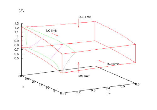
Figure 1: Solution space for the equilibrium models of the rotating magnetized stars. The $x$-, $y$-, and $z$-axis are the central density $\rho_{c}$, the magnetic field strength parameter $b$, and the axis ratio $r_{p}/r_{e}$, respectively. A point inside the cubic region drawn by the solid lines corresponds to a physically acceptable solution computed in this study. The sides of the cube labeled by “$B=0$ limit” “$\Omega=0$ limit” “MS limit” and “NC limit” represent the boundaries beyond which there is no physically acceptable solution. The surface labeled by “$B=0$ limit” corresponds to the non-magnetized limit, the surface labeled by “$\Omega=0$ limit” to the non-rotating limit, and the surface labeled by “MS limit” to the mass-shedding limit, and the surface labeled by “NC limit” to the non-convergence limit beyond which any solution cannot converge with the present numerical scheme. The surface embedded in the cube that is drawn with the dashed line boundary shows a set of equilibrium solutions having the same total baryon rest mass. The three dotted curves represent the constant magnetic flux sequences of equilibrium.

IV.1 Non-rotating models

First let us consider the static configurations for the following two reasons. (1) Since the magnetars and the high field neutron stars observed so far are all slow rotators, the static models could well approximate to such stars. (2) In the static models, one can see purely magnetic effects on the equilibrium properties because there is no centrifugal force and all the stellar deformation is attributed to the magnetic stress. In Fig. 2, we show distributions of the rest mass density and the magnetic field in the meridional planes for the two static equilibrium stars characterized by (1) $\rho_{c}=6.7\times 10^{14}[{\rm g/cm^{3}}]$, $M=1.46M_{\odot}$, $R_{\rm cir}=20.9{\rm km}$, $r_{p}/r_{e}=1.15$, $\bar{e}=-0.81$, $H/|W|=0.19$, and $k=1$, [Panels (a) and (c)] and by (2) $\rho_{c}=6.7\times 10^{14}[{\rm g/cm^{3}}]$, $M=1.51M_{\odot}$, $R_{\rm cir}=18.0{\rm km}$, $r_{p}/r_{e}=1.14$, $\bar{e}=-0.55$, $H/|W|=0.15$, and $k=2$ [Panels (b) and (d)]. These two models have the same maximum magnetic field strength of $5.0\times 10^{17}{\rm G}$. In Fig. 2, as mentioned, we can confirm that the magnetic stress due to the purely toroidal field makes the stellar shape prolate. This is a great contrast to the magnetic stress due to the purely poloidal field, for which the shape of the star deforms oblately as shown in Ref. (Chandra:1953, ). As for the dependence of $k$ on the stellar structures, it is found that the density distributions of the stars with $k=1$ are prolately more concentrated around the magnetic axis than those of the stars with $k=2$, as can be seen in Fig. 2. This feature is due to the magnetic pressure distributions. As mentioned in the Introduction, the toroidal magnetic field lines behave like a rubber belt that is wrapped around the waist of the stars. For the $k=1$ case, this tightening due to the toroidal fields is effective even near the surface of the star. To see it clearly, in Fig. 3, we give the ratio of the magnetic pressure to the matter pressure as functions of $r$ for the two models shown in Fig. 2. In this figure, we see that for the $k=1$ case, the magnetic pressure dominates over the matter pressure near the stellar surface, while for the $k=2$ case, the matter pressure dominates over the magnetic pressure there.

In Fig. 4, we show the gravitational mass $M$ of static models for several equilibrium sequences of constant $\Phi$ and of constant $M_{0}$ as functions of the central density $\rho_{c}$. Here, $\Phi_{22}$ means the flux normalized by units of $10^{22}$Weber, which is a typical value of the magnetic flux for a canonical neutron star model. In this figure, the curves labeled by their values of $M_{0}$ ($\Phi_{22}$) indicate the equilibrium sequence along which the values of $M_{0}$ ($\Phi_{22}$) are held constant. The filled circles in Fig. 4 indicate the maximum mass models of the equilibrium sequences of constant $\Phi$. The global physical quantities of these maximum mass models, the magnetic flux $\Phi_{22}$, the central baryon mass density $\rho_{c}$, the gravitational mass $M$, the baryon rest mass $M_{0}$, the circumferential radius at the equator $R_{\text{cir}}$, the maximum strength of the magnetic fields $B_{\text{max}}$, the ratio of the magnetic energy to the gravitational energy $H/|W|$, and the mean deformation rate $\bar{e}$ are summarized in Table 1. Form this table, we see that the strong toroidal magnetic fields of $10^{18}$ G make, roughly $15\%$ increase in the maximum gravitational mass of the stars and the highly prolate stellar deformation of $\bar{e}\approx-0.7$, even though the magnetic field of $10^{18}$ G might be too strong even for a magnetar model. The properties of the constant $M_{0}$ sequences will be discussed in detail later.

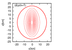
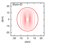
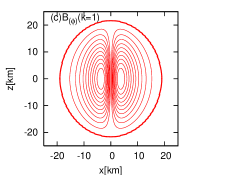
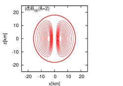
Figure 2: Distributions of the rest mass density and the magnetic field for the non-rotating magnetized stars whose maximum magnetic field strength is $5.0\times 10^{17}{\rm G}$. (a) Equi-rest-mass-density contours and (c) equi-$B_{(\phi)}$ contours in the meridional cross section for the $M=1.46M_{\odot}$, $R_{\rm cir}=20.9{\rm km}$, $H/|W|=0.19$, and $k=1$ model. (b) Equi-rest-mass-density contours and (d) equi-$B_{(\phi)}$ contours in the meridional cross section for the $M=1.51M_{\odot}$, $R_{\rm cir}=18.0{\rm km}$, $H/|W|=0.15$, and $k=2$ model. Thick ellipses denote the stellar surface.

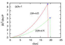
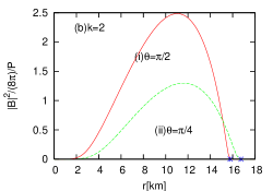
Figure 3: Ratio of the magnetic pressure to the matter pressure $|B|^{2}/(8\pi P)$ at the $\theta=\pi/2$ surfaces (solid lines) and the $\theta=\pi/4$ surfaces (dashed lines) for the models given in Fig. 2, given as functions of $r$. (a) $k=1$ and (b) $k=2$. The asterisks indicate the stellar surface.

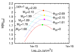
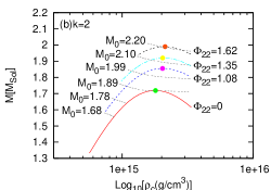
Figure 4: Central baryon mass density $\rho_{c}$ versus gravitational mass $M$ along the constant magnetic flux equilibrium sequences and the constant magnetic flux equilibrium sequences for the non-rotating stars. (a) $k=1$ and (b) $k=2$. The filled circles indicate the maximum gravitational mass models whose global physical quantities are given in Table 1. Each equilibrium sequence is labeled by its value for $M_{0}$ or $\Phi_{22}$.

Table 1: Global physical quantities for the maximum gravitational mass models of the constant magnetic flux sequences of the non-rotating stars.

$\Phi[10^{22}{\rm Weber}]$	$\rho_{c}[10^{15}{\rm g}/{\rm cm}^{3}]$	$M[M_{\rm\odot}]$	$M_{0}[M_{\rm\odot}]$	$R_{\text{cir}}[{\rm km}]$	$B_{\text{max}}[10^{18}{\rm G}]$	$H/|W|$	$\bar{e}$
k=1
0.000E+00	1.797E+00	1.719E+00	1.888E+00	1.180E+01	0.000E+00	0.000E+00	0.000E+00
1.616E+00	2.032E+00	1.843E+00	2.014E+00	1.457E+01	1.008E+00	1.253E-01	-4.284E-01
2.155E+00	2.026E+00	1.935E+00	2.107E+00	1.667E+01	1.129E+00	1.737E-01	-6.933E-01
2.694E+00	1.914E+00	2.041E+00	2.210E+00	1.951E+01	1.168E+00	2.186E-01	-1.012E+00
k=2
0.000E+00	1.797E+00	1.719E+00	1.888E+00	1.180E+01	0.000E+00	0.000E+00	0.000E+00
1.077E+00	2.032E+00	1.855E+00	2.055E+00	1.361E+01	8.023E-01	8.068E-02	-3.874E-01
1.347E+00	2.039E+00	1.920E+00	2.128E+00	1.444E+01	8.630E-01	1.024E-01	-5.315E-01
1.616E+00	2.126E+00	1.990E+00	2.210E+00	1.516E+01	9.205E-01	1.198E-01	-6.721E-01

IV.2 Rotating models

Next, let us move on to the rotation models. For the static stars with the purely toroidal magnetic field, as shown in the last subsection, the ratio of the magnetic energy to the gravitational energy $H/|W|$ can be of an order of $10^{-1}$, which is larger than a typical value of the ratio of the rotation energy to the gravitational energy $T/|W|$ for the rotating non-magnetized neutron star models. As shown in Komatsu:1989 , a typical value of $T/|W|$ for the uniformly rotating $n=1$ polytropic neutron star models having no magnetic field is of an order of $10^{-2}$. This fact implies that a large amount of the magnetic energy can be stored in the neutron star with infinite conductivity because the mass-shedding like limit does not appear for the magnetic force unlike the centrifugal force of the rotating star cases as argued in  Cardall:2001 . In this paper, as mentioned, we are concerned with equilibrium properties of the strongly magnetized stars. Thus, most stellar models treated here are magnetic-field-dominated ones in the sense that $H/|W|$ is larger than $T/|W|$ even for the mass-shedding models. In such models, the effects of the rotation on the stellar structures are necessarily supplementary and the basic properties do not highly depend on the rotation parameter.

In Fig. 5, we display the typical distributions of the rest mass density and the magnetic field for the two rotating equilibrium stars characterized by (1) $\rho_{c}=6.7\times 10^{14}[{\rm g/cm^{3}}]$, $M=1.53M_{\odot}$, $R_{\rm cir}=25.3{\rm km}$, $r_{p}/r_{e}=0.75$, $\bar{e}=-0.24$, $H/|W|=0.15$, $T/|W|=3.7\times 10^{-2}$, and $k=1$, [Panels (a) and (c)] and by (2) $\rho_{c}=6.7\times 10^{14}[{\rm g/cm^{3}}]$, $M=1.59M_{\odot}$, $R_{\rm cir}=21.2{\rm km}$, $r_{p}/r_{e}=0.78$, $\bar{e}=-6.9\times 10^{-2}$, $H/|W|=0.12$, $T/|W|=5.07\times 10^{-2}$, and $k=2$ [Panels (b) and (d)]. These models have the same maximum magnetic field strength of $4.5\times 10^{17}{\rm G}$. Comparing Fig. 5 with Fig. 2, we see that basic properties of the structures of the rotating models are similar to those of the static models. Difference between them only appears near the equatorial surface of the stars. As shown in Fig. 5, the density distributions are stretched from the rotation axis outward due to the centrifugal force and the shape of the stellar surface becomes oblate, which can be seen from the values of the axis ratio $r_{p}/r_{e}$. On the other hand, the equi-density contours deep inside the stars are oblate, which can be confirmed from the values of the mean deformation rate $\bar{e}$. This is because the centrifugal force is the most significant agent deforming the stars near the equatorial surface of the star since, as shown in equation (33), the anisotropic magnetic stress of the present models vanishes at the surface of the star.

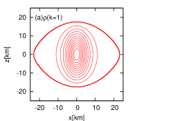
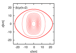
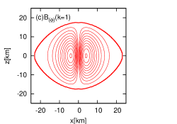
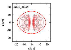
Figure 5: Distributions of the rest mass density and the magnetic field for the rotating magnetized stars whose maximum magnetic field strength is $4.5\times 10^{17}{\rm G}$. (a) Equi-rest-mass-density contours and (c) equi-$B_{(\phi)}$ contours in the meridional cross section for the $M=1.53M_{\odot}$, $R_{\rm cir}=25.3{\rm km}$, $H/|W|=0.15$, $T/|W|=3.7\times 10^{-2}$ , and $k=1$ model. (b) Equi-rest-mass-density contours and (d) equi-$B_{(\phi)}$ contours in the meridional cross section for the $M=1.59M_{\odot}$, $R_{\rm cir}=21.2{\rm km}$, $H/|W|=0.12$, $T/|W|=5.07\times 10^{-2}$, , and $k=2$ model. Thick ellipses denote the stellar surface.

IV.3 Constant baryon mass sequence

In this subsection, we concentrate on the constant baryon mass sequences of the magnetized stars. In the static star cases, this condition of the constant baryon mass picks out a single sequence of the equilibrium stars. Along such an equilibrium sequence, as mentioned, the magnetic flux of the stars cannot be held constant. For the rotating star cases, on the other hand, we can select a single sequence of the equilibrium stars by keeping the baryon rest mass and the magnetic flux constant simultaneously. The equilibrium sequences along which the baryon rest mass and the magnetic flux are conserved may model the isolated neutron stars that are adiabatically losing angular momentum via the gravitational radiation. It should be noted that here, we have omitted evolution of the function $K$, which will change its function form during such a process of losing angular momentum even though there has been no way to determine it so far. Thus, the constant baryon mass sequences considered in this study might be oversimplified for investigations of the adiabatic evolution of the isolated neutron stars. However, the inclusion of the evolution effects of the function $K$ is beyond the scope of the present study.

First we consider the constant baryon mass sequences of the non-rotating stars to clearly understand the basic properties of the simplest equilibrium sequences. Then we move on to the rotating cases. As done in Ref. Cook:1992 , we divide the equilibrium sequences of the magnetized stars into two classes, normal and supramassive equilibrium sequences. In this study, the normal (supramassive) equilibrium sequence is defined as an equilibrium sequence whose baryon rest mass is smaller (larger) than the maximum baryon rest mass of the non-magnetized and non-rotating stars. As shown in Fig. 4, the maximum baryon rest mass of the non-rotating and non-magnetized stars for the present EOS is given by $M_{0}=1.89M_{\odot}$. Therefore, the normal (supramassive) equilibrium sequences are simply defined as equilibrium sequences with $M_{0}<1.89M_{\odot}$ ($M_{0}>1.89M_{\odot}$).

IV.3.1 Static cases

In Fig. 4, one can see how the constant baryon mass sequences of the non-rotating stars are drawn on the $\rho_{c}$–$M$ plane. In this figure, the two constant baryon mass sequences characterized by $M_{0}=1.68M_{\odot}$ and $1.78M_{\odot}$ refer to the normal equilibrium sequences, while the three constant baryon mass sequences characterized by $M_{0}=1.99M_{\odot}$, $2.10M_{\odot}$, and $2.20M_{\odot}$ refer to the supramassive equilibrium sequences. In Fig. 4, one can confirm that the two normal equilibrium sequences of $M_{0}=1.68M_{\odot}$ and $1.78M_{\odot}$ indeed end at the equilibrium stars having $\Phi=0$ (no magnetic field) and that the supramassive equilibrium sequences never intersect with the curves given by $\Phi=0$. Note that all the end points of the equilibrium sequences of the non-rotating magnetized stars correspond to the “NC limit” in Fig. 1.

In Figs. 6 and 7, the global physical quantities, $\Delta M$, $\Delta R_{cir}$, $\Delta\rho_{c}$, and $\bar{e}$ are given as functions of the maximum values of $|B|$ inside the star, $B_{\rm max}$, for the normal equilibrium sequences with $M_{0}=1.68M_{\odot}$ and for the supramassive equilibrium sequences with $M_{0}=2.10M_{\odot}$, respectively. In these figures,

$$\Delta Q(B_{\rm max},M_{0})\equiv{Q(B_{\rm max},M_{0})-Q(|B|=0,M_{0})\over Q(|B|=0,M_{0})}\,,$$ (53)

where $Q$ stands for a physical quantity for the constant baryon mass sequences of the non-rotating stars. Numerical values of the global physical quantities, the magnetic flux $\Phi$, the central rest mass density $\rho_{c}$, the gravitational mass $M$, the circumferential radius $R_{\text{cir}}$, the maximum strength of the magnetic field $B_{\text{max}}$, the ratio of the magnetic energy to the gravitational energy $H/|W|$, and the mean deformation rate $\bar{e}$, for the selected models, which are displayed in Figs. 6 and 7, are also summarized in Tables 2 and  3. From Figs. 6 and 7, we see that, qualitatively, basic behavior of $\Delta M$, $\Delta R_{cir}$, $\Delta\rho_{c}$, $\bar{e}$ does not highly depend on the value of $k$. Comparing Fig. 6 with Fig. 7, we find that as the value of $B_{\rm max}$ is varied, the global changes in the global physical quantities for the normal sequences are of opposite directions to those for the supramassive equilibrium sequences.

Before going to the the rotating cases, in which we consider the equilibrium sequences along which the baryon rest mass and the magnetic flux are held constants, it is useful to investigate non-rotating solutions referred to these equilibrium sequences of the constant baryon rest mass and magnetic flux. Plots given in Fig. 4 tell us the number of such solutions. If the values of the baryon rest mass and magnetic flux are specified, one can pick out two curves corresponding to the constant baryon rest mass and the constant magnetic flux. Then, the intersections of these two curves indicate the members of the constant baryon rest mass and magnetic flux sequences in the non-rotating limit. For the solutions of the normal equilibrium sequences, characterized by $M_{0}<1.89$, it can be seen that there is a single intersection of the two curves. (Note that we only consider the solutions in the lower central density region, even though there are other solutions in the higher central density region.) For example, in the left panel of Fig. 4, the $M_{0}=1.78$ curve intersects once to the $\Phi_{22}=1.61$ curve. For the solutions of the supramassive equilibrium sequences, characterized by $M_{0}>1.89$, on the other hand, we see that there are the following three possibilities. (1) There is no intersection between the two curves, showing that the non-rotating limit does not exist. (2) There is a single intersection between the two curves, which is only possible when one curve is tangent to the other. In this case, a unique limit of no rotation exists. (3) There are two intersections between the two curves, showing that there are two different limits of no rotation in this case. For example, in the left panel of Fig. 4, let us consider the constant baryon rest mass sequence of $M_{0}=2.10$. If we chose $\Phi_{22}$ to be $2.15$, $2.05$, and $1.61$, then the numbers of the intersection of the two curves are, respectively, two, one, and zero, as can be seen from Fig. 4. Thus, it is found that the supramassive equilibrium sequences with $(M_{0},\ \Phi_{22})=(2.10,\ 1.61)$, $(2.10,\ 2.05)$, and $(2.10,\ 2.15)$ have no non-rotation limit, the single non-rotating limit, and double non-rotation limits, respectively. One important consequence of this fact is that there are two disconnected branches of the equilibrium sequences characterized by the same baryon rest mass and the magnetic flux for some supramassive equilibrium sequences, as discussed in the next subsection.

Table 2: Global physical quantities for the normal equilibrium sequences of the non-rotating stars with $M_{0}=1.68M_{\odot}$.

$\Phi[10^{22}{\rm Weber}]$	$\rho_{c}[10^{15}{\rm g}/{\rm cm}^{3}]$	$M[M_{\rm\odot}]$	$R_{\text{cir}}[{\rm km}]$	$B_{\text{max}}[10^{18}{\rm G}]$	$H/|W|$	$\bar{e}$
$k=1$
0.000E+00	8.569E-01	1.551E+00	1.430E+01	0.000E+00	0.000E+00	0.000E+00
1.171E+00	8.538E-01	1.576E+00	1.786E+01	5.222E-01	1.307E-01	-4.975E-01
1.754E+00	7.371E-01	1.600E+00	2.340E+01	5.458E-01	2.225E-01	-1.151E+00
2.120E+00	6.400E-01	1.614E+00	2.885E+01	5.111E-01	2.772E-01	-1.758E+00
$k=2$
0.000E+00	8.569E-01	1.551E+00	1.430E+01	0.000E+00	0.000E+00	0.000E+00
7.239E-01	8.178E-01	1.566E+00	1.611E+01	4.761E-01	8.635E-02	-3.372E-01
9.424E-01	7.677E-01	1.575E+00	1.735E+01	5.089E-01	1.232E-01	-5.391E-01
1.074E+00	7.335E-01	1.580E+00	1.825E+01	5.170E-01	1.454E-01	-6.831E-01

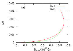
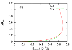
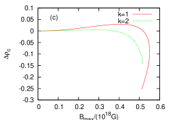
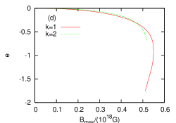
Figure 6: Global physical quantities (a) the change rate of the gravitational mass $\Delta M$, (b) the change rate of the circumferential radius at the equator $\Delta R_{\rm cir}$, (c) the change rate of the central rest mass density $\Delta\rho_{c}$, and (d) the mean deformation rate $\bar{e}$ along the normal equilibrium sequences of the non-rotating stars characterized by $M_{0}=1.68M_{\odot}$, given as functions of $B_{\rm max}$.

Table 3: Global physical quantities for the supramassive equilibrium sequences of the non-rotating stars with $M_{0}=2.10M_{\odot}$.

$\Phi[10^{22}{\rm Weber}]$	$\rho_{c}[10^{15}{\rm g}/{\rm cm}^{3}]$	$M[M_{\rm\odot}]$	$R_{\text{cir}}[{\rm km}]$	$B_{\text{max}}[10^{18}{\rm G}]$	$H/|W|$	$\bar{e}$
$k=1$
2.178E+00	1.779E+00	1.936E+00	1.765E+01	1.048E+00	1.842E-01	-7.650E-01
2.430E+00	1.415E+00	1.958E+00	2.083E+01	9.368E-01	2.230E-01	-1.064E+00
2.650E+00	1.222E+00	1.974E+00	2.374E+01	8.659E-01	2.532E-01	-1.351E+00
2.838E+00	1.092E+00	1.987E+00	2.651E+01	8.102E-01	2.778E-01	-1.626E+00
$k=2$
1.250E+00	1.980E+00	1.896E+00	1.424E+01	8.360E-01	9.620E-02	-4.833E-01
1.365E+00	1.625E+00	1.909E+00	1.542E+01	8.044E-01	1.162E-01	-5.874E-01
1.460E+00	1.468E+00	1.918E+00	1.622E+01	7.897E-01	1.307E-01	-6.753E-01
1.538E+00	1.371E+00	1.925E+00	1.685E+01	7.793E-01	1.421E-01	-7.510E-01

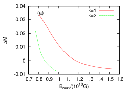
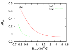
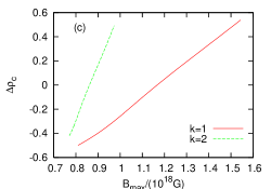
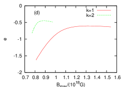
Figure 7: Same as Fig. 6, but for the supramassive sequence with $M_{0}=2.10M_{\odot}$.

IV.3.2 Rotating cases

First, let us consider the normal equilibrium sequences of the magnetized rotating stars. In Figs. 8 and 9, we show the global physical quantities $M$, $R_{cir}$, $\rho_{c}$, $J$, $B_{\rm max}$, and $\bar{e}$ as functions of $\Omega$ for the constant baryon mass and magnetic flux equilibrium sequences with $k=1$ and $k=2$, respectively. All the equilibrium sequences given in these figures are of the normal equilibrium sequences characterized by the constant baryon rest mass given by $M_{0}=1.78M_{\odot}$. In Figs. 8 and 9, each curve is labeled by its value of $\Phi_{22}$ which is held constant along the equilibrium sequence. For the sake of comparison, the physical quantities for the non-magnetized equilibrium sequences ($\Phi_{22}=0$) are also given in Figs. 8 and 9. Note that the constant baryon rest mass equilibrium sequences of the non-magnetized polytropic stars have been argued in detail in Ref. Cook:1992 . Numerical values of the global physical quantities, the central rest mass density $\rho_{c}$, the gravitational mass $M$, the circumferential radius $R_{\text{cir}}$, the angular velocity $\Omega$, the angular momentum $J$, the ratio of the rotation energy to the gravitational energy $T/|W|$, the ratio of the magnetic energy to the gravitational energy $H/|W|$, the mean deformation rate $\bar{e}$, and the maximum strength of the magnetic field $B_{\text{max}}$, for some selected models are tabulated in Tables 4 and 5 for the cases of $k=1$ and $k=2$, respectively.

In Figs. 8 and 9, as discussed, we see that all the normal equilibrium sequences begin at the non-rotating equilibrium stars and continue to the mass-shedding limits, at which the sequences end, as the angular velocity increases. (In Figs. 8 and 9, the asterisks indicate the mass-shedding models.) It is also found from these figures that the behavior of the normal equilibrium sequences as functions of $\Omega$ are basically independent of the values of $\Phi_{22}$ and $k$. As the angular velocity is increased, the gravitational masses and the circumferential radii increase, while the central densities and the maximum strength of the magnetic fields decrease because of the baryon rest mass constancy and of the magnetic flux constancy, respectively. The angular momenta are monotonically increasing functions of the angular velocity, which implies that the angular momentum loss via gravitational radiation results in the spin down of the star for the normal equilibrium sequences.

Table 4: Global physical quantities for the normal equilibrium sequences of the rotating stars with $M_{0}=1.78M_{\odot}$ and $k=1$.

$\rho_{c}[10^{15}{\rm g}/{\rm cm}^{3}]$	$M[M_{\rm\odot}]$	$R_{\text{cir}}[{\rm km}]$	$\Omega[10^{3}{\rm rad/s}]$	$cJ/GM_{\odot}^{2}$	$T/|W|$	$H/|W|$	$\bar{e}$	$B_{\text{max}}[10^{17}{\rm G}]$
$\Phi_{22}=0$
5.745E-01	1.666E+00	2.235E+01	4.571E+00	1.905E+00	9.657E-02	0.000E+00	2.636E-01	0.000E+00
6.286E-01	1.661E+00	1.925E+01	4.552E+00	1.707E+00	8.224E-02	0.000E+00	2.310E-01	0.000E+00
7.864E-01	1.650E+00	1.616E+01	4.008E+00	1.179E+00	4.497E-02	0.000E+00	1.368E-01	0.000E+00
8.987E-01	1.644E+00	1.490E+01	3.230E+00	8.355E-01	2.444E-02	0.000E+00	7.764E-02	0.000E+00
1.073E+00	1.637E+00	1.356E+01	0.000E+00	0.000E+00	0.000E+00	0.000E+00	1.928E-04	0.000E+00
$\Phi_{22}=1.14$
8.261E-01	1.674E+00	2.542E+01	3.627E+00	1.131E+00	4.242E-02	1.194E-01	-1.697E-01	4.957E+00
8.739E-01	1.670E+00	2.065E+01	3.386E+00	9.709E-01	3.279E-02	1.180E-01	-2.053E-01	5.162E+00
9.017E-01	1.668E+00	1.952E+01	3.154E+00	8.631E-01	2.663E-02	1.170E-01	-2.395E-01	5.275E+00
9.913E-01	1.663E+00	1.732E+01	2.035E+00	4.937E-01	9.463E-03	1.133E-01	-3.339E-01	5.621E+00
1.044E+00	1.660E+00	1.642E+01	0.000E+00	0.000E+00	0.000E+00	1.111E-01	-3.883E-01	5.809E+00
$\Phi_{22}=1.71$
7.947E-01	1.692E+00	3.202E+01	2.554E+00	8.514E-01	2.516E-02	2.001E-01	-6.485E-01	5.671E+00
8.314E-01	1.689E+00	2.482E+01	2.227E+00	6.776E-01	1.690E-02	1.988E-01	-7.263E-01	5.871E+00
8.504E-01	1.687E+00	2.340E+01	1.957E+00	5.703E-01	1.230E-02	1.979E-01	-7.791E-01	5.977E+00
8.782E-01	1.686E+00	2.200E+01	1.453E+00	4.019E-01	6.310E-03	1.973E-01	-8.298E-01	6.125E+00
9.035E-01	1.684E+00	2.084E+01	0.000E+00	0.000E+00	0.000E+00	1.959E-01	-9.042E-01	6.258E+00

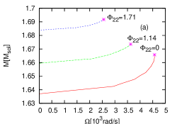
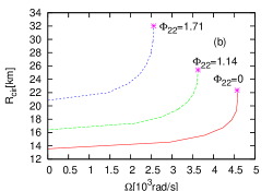
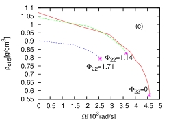
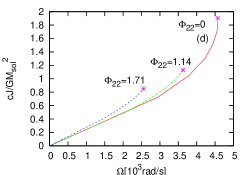
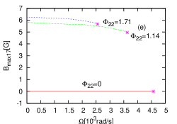
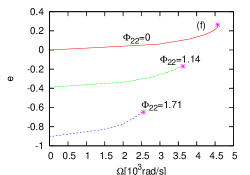
Figure 8: Global physical quantities $M$, $R_{cir}$, $\rho_{c}$, $J$, $B_{\rm max}$, and $\bar{e}$ for the constant baryon mass and magnetic flux equilibrium sequences with $k=1$, given as functions of $\Omega$. All the equilibrium sequences are referred to the normal equilibrium sequences characterized by the constant baryon rest mass $M_{0}=1.78M_{\odot}$. Each sequence is labeled by its value of $\Phi_{22}$. The asterisks indicate the mass-shedding models.

Table 5: Global physical quantities for the normal equilibrium sequences of the rotating stars with $M_{0}=1.78M_{\odot}$ and $k=2$.

$\rho_{c}[10^{15}{\rm g}/{\rm cm}^{3}]$	$M[M_{\rm\odot}]$	$R_{\text{cir}}[{\rm km}]$	$\Omega[10^{3}{\rm rad/s}]$	$cJ/GM_{\odot}^{2}$	$T/|W|$	$H/|W|$	$\bar{e}$	$B_{\text{max}}[10^{17}{\rm G}]$
$\Phi_{22}=0.60$
6.943E-01	1.668E+00	2.327E+01	4.191E+00	1.511E+00	6.772E-02	6.524E-02	6.091E-02	3.842E+00
7.115E-01	1.667E+00	2.133E+01	4.185E+00	1.464E+00	6.459E-02	6.483E-02	6.430E-02	3.898E+00
8.137E-01	1.658E+00	1.769E+01	3.742E+00	1.083E+00	3.949E-02	6.203E-02	-4.386E-02	4.245E+00
9.465E-01	1.650E+00	1.562E+01	2.503E+00	6.106E-01	1.373E-02	5.869E-02	-1.449E-01	4.617E+00
1.024E+00	1.646E+00	1.475E+01	0.000E+00	0.000E+00	0.000E+00	5.666E-02	-2.079E-01	4.837E+00
$\Phi_{22}=0.95$
7.757E-01	1.670E+00	1.979E+01	3.156E+00	9.639E-01	3.195E-02	1.165E-01	-2.838E-01	5.052E+00
8.181E-01	1.667E+00	1.863E+01	2.811E+00	8.000E-01	2.291E-02	1.150E-01	-3.297E-01	5.222E+00
8.710E-01	1.663E+00	1.745E+01	2.112E+00	5.532E-01	1.146E-02	1.130E-01	-3.955E-01	5.428E+00
9.001E-01	1.661E+00	1.684E+01	7.827E-01	2.024E-01	4.036E-03	1.118E-01	-4.507E-01	5.541E+00
9.198E-01	1.659E+00	1.651E+01	0.000E+00	0.000E+00	0.000E+00	1.109E-01	-4.785E-01	5.607E+00

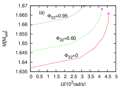
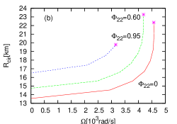
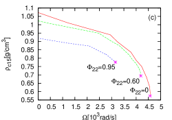
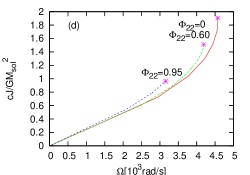
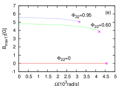
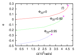
Figure 9: Same as Fig. 8, but for $k=2$.

Now consider the supramassive equilibrium sequences of the magnetized rotating stars. Figures 10 and 11 give the plots of the global physical quantities $M$, $R_{\text{cir}}$, $\rho_{c}$, $J$, $B_{\rm max}$, and $\bar{e}$ as functions of $\Omega$ for the constant baryon mass and magnetic flux equilibrium sequences with $k=1$ and $k=2$, respectively. All the equilibrium sequences given in these figures are of the supramassive equilibrium sequences characterized by the constant baryon rest mass given by $M_{0}=2.10M_{\odot}$. In Figs. 10 and 11, each curve is labeled by its value of $\Phi_{22}$ which is held constant along the equilibrium sequence. For the sake of comparison, the physical quantities for the non-magnetized equilibrium sequences ($\Phi_{22}=0$) are also given in Figs. 10 and 11. Numerical values of the global physical quantities, $\rho_{c}$, $M$, $R_{\text{cir}}$, $\Omega$, $J$, $T/|W|$, $H/|W|$, $\bar{e}$, and $B_{\text{max}}$, for some selected models are summarized in Tables 6 and 7 for the cases of $k=1$ and $k=2$, respectively.

In Figs. 10 and 11, we show the two different types of the supramassive sequences, as argued before. One is the equilibrium sequence that does not connect to the non-rotating solutions, whose examples correspond to the sequences labeled by $\Phi_{22}=1.42$ for the $k=1$ case and by $\Phi_{22}=0.80$ for the $k=2$ case. In this type of the equilibrium sequences, the sequences begin at the mass-shedding limits with lower central density $\rho_{c}$ and move to other mass-shedding limits with higher central density $\rho_{c}$ as the angular velocity $\Omega$ increases. This feature is the same as that of the supramassive equilibrium sequences of non-magnetized stars (see, e.g., Ref. Cook:1992 ). The other is the equilibrium sequence composed of two disconnected sequences that begin at two different non-rotating stars and move to the mass-shedding limits as the angular velocity increases. This type of equilibrium sequences does not appear in the non-magnetized stars, in which all the equilibrium sequences have a single limit of no rotation as long as it exits. This type of the equilibrium sequences corresponds to the sequences labeled by $\Phi_{22}=2.13$ for the $k=1$ case and by $\Phi_{22}=1.28$ for the $k=2$ case. The basic behavior of the global physical quantities for the supramassive sequences is nearly independent of $\Phi_{22}$ and $k$ if we do not consider the equilibrium sequences composed of two disconnected sequences.

In Fig. 12, we show the solution space for the equilibrium models of the rotating magnetized stars (similar to Fig. 1, in which some normal equilibrium sequences are given) in order to clearly understand the properties of the supramassive equilibrium sequences. In Fig. 12, a point inside the cubic region drawn by the solid lines again corresponds to a physically acceptable solution computed in this study, and the surface drawn with the dashed curve boundary shows a set of the supramassive solutions characterized by the baryon rest mass $M_{0}=2.10M_{\odot}$. In this figure, the three dotted curves indicate the three equilibrium sequences of the constant baryon rest mass and magnetic flux characterized by $\Phi_{22}=2.13$, $1.42$, and $0$. In Fig. 12, we see that the two sequences with $\Phi_{22}=0\ {\rm and}\ 1.14$ do not have a non-rotating limit and terminate at the mass-shedding limits and that the sequence with $\Phi_{22}=1.71$ is composed of the two disconnected equilibrium sequences beginning at the non-rotating limits and terminating at the mass-shedding limits. (Compare with the plots for the normal sequences in Fig. 1).

Table 6: Global physical quantities for the supramassive equilibrium sequences of the rotating stars with $M_{0}=2.10M_{\odot}$ and $k=1$.

$\rho_{c}[10^{15}{\rm g}/{\rm cm}^{3}]$	$M[M_{\rm\odot}]$	$R_{\text{cir}}[{\rm km}]$	$\Omega[10^{3}{\rm rad/s}]$	$cJ/GM_{\odot}^{2}$	$T/|W|$	$H/|W|$	$\bar{e}$	$B_{\text{max}}[10^{17}{\rm G}]$
$\Phi_{22}=0$
9.817E-01	1.925E+00	1.945E+01	5.965E+00	2.312E+00	9.223E-02	0.000E+00	2.541E-01	0.000E+00
1.348E+00	1.913E+00	1.526E+01	6.383E+00	1.916E+00	6.952E-02	0.000E+00	1.991E-01	0.000E+00
1.797E+00	1.911E+00	1.387E+01	7.221E+00	1.831E+00	6.497E-02	0.000E+00	1.886E-01	0.000E+00
2.359E+00	1.918E+00	1.400E+01	8.775E+00	2.024E+00	7.646E-02	0.000E+00	2.242E-01	0.000E+00
2.421E+00	1.920E+00	1.460E+01	8.955E+00	2.055E+00	7.828E-02	0.000E+00	2.305E-01	0.000E+00
$\Phi_{22}=1.42$
1.692E+00	1.925E+00	2.072E+01	5.289E+00	1.434E+00	4.181E-02	1.076E-01	-8.604E-02	8.365E+00
1.797E+00	1.922E+00	1.849E+01	5.374E+00	1.395E+00	3.990E-02	1.053E-01	-8.439E-02	8.668E+00
2.247E+00	1.916E+00	1.686E+01	6.014E+00	1.385E+00	3.926E-02	9.679E-02	-5.343E-02	9.797E+00
2.327E+00	1.916E+00	1.693E+01	6.185E+00	1.406E+00	4.020E-02	9.542E-02	-4.119E-02	9.985E+00
2.461E+00	1.915E+00	1.807E+01	6.462E+00	1.444E+00	4.195E-02	9.325E-02	-2.345E-02	1.027E+01
$\Phi_{22}=2.13$
1.342E+00	1.955E+00	2.808E+01	3.336E+00	1.077E+00	2.441E-02	1.940E-01	-5.509E-01	8.626E+00
1.470E+00	1.948E+00	2.144E+01	2.977E+00	8.587E-01	1.635E-02	1.896E-01	-6.091E-01	9.183E+00
1.557E+00	1.944E+00	1.996E+01	2.649E+00	7.196E-01	1.175E-02	1.866E-01	-6.452E-01	9.539E+00
1.700E+00	1.938E+00	1.842E+01	2.035E+00	5.112E-01	6.072E-03	1.819E-01	-6.753E-01	1.010E+01
1.937E+00	1.930E+00	1.685E+01	0.000E+00	0.000E+00	0.000E+00	1.744E-01	-6.986E-01	1.095E+01
$\Omega=0$ Limit
2.495E+00	1.917E+00	1.535E+01	0.000E+00	0.000E+00	0.000E+00	1.597E-01	-6.066E-01	1.266E+01
2.841E+00	1.914E+00	1.522E+01	2.739E+00	5.283E-01	6.281E-03	1.526E-01	-4.973E-01	1.357E+01
3.080E+00	1.913E+00	1.542E+01	3.884E+00	7.404E-01	1.197E-02	1.483E-01	-4.133E-01	1.413E+01
3.366E+00	1.913E+00	1.618E+01	5.014E+00	9.548E-01	1.927E-02	1.437E-01	-3.114E-01	1.474E+01
3.370E+00	1.913E+00	1.621E+01	5.030E+00	9.579E-01	1.938E-02	1.436E-01	-3.098E-01	1.475E+01

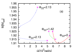
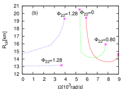
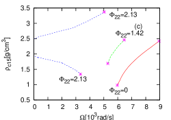
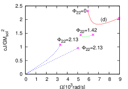
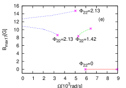
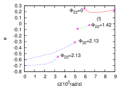
Figure 10: Global physical quantities $M$, $R_{cir}$, $\rho_{c}$, $J$, $B_{\rm max}$, and $\bar{e}$ for the constant baryon mass and magnetic flux equilibrium sequences with $k=1$, given as functions of $\Omega$. All the equilibrium sequences are referred to the supramassive equilibrium sequences characterized by the constant baryon rest mass $M_{0}=2.10M_{\odot}$. Each sequence is labeled by its value of $\Phi_{22}$. The asterisks indicate the mass-shedding models.

Table 7: Global physical quantities for the supramassive equilibrium sequences of the rotating stars with $M_{0}=2.10M_{\odot}$ and $k=2$.

$\rho_{c}[10^{15}{\rm g}/{\rm cm}^{3}]$	$M[M_{\rm\odot}]$	$R_{\text{cir}}[{\rm km}]$	$\Omega[10^{3}{\rm rad/s}]$	$cJ/GM_{\odot}^{2}$	$T/|W|$	$H/|W|$	$\bar{e}$	$B_{\text{max}}[10^{17}{\rm G}]$
$\Phi_{22}=0.80$
1.240E+00	1.923E+00	2.053E+01	5.362E+00	1.789E+00	6.045E-02	6.629E-02	3.648E-02	5.754E+00
1.590E+00	1.909E+00	1.607E+01	5.466E+00	1.477E+00	4.441E-02	5.989E-02	-9.328E-03	6.411E+00
2.022E+00	1.899E+00	1.461E+01	5.756E+00	1.343E+00	3.771E-02	5.365E-02	-3.089E-02	6.973E+00
2.520E+00	1.895E+00	1.417E+01	6.645E+00	1.417E+00	4.118E-02	4.831E-02	-8.473E-03	7.399E+00
3.038E+00	1.898E+00	1.593E+01	7.783E+00	1.619E+00	5.082E-02	4.427E-02	6.335E-02	7.682E+00
$\Phi_{22}=1.28$
1.227E+00	1.930E+00	1.931E+01	3.946E+00	1.266E+00	3.308E-02	1.202E-01	-3.038E-01	6.928E+00
1.367E+00	1.921E+00	1.750E+01	3.535E+00	1.012E+00	2.238E-02	1.158E-01	-3.693E-01	7.296E+00
1.558E+00	1.912E+00	1.601E+01	2.758E+00	7.021E-01	1.138E-02	1.101E-01	-4.344E-01	7.725E+00
1.601E+00	1.910E+00	1.577E+01	2.596E+00	6.453E-01	9.524E-03	1.089E-01	-4.455E-01	7.807E+00
1.833E+00	1.900E+00	1.464E+01	0.000E+00	0.000E+00	0.000E+00	1.026E-01	-5.142E-01	8.226E+00
$\Omega=0$ Limit
2.884E+00	1.879E+00	1.308E+01	0.000E+00	0.000E+00	0.000E+00	8.380E-02	-4.594E-01	9.282E+00
2.905E+00	1.879E+00	1.308E+01	1.231E-01	2.363E-02	3.539E-04	8.353E-02	-4.559E-01	9.293E+00
3.274E+00	1.878E+00	1.314E+01	3.102E+00	5.531E-01	7.964E-03	7.940E-02	-3.768E-01	9.478E+00
3.335E+00	1.878E+00	1.318E+01	3.665E+00	6.491E-01	9.419E-03	7.882E-02	-3.609E-01	9.504E+00

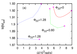
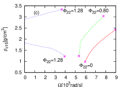
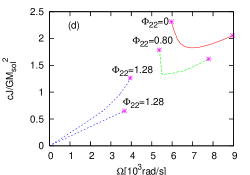
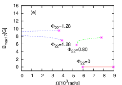
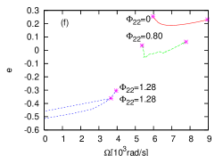
Figure 11: Same as Fig. 10, but for $k=2$.

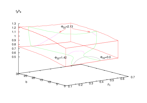
Figure 12: Same as Fig. 1, but the surface embedded in the cube that is drawn with the dashed line boundary shows a set of supramassive equilibrium solutions having the same total baryon rest mass. The three dotted curves represent the constant magnetic flux sequences referred to these supramassive equilibrium solutions.

V Discussion and Summary

V.1 Discussion

Important findings of the magnetic effects on the equilibrium properties in this study are summarized as follows ; (1) The mean deformation rates $\bar{e}$ for the strongly magnetized stars are basically negative, which means that the mean matter distributions are prolate, even when the stars rotate at the angular velocity of nearly the mass-shedding limits. (See, the panel (f) of Figs. 8 through 11.) This implies that rapidly rotating stars containing strong toroidal magnetic fields could wobble due to their prolate matter distributions and be potential sources of nearly periodic gravitational waves for large-scale gravitational wave detectors Cutler:2002nw . (2) The stronger toroidal magnetic fields lead the mass-shedding of the stars at the lower $\Omega$ or $T/|W|$. (See, Tables 4 through 7.) This is because the central concentration of the matter rises as the toroidal magnetic fields increase, as shown in Fig. 2. The larger central concentration of the matter then induces the mass-shedding at the lower $T/|W|$, as shown in the studies on the non-magnetized rotating stars (see, e.g., Refs.Komatsu:1989 ; Cook:1992 ).

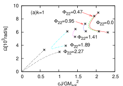
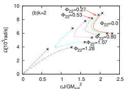
Figure 13: Angular velocity $\Omega$ for the supramassive equilibrium sequence of the rotating magnetized stars with $M_{0}=2.10M_{\odot}$, given as functions of the angular momentum $J$. (a) $k=1$ and (b) $k=2$. Each curve is labeled by its value of $\Phi_{22}$. The asterisks indicate the mass-shedding models.

One of the astrophysically important features of the constant baryon mass equilibrium sequences of the non-magnetized rotating stars is the spin up of the stars as the stellar angular momentum decreases, found by Shapiro et al. Shapiro:1990 (see, also, Ref. Cook:1992 ). This spin up effect of the relativistic stars containing purely poloidal magnetic fields has also been found in Bocquet:1995 . Now, let us investigate whether this spin up effect can occur for the rotating stars having purely toroidal magnetic fields, by examining the relationship between the angular velocity and the angular momentum of the stars. In Fig. 13, we show the angular velocity $\Omega$ as functions of the angular momentum $J$ for the supramassive equilibrium sequences characterized by the baryon rest mass $M_{0}=2.10M_{\odot}$. In this figure, the panels (a) and (b) give the plots for $k=1$ and $k=2$, respectively, and each curve is labeled by its value of $\Phi_{22}$, which is kept constant along the equilibrium sequence. In Fig. 13, the plots for the cases of $\Phi_{22}=0$ (the non-magnetized cases) are also shown. From these plots, we confirm that for the non-magnetized cases, the angular velocities increase as the angular momentum decreases, as shown in Cook:1992 . It can be also seen from this figure that similar spin up effects indeed occur for the equilibrium sequences characterized by $\Phi_{22}=0.47$, $0.95,$ and $1.41$ for the $k=1$ case and by $\Phi_{22}=0.27$, $0.53,$ for the $k=2$ case. The two equilibrium sequences with $\Phi_{22}=2.27$ for the $k=1$ case and with $\Phi_{22}=1.28$ for the $k=2$ case are special in the sense that these sequences have a cusp at the point of $(J,\ \Omega)=(0,\ 0)$. The one branch of these equilibrium sequences is seemingly continuous to the other branch. But, the two equilibrium stars having $(J,\ \Omega)=(0,\ 0)$ are totally different solutions as discussed before (see, also, Figs. 10 and 11). Thus, we have to treat these two branches as different equilibrium sequences because they are discontinuous at $(J,\ \Omega)=(0,\ 0)$. As a result, there is no spin up effect for such equilibrium sequences. For the other equilibrium sequences given in Fig. 13, on the other hand, we see that the star initially spins down as it loses angular momentum, and then it reaches the region of the spin up effects eventually.

Although, in this study, we employ the polytrope equation of state and simple functional forms of $K$, which determines the magnetic field distributions inside the star, the numerical scheme in this paper can be easily extended to treat more complicated functions for $K$ and realistic equations of state. To perform more quantitative investigations, we plan to explore the effects of realistic equations of state on the magnetized relativistic stars.

In this study, we assume the magnetic fields inside the star to be purely toroidal because we are concerned with the neutron stars whose the toroidal magnetic fields are much higher than the poloidal fields, which are likely to be produced in the core-collapse supernova, as suggested in some MHD simulations. However, this assumption of the purely toroidal magnetic fields oversimplifies the structures of the magnetized neutron stars because there will be poloidal magnetic fields in the neutron stars for the following two reasons ; (1) Seed poloidal magnetic fields and differential rotation are necessary to amplify the toroidal magnetic fields via the winding up mechanism. (2) It is likely that the neutron stars observed so far have poloidal magnetic fields, which will yield the spin down of the neutron stars via electromagnetic radiation. Therefore, we need to extend the present study to incorporate the effects of the poloidal magnetic fields in order to construct more realistic models of the magnetized neutron stars, which will be a very hard task. Note that similar extension within the framework of Newtonian dynamics has already been achieved Tomimura:2005 ; Yoshida:2006a ; Yoshida:2006b . The prime difficulty encountered is related to the treatment of the spacetime around the stars containing the mixed poloidal-toroidal magnetic fields. As discussed in Gourgoulhon:1993 , we cannot employ the simple metric (7) if the mixed poloidal-toroidal magnetic fields are considered. Instead, we have to use a metric whose non-zero components are increased in number and solve more complicated Einstein equations than those of the present study, which makes the problem intractable. As for the stability of the stars obtained here, which is beyond the scope of this article, some models obtained in this study might be unstable because the toroidal magnetic field with $k=1$ induces the kink instability near the magnetic axes as shown in the Newtonian analysis Tayler: 1973 . However, such instabilities are insignificant for the neutron star models if the growing timescales of the instabilities are much longer than the life-time of the stars. Therefore, we have to investigate the detailed properties of the stability of the stars by using linear perturbation analysis or numerical simulations to see whether or not such instabilities are indeed effective for the neutron star models. The two problems concerning the magnetized star models mentioned above, however, remain as future work of the greatest difficulty.

V.2 Summary

In this study, we have investigated the effects of the purely toroidal magnetic field on the equilibrium structures of the relativistic stars. The master equations for obtaining equilibrium solutions of relativistic rotating stars containing purely toroidal magnetic fields have been derived for the first time. In our formalism, the distribution of the magnetic fields are determined by an arbitrary function of $\rho_{0}hg_{B}$, $K(\rho_{0}hg_{B})$, which can be chosen freely as long as the boundary conditions for the magnetic fields on the magnetic axis and the surface of the star are satisfied. To solve these master equations numerically, we have extended the Cook-Shapiro-Teukolsky scheme for calculating relativistic rotating stars containing no magnetic field to incorporate the effects of the purely toroidal magnetic fields. By using the numerical scheme, we have then calculated a large number of the equilibrium configurations for particular function form of $K$ in order to explore the equilibrium properties. We have also constructed the equilibrium sequences of the constant baryon mass and/or the constant magnetic flux, which model the evolution of an isolated neutron star as it loses angular momentum via gravitational waves. Important properties of the equilibrium configurations of the magnetized stars obtained in this study are summarized as follows ; (1) For the non-rotating stars, the matter distribution of the stars is prolately distorted due to the toroidal magnetic fields. (2) For the rapidly rotating stars, on the other hand, the shape of the stellar surface becomes oblate because of the centrifugal force. But, the matter distribution deep inside the star is sufficiently prolate for the mean deformation rate $\bar{e}$ to be negative. Here, a negative value of $\bar{e}$ means that mean matter distribution is prolate. (3) The stronger toroidal magnetic fields lead to the mass-shedding of the stars at the lower $\Omega$ or $T/|W|$. (4) For some supramassive equilibrium sequences of the constant baryon mass and magnetic flux, the stars can spin up as they are losing angular momentum.

Appendix A Magnetic energy and flux for the star with purely toroidal magnetic fields

For the perfectly conductive fluid, the total energy-momentum four-vector $p^{\mu}$ measured by the observers with the matter four-velocity $u^{\mu}$ is given by

$$p^{\mu} = {T^{\mu}}_{\nu}u^{\nu}$$ (54)

$$= -\left(\rho_{0}+\rho_{0}e+\frac{1}{8\pi}\,B^{\alpha}B_{\alpha}\right)u^{\mu}\,.$$

Then, the total proper energy of the matter $E_{\rm proper}$ may be defined as

$$E_{\rm proper} = -\int p^{\mu}d^{3}\Sigma_{\mu}$$ (55)

$$= \int\left(\rho_{0}+\rho_{0}e+\frac{1}{8\pi}\,B^{\alpha}B_{\alpha}\right)u^{\mu}d^{3}\Sigma_{\mu}$$

$$= \int\left(\rho_{0}+\rho_{0}e+\frac{1}{8\pi}\,B^{\alpha}B_{\alpha}\right)u^{t}\sqrt{-g}\,d^{3}x\,.$$

We see that the first, the second, and the third term in the last line of equation (55) respectively represent the total baryon rest mass, the total internal energy, and the magnetic energy of the system. We may therefore define the stellar magnetic energy $H$ as

$$H=\frac{1}{8\pi}\,\int B^{\alpha}B_{\alpha}u^{t}\sqrt{-g}\,d^{3}x\,.$$ (56)

Next, let us consider the magnetic flux. Since the two conditions, given by

$$u^{\mu}F_{[\mu\nu,\alpha]}=0\,,$$ (57)

$$F_{\mu\nu}\,u^{\nu}=0\,,$$ (58)

are satisfied because of the Maxwell equation and infinite conductivity of the fluid, we have

$${\cal L}_{\alpha u}F_{\mu\nu}=0\,,$$ (59)

where ${\cal L}_{u}$ stands for the Lie differentiation with respect to $u^{\mu}$, and $\alpha$ denotes an arbitrary function. This implies that the flux of $F_{\mu\nu}$ is conserved along any tube generated by curves parallel to $u^{\mu}$. In other words, the integral of $F_{\mu\nu}$, defined as

$$\Phi=\int_{\Sigma(\tau)}F_{\mu\nu}\,dx^{\mu}\wedge dx^{\nu}\,,$$ (60)

where $\Sigma(\tau)$ is a two-dimensional surface co-moving with the fluid flow parametrized by its proper time $\tau$, is conserved in the sense that

$${d\Phi\over d\tau}=0\,.$$ (61)

In the present situation, we can take as $\Sigma(\tau)$ the two-surface orthogonal to the plane defined by the two Killing vectors parametrized by $r$ and $\theta$. For the present situation, we can then reduce $\Phi$ into

$$\Phi=\int^{\infty}_{0}dr\int^{\pi}_{0}d\theta\,F_{12}\,,$$ (62)

which is frequently called the magnetic flux.

References

- (1) Bocquet, M., Bonazzola, S., Gourgoulhon, E., & Novak, J. 1995, A&A, 301, 757
- (2) Bonazzola, S. & Gourgoulhon, E., 1994, CQG, 11, 1775
- (3) Bonazzola, S., & Gourgoulhon, E., 1996, A&A 312, 675
- (4) Cardall, C. Y., Prakash, M., & Lattimer, J. M. 2001 ApJ, 554, 322
- (5) Carter, B., 1969, J. Math. Phys. 10, 70
- (6) Chandrasekhar, S., & Fermi, E. 1953, ApJ 118, 116
- (7) Cook, G. B., Shapiro,S. L. & Teukolsky, S. A., ApJ 398, 203 (1992), 422, 227, (1994)
- (8) Cutler, C., 2002, PRD 66, 084025
- (9) Ferrario, L. & Wickramasinghe, D., 2007 MNRAS, 375, 1009
- (10) Geppert, U. and Rheinhardt, M. A& A, 456, 639
- (11) Gourgoulhon, E., & Bonazzola, S., 1993, PRD, 48, 2635
- (12) Gourgoulhon, E., & Bonazzola, S., 1994 CQG, 11, 443
- (13) Harding, A. K., & Lai, D. 2006, Reports of Progress in Physics, 69, 2631
- (14) Hachisu, I. 1986, ApJS, 61, 479
- (15) Ioka, K. & Sasaki, M. 2003, PRD 67, 124026
- (16) Ioka, K. & Sasaki, M. 2004, ApJ 600, 296
- (17) Kiuchi, K., & Kotake, K., appeared in MNRAS, arXiv:0708.3597 [astro-ph].
- (18) Komatsu, H., Eriguchi, Y., & Hachisu, I., MNRAS, 237, 355 (1989), 239, 153 (1989)
- (19) Konno, K., Obata, T.& Kojima, Y. 1999, A&A, 352, 211
- (20) Kotake, K., Sawai, H., Yamada, S., & Sato, K. 2004, ApJ, 608, 391
- (21) Kotake, K., Sato, K., & Takahashi, K. 2006, Reports of Progress in Physics, 69, 971
- (22) Kouveliotou, C., et al. 1998, Nature, 393, 235
- (23) Lattimer, J. M. & Prakash, M. 2006 astro-ph/0612440.
- (24) Livne, E., Dessart, L., Burrows, A., & Meakin, C. A. 2007, ApJS, 170, 187
- (25) Miketinac, M. J. 1973 Ap&SS, 22, 413
- (26) Moiseenko, S. G., Bisnovatyi-Kogan, G. S., & Ardeljan, N. V. 2006, MNRAS, 370, 501
- (27) Obergaulinger, M., Aloy, M. A., Müller, E. 2006, A&A, 450, 1107
- (28) Oron, A., 2002, PRD, 66, 023006
- (29) Shapiro, S. L., Teukolsky, S.A., & Nakamura, T. 1990, ApJ, 357, L17
- (30) Shibata, M., Taniguchi, K., & Uryu, K., 2005, PRD 71, 084021
- (31) Shibata, M., Liu, Y. T., Shapiro, S. L., & Stephens, B. C. 2006 PRD 74, 104026
- (32) Tayler, R. J., 1973 MNRAS, 161, 365
- (33) Thompson, C. & Duncan, R. C. 1993, ApJ, 408, 194
- (34) Thompson, C. & Duncan, R. C. 1995, MNRAS, 275, 255
- (35) Thompson, C. & Duncan, R. C. 1996, ApJ 473, 322
- (36) Tomiumra, Y. & Eriguchi, Y., 2005 MNRAS, 359, 1117
- (37) Trehan, S. K. & Uberoi, M. S. 1972 ApJ, 175, 161
- (38) Wald, R. M., 1984, General Relativity (The University of Chicago Press),
- (39) Yoshida, S. & Eriguchi, Y. 2006, ApJS, 164, 156
- (40) Yoshida, S., Yoshida, S., & Eriguchi, Y. 2006, ApJ, 651, 462
- (41) Watts, A. 2006, 36th COSPAR Scientific Assembly, 36, 168
- (42) Woods, P. M. & Thompson, C. 2004, arXiv:astro-ph/0406133.
- (43) Yamada, S., & Sawai, H. 2004, ApJ, 608, 907