Abstract

The recently discovered $X$(3872) has many possible interpretations. We study the production of $X$(3872) with PANDA at GSI for the antiproton-proton collision with two possible interpretations of X(3872). One is as a loosely-bound molecule of $D$-mesons, while another is a 2P charmonium state $\chi_{c1}$ (2P). Using effective couplings we are able to give numerical predictions for the production near the threshold and the production associated with $\pi^{0}$. The produced $X$(3872) can be identified with its decay $J/\psi\pi^{+}\pi^{-}$. We also study the possible background near the threshold production for $X(3872)\to J/\psi\pi^{+}\pi^{-}$. With the designed luminosity $1.5{\rm fb}^{-1}$ per year of PANDA we find that the event number of $p\bar{p}\to J/\psi\pi^{+}\pi^{-}$ near the threshold is at the order of $10^{6}\sim 10^{8}$, where the large uncertainty comes from the total decay width of $X(3872)$. Our study shows that at the threshold more than about $60\%$ events come from the decay of $X(3872)$ and two interpretations are distinguishable from the line-shape of the production. With our results we except that the PANDA experiments will shed light on the property of $X(3872)$.

$X(3872)$ has been first discovered by Belle collaboration[1] in the decays $B\rightarrow KX(3872)\rightarrow KJ/\psi\pi^{+}\pi^{-}$. Later, its existence has been confirmed by experiments of Babar[2], CDF[3] and D0[4]. The word average mass of X(3872) now is $m_{X}=(3871.2\pm 0.5)$MeV and the total width is $\Gamma_{X}<2.3$MeV at 90% C.L.[5]. The angular distribution analysis made by Belle [6] favors $J^{PC}=1^{++}$. A similar analysis by CDF [7] collaboration allow $J^{PC}=1^{++}$ and $J^{PC}=2^{-+}$ as well. The dipion mass distribution in the decay into $J/\psi\pi^{+}\pi^{-}$ suggests that the $\pi^{+}\pi^{-}$ may come from a $\rho$ resonance, this is supported by the CDF analysis[7].

Many interpretations of $X(3872)$ exist. In [8] it is interpreted as a loosely-bound molecule of $D^{0}\bar{D}^{\ast 0}-c.c.$. In [9, 10] it is suggested that $X(3872)$ is the first excited state of the conventional charmonium $\chi_{c1}$, i.e., $\chi_{c1}(2P)$. Other possible interpretations are also possible, like the $S$-wave threshold effect of $D^{0}\bar{D}^{\ast 0}$[11], a cusp effect[12], a diquark anti-diquark bound state[13], a hybrid charmonium state[14] and a tetraquark state[15], etc. The existence of these many interpretations reflects the fact that the structure of $X(3872)$ is still unclear. It is clear that further studies in experiment and theory are needed.

In this work we study the production of $X(3872)$ in $p\bar{p}$ collisions by taking $X(3872)$ as a loosely-bound molecule of $D^{0}\bar{D}^{\ast 0}-c.c.$ or as the first excited state of the conventional charmonium $\chi_{c1}$. Experimentally the production can be studied with PANDA detector for the anti-proton beam facility at GSI[16], where the anti-proton is with the energy from $1\sim 15$GeV. In $p\bar{p}$ collisions $X(3872)$ can be produced near its threshold. We assume it will be identified through its decay into $J/\psi\pi^{+}\pi^{-}$, then the same final state can also be produced through direct production, which will be a background in identification of $X(3872)$. We will make numerical predictions for the process $p\bar{p}\to J/\psi\pi^{+}\pi^{-}$ near the threshold of $X(3872)$, where the final state is produced through the decay of $X(3872)$ or through the direct production. We will also give numerical results for the production associated with a $\pi^{0}$. Theoretical study of the $X(3872)$ production at quark-gluon level in the energy range we consider is very difficult. We will take the approach of effective Lagrangian in terms of hadrons. We first discuss couplings between relevant hadrons and then give our numerical results.

If we assume the X(3872) is a pure 2P charmonium state $\chi_{c1}$ (2P), then we can estimate it decay width of into $p\bar{p}$ as following. In the decay the charm quark pair will be annihilated into gluons first, then those gluons will be converted into the $p\bar{p}$ pair. The conversion will be the same for $\chi_{c1}$ in the ground and the first excited state. We take charm quarks as heavy quarks and use a nonrelativistic wave function to describe the charm quark pair in the charmonia. In the nonrelativistic limit, the annihilation rate of $\chi_{c1}$ into gluons will be proportional to the square of the first derivative of the radial wave-function $R(r)$ . Therefore we have:

$$\frac{\Gamma[X(3872)\rightarrow p\bar{p}]}{\Gamma[\chi_{c1}\rightarrow p\bar{p}]}=\frac{|R^{\prime}(0)|^{2}_{\chi_{c1}(2P)}}{|R^{\prime}(0)|^{2}_{\chi_{c1}}}.$$ (1)

One can obtain the wave functions with some potential models. In [17] the numerical results for four different potentials are given. Here we use the result with the Cornell potential[17]:

$$\frac{|R^{\prime}(0)|^{2}_{\chi_{c1}(2P)}}{|R^{\prime}(0)|^{2}_{\chi_{c1}}}=\frac{0.186}{0.131}=1.42.$$ (2)

From other three models the ratio is $0.97$, $1.05$ and $1.33$, respectively. One can re-scale our prediction for the total cross-section with the ratio from the Cornell model to obtain the prediction with ratios from other three models. It should be noted that in [17] the main quantum number is defined as $n_{r}+\ell+1$. Therefore the $2P$ state in [17] is the $P$-wave ground state while the $3P$ state is the first excited $P$-wave state. Using the above results and experimental data we can determine the effective coupling constant $g_{p\bar{p}X}$ which is defined as

$${\mathcal{L}}_{p\bar{p}X}=g_{p\bar{p}X}\bar{p}\gamma^{\mu}\gamma_{5}pX_{\mu},\ \ \ \ \ g_{p\bar{p}X}=1.11\times 10^{-3},$$ (3)

where $X_{\mu}$ is the effective field for $X(3872)$.

If X(3872) is a loosely-bound molecule of $D^{0}\bar{D}^{\ast 0}$, the decay width into $p\bar{p}$ has been estimated by [19] as:

$$\Gamma[X(3872)\rightarrow p\bar{p}]=\left(\frac{\Lambda}{m_{\pi}}\right)^{2}\left(\frac{E_{X}}{0.6{\rm MeV}}\right)^{1/2}(35{\rm eV}),\ \ \ \ \ E_{X}=M_{D^{0}\bar{D^{\ast 0}}}-m_{X},$$ (4)

where $\Lambda$ can be chosen as $m_{\pi}$ since low-energy scattering of charm mesons is dominated by pion exchange and $E_{X}=0.6\pm 0.6$ MeV is the bounding energy of the molecular state. We use $\Lambda=m_{\pi}$, $E_{X}=0.6$ MeV and have for the effective coupling:

$$g_{p\bar{p}X}=7.14\times 10^{-4}.$$ (5)

Having fixed the coupling with $p\bar{p}$ we turn to the decay $X\to J/\psi\pi^{+}\pi^{-}$. As discussed at the beginning, it is likely that the $\pi$-pair comes from the $\rho$-resonance. We will take the decay as $X\to J/\psi\rho\to J/\psi\pi^{+}\pi^{-}$. Then decay amplitude with effective couplings can be written as:

$$\mathcal{M}[X\rightarrow J/\psi\pi^{+}\pi^{-}] = \mathcal{A}_{\mu\alpha}[X\rightarrow J/\psi\rho]\epsilon_{X}^{\alpha}\frac{-g^{\mu\nu}}{q^{2}-M_{\rho}^{2}+iM_{\rho}\Gamma_{\rho}}\mathcal{A}_{\nu}[\rho\rightarrow\pi^{+}\pi^{-}],$$

$$\mathcal{A}_{\nu}[\rho\rightarrow\pi^{+}\pi^{-}] = \frac{1}{2}G_{\rho\pi\pi}(p_{+}-p_{-})_{\nu},$$

$$\mathcal{A}_{\mu\alpha}[X\rightarrow J/\psi\rho] = G_{X\psi\rho}\varepsilon_{\mu\nu\alpha\beta}q^{\nu}\epsilon_{\psi}^{\ast\beta},$$ (6)

where $q$ is the four momentum of $\rho$, $p_{+}$ and $p_{-}$ are the momentum of $\pi^{+}$,$\pi^{-}$, respectively, and $\epsilon_{X}$,$\epsilon_{\psi}$ are the polarization four vector of the X(3872) and the $J/\psi$. The coupling constant $G_{\rho\pi\pi}$ can be determined from the decay of $\rho$ into $\pi^{+}\pi^{-}$, which is $11.99\pm 0.06$. The total decay width can be obtained as:

$$\Gamma[X\rightarrow J/\psi\pi^{+}\pi^{-}]=|G_{X\psi\rho}|^{2}(226{\rm keV}),$$ (7)

where we have used a cutoff for the invariant mass of the $\pi$-pair, which is taken as $m_{2\pi}>400$MeV as in the experiment of Belle[1].

If X(3872) is a loosely-bound state of the charm mesons, the coupling $G_{X\psi\rho}$ can be expressed with the total width and binding energy[20]:

$$|G_{X\psi\rho}|^{2}\approx 0.86\left(\frac{E_{X}+\Gamma_{X}^{2}/(16E_{X})}{0.7{\rm MeV}}\right)^{1/2},$$ (8)

where $\Gamma_{X}$ is the total width of the $X(3872)$ and the lower bound on width to be $\Gamma_{X}>2\Gamma[D^{\ast 0}]=136\pm 32$keV[20]. If we take $E_{X}=0.6$MeV and the upper bound to be $2.3$ MeV, then we obtain

$$G_{X\psi\rho}\approx 0.893\sim 1.05.$$ (9)

For the case that $X(3872)$ is a $2P$ charmonium state $\chi_{c1}(2P)$, the decay width is estimated as[9]:

$$\Gamma[X\rightarrow J/\psi\pi^{+}\pi^{-}]=40{\rm keV},$$ (10)

which gives the value of the effective coupling:

$$G_{X\psi\rho}\approx 0.42.$$ (11)

With the estimated coupling constants between relevant hadrons we are able to predict the cross-section for the process $p\bar{p}\to J/\psi\pi^{+}\pi^{-}$ near the threshold of $X(3872)$, where the final state can be produced from the decay of $X(3872)$ or from direct production. The amplitude for the final state from the decay can be written as:

$$\mathcal{M}[p\bar{p}\rightarrow X\to J/\psi\pi^{+}\pi^{-}] = \mathcal{A}_{\mu}[p\bar{p}\rightarrow X]\frac{g^{\mu\nu}-P^{\mu}P^{\nu}/m_{X}^{2}}{P^{2}-m_{X}^{2}+im_{X}\Gamma_{X}}\mathcal{A}_{\nu\alpha}[X\rightarrow J/\psi\rho]$$

$$\cdot\frac{ig^{\alpha\beta}}{q^{2}-m_{\rho}^{2}+im_{\rho}\Gamma_{\rho}}\mathcal{A}_{\beta}[\rho\rightarrow\pi^{+}\pi^{-}],$$

$$\mathcal{A}_{\mu}[p\bar{p}\rightarrow X] = g_{p\bar{p}X}\bar{v}_{\bar{p}\bar{s}}\gamma_{\mu}\gamma_{5}u_{ps},$$ (12)

where $P$ denotes the momentum of the $p\bar{p}$-pair, and $q$ is the momentum of the $\pi$-pair. The final state can also be produced directly from the $p\bar{p}$-annihilation as shown in Fig.1., this should be taken as a background for the production of $X(3872)$.

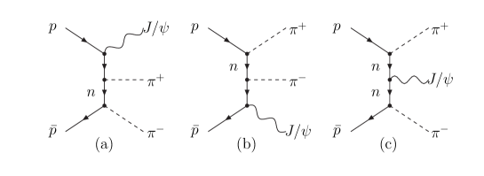
Figure 1: The production of $J/\psi\pi^{+}\pi^{-}$ through the $p\bar{p}$-annihilation

In Fig.1 $n$ denotes the internal neutron line. Again we use effective couplings to calculate the process. We use $-\sqrt{2}g_{pp\pi}\gamma_{5}$ for the $np\pi$ effective vertex, $-g_{pp\pi}\gamma_{5}$ for the $pp\pi$ effective vertex, $ig_{p\bar{p}\psi}\gamma_{\mu}$ for the $J/\psi p\bar{p}$, and $ig_{n\bar{n}\psi}\gamma_{\mu}$ for the $J/\psi n\bar{n}$, respectively. The amplitude from Fig.1 can be expressed as

$$\mathcal{M}_{a} = i2g_{pp\pi}^{2}g_{p\bar{p}\psi}\bar{v}_{\bar{p}\bar{s}}\gamma_{5}\frac{1}{(\not{p}_{-}-\not{\bar{p}})-m_{n}}\gamma_{5}\frac{1}{(\not{p}-\not{p}_{\psi})-m_{p}}\gamma_{\mu}u_{ps}\epsilon_{\psi}^{\ast\mu},$$

$$\mathcal{M}_{b} = i2g_{pp\pi}^{2}g_{p\bar{p}\psi}\bar{v}_{\bar{p}\bar{s}}\gamma_{\mu}\frac{1}{(\not{p}_{\psi}-\not{\bar{p}})-m_{p}}\gamma_{5}\frac{1}{(\not{p}-\not{p}_{+})-m_{n}}\gamma_{5}u_{ps}\epsilon_{\psi}^{\ast\mu},$$

$$\mathcal{M}_{c} = i2g_{pp\pi}^{2}g_{n\bar{n}\psi}\bar{v}_{\bar{p}\bar{s}}\gamma_{5}\frac{1}{(\not{p}_{-}-\not{\bar{p}})-m_{n}}\gamma_{\mu}\frac{1}{(\not{p}-\not{p}_{+})-m_{n}}\gamma_{5}u_{ps}\epsilon_{\psi}^{\ast\mu},$$ (13)

then the total amplitude is the sum:

$$\mathcal{M}[p\bar{p}\to J/\psi\pi^{+}\pi^{-}]=\mathcal{M}[p\bar{p}\rightarrow X\to J/\psi\pi^{+}\pi^{-}]+\mathcal{M}_{a}+\mathcal{M}_{b}+\mathcal{M}_{c}.$$ (14)

The effective coupling $g_{pp\pi}$ is $g_{pp\pi}=13.5$. By using isospin symmetry we have $g_{p\bar{p}\psi}=g_{n\bar{n}\psi}$ and $m_{n}=m_{p}$. The effective coupling $g_{p\bar{p}\psi}$ can be determined from the decay $J/\psi\to p\bar{p}$. It should be noted that for the decay it is possible that another coupling, i.e., the Pauli’s coupling can be appear[18]. We neglect this coupling and get $g_{p\bar{p}\psi}=1.62\times 10^{-3}$ [18]. Although the coupling constants are estimated, but their relative phase is unknown. There are two possible cases: Case 1: The product $g_{p\bar{p}\psi}g_{pp\pi}^{2}$ has the same sign as that of the product $g_{p\bar{p}X}G_{X\psi\rho}G_{\rho\pi\pi}$. Case 2: The two products have different sign. The expression of the amplitude squared is too length because it is a $2\to 3$ body process and we do not try to produce an analytical expression for the total cross section. Instead giving the analytical expression we simply take the amplitude squared to perform the phase space integral numerically. In Fig.2 and Fig.3 we plot the total cross section as functions of the invariant mass $s$ of the $p\bar{p}$ pair, where we take $\Gamma_{X}=2.3$ MeV and the coupling constants estimated before. Fig.2 is for $X(3872)$ as a loosely bound state of $D$-mesons, Fig.3 is for $X(3872)$ as $\chi_{c1}(2P)$.

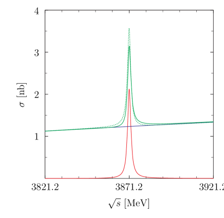
Figure 2: The total cross-section as a function of $\sqrt{s}$ for $X(3872)$ as a loosely bound state of $D$-mesons. The lower resonance curve is without the background, the upper curves are with the back ground. The solid one is for Case 2, while the dashed one is for Case 1.

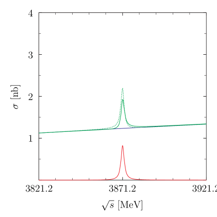
Figure 3: The total cross-section as a function of $\sqrt{s}$ for $X(3872)$ as $\chi_{c1}(2P)$. The lower resonance curve is without the background, the upper curves are with the back ground. The solid one is for Case 2, while the dashed one is for Case 1.

From these figures we clearly see that from the line shape of the cross-section two interpretations of $X(3872)$ can be distinguished. The difference comes from the decay into $J/\psi\pi^{+}\pi^{-}$ with the different assignment of $X(3872)$. We also see that the background is an significant contribution for the production. For the assignment with the bound state of $D$-mesons we have the total cross-section at $\sqrt{s}=3.872$GeV by taking $E_{X}=0.6$ MeV, $\Gamma_{X}=136{\rm keV}\sim 2.3{\rm MeV}$:

$$\sigma[p\bar{p}\rightarrow X\to J/\psi\pi^{+}\pi^{-}]=3.57\sim 443{\rm nb},$$ (15)

for the assignment with $\chi_{c1}(2P)$ we have with $\Gamma_{X}=136{\rm keV}\sim 2.3{\rm MeV}$:

$$\sigma[p\bar{p}\rightarrow X\to J/\psi\pi^{+}\pi^{-}]=2.19\sim 238{\rm nb}.$$ (16)

The main uncertainties in the above come from the unknown width $\Gamma_{X}$. In Fig.4 we plot the dependence of the cross section with different assignments as a function of $\Gamma_{X}$. From Fig.4 we see that there is a strong dependence of the total cross section on the total width and the cross-section with two interpretations are different. Hence the measurement of the cross section will give a clear evidence to indicate which interpretation is the correct one.

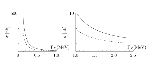
Figure 4: The total cross-section as a function of $\Gamma_{X}$ at the threshold. The solid line is for the interpretation with the $D$-meson bound state, the dashed line is for the interpretation of $\chi_{c1}(2P)$. The curves are for Case 1. The curves for Case 2. are similar.

The luminosity of PANDA can be up to $2\times 10^{32}{\rm cm}^{-2}{\rm s}^{-1}$  [16]. Assuming $50\%$ overall efficiency and 6 months/year data taking, the integrated luminosity is to be $1.5{\rm fb}^{-1}$ per year. With the integrated luminosity and the cross-section obtained here, one can expect $10^{6}\sim 10^{8}$ events per year for the production of $J/\psi\pi^{+}\pi^{-}$ near the threshold. With the large number of events one can study $X(3872)$ in more detail.

With the estimated couplings we can also study the production of $X(3872)$ associated with $\pi^{0}$, i.e., the production away from the resonance region. There are two diagrams for the process given in Fig.5. The calculation of the total cross section is straightforward. The analytical expression for the differential cross-section can be found in [18]. We only give our numerical result here. With the same parameters we obtain the total cross section as a function of $\sqrt{s}$ up to $5$GeV given in Fig.6. From Fig.6 we find that the total cross section of $p\bar{p}\to X\pi^{0}$ is at order of $\sim 100$pb. With the designed luminosity and by considering the branching ratio of decays of $X$ it is likely that such a process can not be observed.

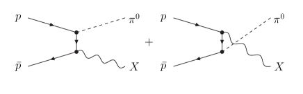
Figure 5: The diagrams for $p\bar{p}\to X\pi^{0}$.

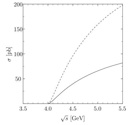
Figure 6: The $s$-dependence of the total cross section of $p\bar{p}\to X\pi^{0}$.

To summarize: In this work we have studied the $X(3872)$-production at PANDA, where two possible interpretations of $X(3872)$ have been assumed. We have found that there will be a large number of events for the process $p\bar{p}\to J/\psi\pi^{+}\pi^{-}$ at the threshold where large fraction of events will be produced from the decay of $X(3872)$. By measuring the cross-section and its $s$-dependence near the threshold one can distinguish the two interpretations. For other possible interpretations like a diquark anti-diquark bound state, a hybrid charmonium state and a tetraquark state, the coupling with $p\bar{p}$ is so far unknown. Once the coupling is estimated, the production rate can be obtained from our results here. If the coupling is not extremely small in comparison with those given in Eq.(3,5), one may still expect that $X(3872)$ can be produced with a not small event number. Hence the study of the $X(3872)$-production at PANDA will provide important information about the structure of $X(3872)$. We have also studied the production associated with $\pi^{0}$. But the cross-section by considering the branching ratio of $X(3872)$ may be too small to be measured.

Acknowledgement:

We would like to thank Prof. H.Q. Zheng, Dr. C. Meng and Dr. Y.J. Zhang for helpful discussions. This work is supported by National Nature Science Foundation of P.R. China.

References

• [1] S. K. Choi et al., Belle Collabloration, Phys. Rev. Lett. 91, 262001 (2003).
• [2] B. Aubert et al., BaBar Collaboration, Phys. Rev. D71, 071103 (2005)
• [3] D. Acosta et al., CDF \@slowromancapii@ Collaboration, Phys. Rev. Lett. 93, 072001 (2004).
• [4] V. M. Abazov et al., D0 Collaboration, Phys. Rev. Lett. 93, 162002 (2004).
• [5] Review of Particle Physics, W. M. Yao et al., J. Phys. G33, 1(2006).
• [6] K. Abe et al., Belle Collaboration, hep-ex/0505038.
• [7] A. Abulencia et al., CDF Collaboration, Phys. Rev. Lett.98, 132002 (2007).
• [8] N. A. Tornqvst, Phys. Lett. B590, 209 (2004), M. B. Voloshin, Phys. Lett. B579, 316 (2004), C. Y. Wong, Phys. Rev. C69, 055202 (2004), E. Braaten and M. Kusunoki, Phys. Rev. D69, 074005 (2004), E. S. Swanson, Phys. Lett. B588, 189 (2004), E. Braaten, et al., Phys. Rev. Lett 93, 162001 (2004), E. S. Swanson, Phys. Lett. B598, 197 (2004), M. B. Voloshin, Phys. Lett. B604, 69 (2004), E. Braaten and M. Kusunoki, Phys. Rev. D71, 074005 (2005).
• [9] C. Meng and K. T. Chao, Phys. Rev. D75, 114002 (2007).
• [10] P. Colangelo, et al., Phys. Lett. B650, 166 (2007).
• [11] J.L. Rosner, Phys. Rev. D74 076006 (2006).
• [12] D.V. Bugg, Phys. Lett. B598 8 (2004)
• [13] L. Maiani, F. Piccinini, A.D. Polosa and V. Riquer, Phys. Rev. D71 014028 (2005).
• [14] B.A. Li, Phys. Lett. B605 306 (2005)
• [15] T.W. Chiu et al., Phys. Lett. B646 95 (2007), Phys. Rev. D73 111503 (2006), D. Ebert, R.N. Faustov and V.O. Galkin, Phys. Lett. B634 214 (2006), R.D. Matheus et al., Phys. Rev. D75 014005 (2007), H. Hogaasen, J.M. Richard and P. Sorba, Phys. Rev. D73 054013 (2006), N. Barnea, J. Vijande and A. Valcarce, Phys. Rev. D73 054004 (2006), Y. Cui et al., High Energy Phys. Nucl. Phys. 31 7 (2007).
• [16] K. T. Brinkmann, Nucl. Instr. and Meth. A549, 146 (2005), P. Hawranek, Int. J. Mod. Phys. A22, 574 (2007).
• [17] E. J. Eichten and C. Quigg, Phys. Rev. D52, 1726 (1995).
• [18] T. Barnes and X. Li, Phys. Rev. D 75, 054018 (2007), T. Barnes, X. Li and W. Roberts, JLAB-THY-07-730, e-Print: arXiv:0709.4491.
• [19] E. Braaten, hep-ph/07111854.
• [20] E. Braaten and M. Kusunoki, Phys. Rev. D 72, 054022 (2005).