Determining the Dark Matter Relic Density in the Minimal Supergravity Stau-Neutralino Coannihilation Region at the Large Hadron Collider

Abstract

We examine the stau-neutralino coannihilation (CA) mechanism of the early universe. We use the minimal supergravity (mSUGRA) model and show that from measurements at the Large Hadron Collider one can predict the dark matter relic density with an uncertainty of 6% with 30 ${\rm fb}^{-1}$ of data, which is comparable to the direct measurement by Wilkinson Microwave Anisotropy Probe. This is done by measuring four mSUGRA parameters $m_{0}$, $m_{1/2}$, $A_{0}$ and $\tan\beta$ without requiring direct measurements of the top squark and bottom squark masses. We also provide precision measurements of the gaugino, squark, and lighter stau masses in this CA region without assuming gaugino universality.

One of the important aspects of supersymmetry (SUSY), particularly when it is combined with supergravity grand unification (SUGRA GUT) sugra1 ; sugra2 , is that it resolves a number of the problems inherent in the standard model (SM). Aside from solving the gauge hierarchy problem and predicting grand unification at the GUT scale $M_{\rm G}\sim 10^{16}$ GeV, subsequently verified at LEP LEP , SUGRA GUT allows for the spontaneous breaking of SUGRA at the $M_{\rm G}$ scale in a hidden sector, leading to an array of soft breaking masses. The renormalization group equations then show that this breaking of SUGRA leads naturally to the breaking of $SU(2)\times U(1)$ of the SM at the electroweak scale, with SUSY breaking masses around a TeV for most of the SUSY parameter space.

An additional feature of SUSY is that models with $R$-parity invariance give rise to a cold dark matter (CDM) candidate gw , which is generally the lightest neutralino ($\tilde{\chi}_{1}^{0}$). The CERN Large Hadron Collider (LHC) should be able to produce the $\tilde{\chi}_{1}^{0}$, and study its properties. Direct detection experiments for Milky Way DM would allow for a determination of the DM mass and its nuclear cross section. If these are in agreement with the LHC determination of the $\tilde{\chi}_{1}^{0}$ properties, it would help confirm the important point that the Milky Way DM was indeed the $\tilde{\chi}_{1}^{0}$. However, this would not explicitly verify that the $\tilde{\chi}_{1}^{0}$ was the DM relic particle produced during the Big Bang. To do this, one would need to deduce the relic density $\Omega_{\mbox{$\tilde{\chi}_{1}^{0}$}}h^{2}$ and compare with $\Omega_{\rm CDM}h^{2}$ as measured astronomically by Wilkinson Microwave Anisotropy Probe (WMAP) WMAP .

In this Letter we describe a series of measurements in the stau-neutralino ($\tilde{\tau}_{1}$-$\tilde{\chi}_{1}^{0}$) coannihilation (CA) region where, in the early universe, the $\tilde{\tau}_{1}$ and the $\tilde{\chi}_{1}^{0}$ annihilate together into SM particles, determining the relic DM abundance observed today. We show how to measure the sparticle masses, confirm we are in the CA region, measure the SUSY parameters, and establish a prediction of $\Omega_{\mbox{$\tilde{\chi}_{1}^{0}$}}h^{2}$.

To carry out this analysis it is necessary to assume a model that encompasses both LHC phenomena and early universe physics. Since the analysis is new and quite complicated we consider the simplest SUGRA model (minimal SUGRA or mSUGRA) sugra1 with universal soft breaking masses. However, we show below that it is possible to test experimentally gaugino universality; other non-universality models will be considered elsewhere. The mSUGRA model depends on one sign and four parameters: $m_{0}$ (universal sfermion mass), $m_{1/2}$ (universal gaugino mass), $A_{0}$ (universal soft breaking trilinear coupling constant), $\tan\beta$ (the ratio of vacuum expectation values of two Higgs doublets), and the sign of $\mu$ (the bilinear Higgs coupling constant). After we include all experimental constraints LEP , the allowed mSUGRA parameter space with $\mu>0$ (as preferred by $b\rightarrow s\gamma$ and the muon $g-2$ BNLg-2 ) has three distinct regions picked out by the CDM constraints darkrv : (i) the CA region where both $m_{0}$ and $m_{1/2}$ can be small, (ii) the focus-point region where the $\tilde{\chi}_{1}^{0}$ has a large Higgsino component and $m_{0}$ is very large but $m_{1/2}$ is small, and (iii) the funnel region where both $m_{0}$ and $m_{1/2}$ are large and the neutralinos can annihilate through heavy Higgs bosons ($2M_{\mbox{$\tilde{\chi}_{1}^{0}$}}\simeq M_{A_{0},H_{0}}$). We consider here the CA region with $\mu>0$. This region is generic for a wide class of SUGRA GUT models (with or without gaugino universality). If the muon $g-2$ anomaly maintains, then the focus-point and funnel regions are essentially eliminated.

The CA region has a striking characteristic of the $\tilde{\tau}_{1}$ and $\tilde{\chi}_{1}^{0}$ being nearly degenerate $i.e.$, $\mbox{$\Delta M$}\equiv M_{\mbox{$\tilde{\tau}_{1}$}}-M_{\mbox{$\tilde{\chi}_{1}^{0}$}}\sim$ (5-15) GeV. Thus, the $\mbox{$\tilde{\chi}_{2}^{0}$}\rightarrow\tau\mbox{$\tilde{\tau}_{1}$}\rightarrow\tau\tau\mbox{$\tilde{\chi}_{1}^{0}$}$ decays are dominant and the branching ratio for $\mbox{$\tilde{\chi}_{2}^{0}$}\rightarrow\ell\mbox{$\tilde{\ell}_{R}$}\rightarrow\ell\ell\mbox{$\tilde{\chi}_{1}^{0}$}$ is essentially zero ($\ell$= $e$ or $\mu$, and $\tilde{\ell}_{R}$ is the lighter selectron or smuon). The existence of this near degeneracy would be a strong indication that we are in the CA region.

In order to determine $\Omega_{\mbox{$\tilde{\chi}_{1}^{0}$}}h^{2}$ one must know all the mSUGRA parameters. In a previous study polsello , $m_{1/2}$, $m_{0}$, $A_{0}$, and $\tan\beta$ were determined in the bulk region assuming that it is possible to measure the gluino ($\tilde{g}$), squark ($\tilde{q}$), lighter bottom squark (sbottom or $\tilde{b}_{1}$), $\tilde{\ell}_{R}$, $\tilde{\chi}_{2}^{0}$, and $\tilde{\chi}_{1}^{0}$ masses in $\mbox{$\tilde{g}$}\rightarrow b\mbox{$\tilde{b}_{1}$}$ and $\mbox{$\tilde{q}_{L}$}\rightarrow q\mbox{$\tilde{\chi}_{2}^{0}$}\rightarrow q\ell\mbox{$\tilde{\ell}_{R}$}\rightarrow q\ell\ell\mbox{$\tilde{\chi}_{1}^{0}$}$ decays, using “end-point” techniques hinch1 . The determination of $M_{\tilde{b}_{1}}$ is very difficult if both $\mbox{$\tilde{g}$}\rightarrow t\mbox{$\tilde{t}_{1}$}$ (here $\tilde{t}_{1}$ is the lighter top squark or stop) and $\mbox{$\tilde{g}$}\rightarrow b\mbox{$\tilde{b}_{1}$}$ can occur gmo and the methodology of disentangling this background is not known yet. Also these techniques cannot be utilized for the CA case because the $\mbox{$\tilde{\chi}_{2}^{0}$}\rightarrow\ell\mbox{$\tilde{\ell}_{R}$}\rightarrow\ell\ell\mbox{$\tilde{\chi}_{1}^{0}$}$ decay is essentially absent.

While the CA region is particularly challenging, we show that it is indeed possible to determine all four parameters accurately from measurements at the LHC. It has been recently shown LHCtwotau ; LHCthreetau that the CA region can be established and that a measurement of $\Delta M$ can be made (provided the $\tau$ identification can be done for visible $\tau$ $\mbox{$p_{\rm T}^{\rm vis}$}>20\ \mbox{${\rm GeV}$}$) assuming $A_{0}$ and $\tan\beta$ are known. The small $\Delta M$ value is experimentally characterized by a low energy $\tau$ from a $\mbox{$\tilde{\tau}_{1}$}\rightarrow\tau\mbox{$\tilde{\chi}_{1}^{0}$}$ decay. With the addition of some new datasets and variables, in particular with final state $b$-quark jets, we show that we can (a) measure the $\tilde{g}$, $\tilde{q}_{L}$, $\tilde{\chi}_{2}^{0}$, $\tilde{\chi}_{1}^{0}$, and $\tilde{\tau}_{1}$ masses in the case of $M_{\mbox{$\tilde{q}$}}\simeq M_{\mbox{$\tilde{g}$}}\gg M_{\mbox{$\tilde{\chi}_{2}^{0}$},\mbox{$\tilde{\chi}_{1}^{\pm}$}}$ without the mSUGRA assumption, (b) determine the mSUGRA parameters, and (c) predict $\Omega_{\mbox{$\tilde{\chi}_{1}^{0}$}}h^{2}$, which can be compared with the astronomical determination of $\Omega_{\rm CDM}h^{2}$. Of particular note, our method effectively obviates the need to separate the final states arising from the third generation sparticles, such as stops ($\tilde{t}_{1}$, $\tilde{t}_{2}$), sbottoms ($\tilde{b}_{1}$, $\tilde{b}_{2}$), and staus ($\tilde{\tau}_{1}$, $\tilde{\tau}_{2}$). The procedure of extracting the model parameters is general and can be applied to other regions of the parameter space or to more general SUGRA models.

We select an mSUGRA reference point, shown in Table 1, where $\Omega_{\mbox{$\tilde{\chi}_{1}^{0}$}}h^{2}$ = 0.10 and $\Delta M$ = 10.6 GeV. The total production cross section at the LHC is 9.1 pb where the $\tilde{g}$$\tilde{q}$ production has the largest contribution. Events are generated using ISAJET isajet , followed by the PGS4 detector simulation pgs . We analyze three samples with the final state of large transverse missing energy (${E\!\!\!\!/_{\rm T}}$) along with jets ($j$’s), $\tau$’s, and $b$’s: (i) 2$\tau$ + 2$j$ + ${E\!\!\!\!/_{\rm T}}$, (ii) 4$j$ + ${E\!\!\!\!/_{\rm T}}$, and (iii) 1$b$ + 3$j$ + ${E\!\!\!\!/_{\rm T}}$. The kinematics in both 2$\tau$ + 2$j$ + ${E\!\!\!\!/_{\rm T}}$ and the 1$b$ + 3$j$ + ${E\!\!\!\!/_{\rm T}}$ samples depend on all four mSUGRA parameters, while the 4$j$ + ${E\!\!\!\!/_{\rm T}}$ sample is mostly sensitive to $m_{0}$ and $m_{1/2}$.

Table 1: SUSY reference point (masses in GeV) $m_{1/2}$ = 350 GeV, $m_{0}$ = 210 GeV, $\tan\beta=40$, $\mbox{$A_{0}$}=0$, and $\mu>0$.

$\tilde{g}$	$\begin{array}[]{c}\mbox{$\tilde{u}_{L}$}\\ \mbox{$\tilde{u}_{R}$}\end{array}$	$\begin{array}[]{c}\mbox{$\tilde{t}_{2}$}\\ \mbox{$\tilde{t}_{1}$}\end{array}$	$\begin{array}[]{c}\mbox{$\tilde{b}_{2}$}\\ \mbox{$\tilde{b}_{1}$}\end{array}$	$\begin{array}[]{c}\mbox{$\tilde{e}_{L}$}\\ \mbox{$\tilde{e}_{R}$}\end{array}$	$\begin{array}[]{c}\mbox{$\tilde{\tau}_{2}$}\\ \mbox{$\tilde{\tau}_{1}$}\end{array}$	$\begin{array}[]{c}\mbox{$\tilde{\chi}_{2}^{0}$}\\ \mbox{$\tilde{\chi}_{1}^{0}$}\end{array}$	$\Delta M$	$\begin{array}[]{c}M_{\mbox{$\tilde{g}$}}/M_{\mbox{$\tilde{\chi}_{1}^{0}$}}\\ M_{\mbox{$\tilde{g}$}}/M_{\mbox{$\tilde{\chi}_{2}^{0}$}}\end{array}$
831	$\begin{array}[]{c}748\\ 725\end{array}$	$\begin{array}[]{c}728\\ 561\end{array}$	$\begin{array}[]{c}705\\ 645\end{array}$	$\begin{array}[]{c}319\\ 251\end{array}$	$\begin{array}[]{c}329\\ 151.3\end{array}$	$\begin{array}[]{c}260.3\\ 140.7\end{array}$	10.6	$\begin{array}[]{c}5.91\\ 3.19\end{array}$

The primary SM backgrounds for the 2$\tau$ + 2$j$ + ${E\!\!\!\!/_{\rm T}}$ final state (and the other two samples) are from $t\bar{t}$, $W$+jets, $Z$+jets and QCD production. The sample is selected using the following cuts LHCtwotau : (a) $N_{\tau}\geq 2$ ($|\eta|<2.5$, $\mbox{$p_{\rm T}^{\rm vis}$}>20\ \mbox{${\rm GeV}$}$, but $>40\ \mbox{${\rm GeV}$}$ for the leading $\tau$); (b) $N_{j}\geq 2$ ($|\eta|<2.5$, $\mbox{$E_{\rm T}$}>100\ \mbox{${\rm GeV}$}$); (c) $\mbox{${E\!\!\!\!/_{\rm T}}$}>180\ \mbox{${\rm GeV}$}$ and $\mbox{$E_{\rm T}$}^{j\rm{1}}+\mbox{$E_{\rm T}$}^{j\rm{2}}$ + ${E\!\!\!\!/_{\rm T}}$ $>$ 600 GeV; and (d) veto the event if any of the two leading jets are identified as a $b$ jet. In order to identify $\mbox{$\tilde{\chi}_{2}^{0}$}\rightarrow\tau\mbox{$\tilde{\tau}_{1}$}\rightarrow\tau\tau\mbox{$\tilde{\chi}_{1}^{0}$}$ decays we categorize all pairs of $\tau$’s into opposite-sign (OS) and like-sign (LS) combinations, and then use the OS minus LS (OS$-$LS) distributions to effectively reduce the SM events as well as the combinatoric SUSY backgrounds. We reconstruct the decay chains of $\mbox{$\tilde{q}_{L}$}\rightarrow q\mbox{$\tilde{\chi}_{2}^{0}$}\rightarrow q\tau\mbox{$\tilde{\tau}_{1}$}\rightarrow q\tau\tau\mbox{$\tilde{\chi}_{1}^{0}$}$ using the following five kinematic variables: (1) $\alpha$, the slope of the $p_{\rm T}^{\rm vis}$ distribution for the lower energy $\tau$ in the OS$-$LS di-$\tau$ pairs, (2) $M_{\tau\tau}^{\rm peak}$, the peak position of the visible di-$\tau$ invariant mass distribution, (3) $M_{j\tau\tau}^{\rm peak}$, the peak position of the invariant $j$-$\tau$-$\tau$ mass distribution, and (4, 5) $M_{j\tau}^{\rm peak}$, the peak position of the invariant $j$-$\tau$ mass distribution where each $\tau$ from the OS$-$LS di-$\tau$ pair is examined separately. Note that we have used the peak positions instead of the end-points because of the $\tau$’s in the final state.

We follow the recommendation of Ref. hinch1 for the 4$j$ + ${E\!\!\!\!/_{\rm T}}$ sample. The peak value, $M_{\rm eff}^{\rm peak}$, of the variable $\mbox{$M_{{\rm eff}}$}\equiv\mbox{${E\!\!\!\!/_{\rm T}}$}\ +\sum_{{\rm 4~{}jets}}\mbox{$E_{\rm T}$}^{j}$, which is a function of only the $\tilde{g}$ and $\tilde{q}$ masses, is reconstructed for each event that passes the following selection cuts: (a) $N_{j}\geq 4$ ($|\eta|<2.5$, $\mbox{$E_{\rm T}$}>50\ \mbox{${\rm GeV}$}$, but $>100\ \mbox{${\rm GeV}$}$ for the leading jet); (b) $\mbox{${E\!\!\!\!/_{\rm T}}$}>100\ \mbox{${\rm GeV}$}$; (c) Transverse sphericity $>$ 0.2; (d) Veto on all events containing an isolated electron or muon with $\mbox{$p_{\rm T}$}>15\ \mbox{${\rm GeV}$}$ and $|\eta|<2.5$; and (e) $\mbox{${E\!\!\!\!/_{\rm T}}$}>0.2\mbox{$M_{{\rm eff}}$}$. Again we require that none of these jets be identified as a $b$ jet.

Similar cuts are used to make the 1$b$ + 3$j$ + ${E\!\!\!\!/_{\rm T}}$ sample. We introduce a new variable, $M_{{\rm eff}}^{(b)\rm peak}$, similar to $M_{{\rm eff}}^{\rm peak}$, but requiring that the leading jet be from a $b$ quark.

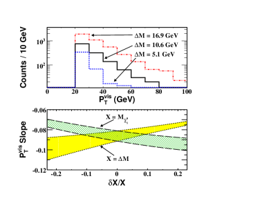
Figure 1: [top] The $p_{\rm T}^{\rm vis}$ distribution of the lower-energy $\tau$’s using the OS$-$LS technique in the three samples (arbitrary luminosity) of SUSY events with $\Delta M$ = 5.1, 10.6 and 16.9 GeV, where only the $\tilde{\tau}_{1}$ mass is changed at our reference point. [bottom] The $p_{\rm T}^{\rm vis}$ slope (as $\alpha$ in the text) as a function of the relative change of $M_{\tilde{\tau}_{1}}$ (therefore $\Delta M$) or $M_{\mbox{$\tilde{\chi}_{1}^{0}$}}$ from its reference value with the other SUSY masses fixed. The bands correspond to statistical uncertainties with 10 ${\rm fb}^{-1}$.

The measurement of a small value of $\alpha$ from the 2$\tau$ + 2$j$ + ${E\!\!\!\!/_{\rm T}}$ sample indicates low energy $\tau$’s in the final state (thus $\Delta M$ is small) and provides a smoking-gun signal for the CA region. In Fig. 1, we show the $p_{\rm T}^{\rm vis}$ distributions obtained by the OS$-$LS technique for various $\Delta M$ values. Note that $\alpha$ only depends on $M_{\mbox{$\tilde{\tau}_{1}$}}$ and $M_{\mbox{$\tilde{\chi}_{1}^{0}$}}$ (see Fig. 1).

To get a set of measurements of the sparticle masses we use the remaining variables from the 2$\tau$ + 2$j$ + ${E\!\!\!\!/_{\rm T}}$ and 4$j$ + ${E\!\!\!\!/_{\rm T}}$ samples. The variables $M_{j\tau\tau}^{\rm peak}$ and $M_{j\tau}^{\rm peak}$ probe the $\mbox{$\tilde{q}_{L}$}\rightarrow q\mbox{$\tilde{\chi}_{2}^{0}$}\rightarrow q\tau\mbox{$\tilde{\tau}_{1}$}\rightarrow q\tau\tau\mbox{$\tilde{\chi}_{1}^{0}$}$ decay chains. To help identify these chains we additionally require OS$-$LS di-$\tau$ pairs with $M_{\tau\tau}<M_{\tau\tau}^{\mbox{\rm end-point}}$ and construct $M_{j\tau\tau}$ for every jet with $\mbox{$E_{\rm T}$}>100\ \mbox{${\rm GeV}$}$ in the event. With three jets, there are three masses: $M_{j\tau\tau}^{(1)}$, $M_{j\tau\tau}^{(2)}$, and $M_{j\tau\tau}^{(3)}$, in decreasing order. We choose $M_{j\tau\tau}^{(2)}$ for this analysis hinch1 . Figure 2 shows the $M_{j\tau\tau}^{(2)}$ distributions for two different $\tilde{q}_{L}$ masses, and $M_{j\tau\tau}^{(2)\rm peak}$ as a function of $M_{\mbox{$\tilde{q}_{L}$}}$ and $M_{\mbox{$\tilde{\chi}_{1}^{0}$}}$, keeping $\Delta M$ constant. Similarly, one can show that the $M_{j\tau}^{(2)\rm peak}$ value depends on the $\tilde{q}_{L}$, $\tilde{\chi}_{2}^{0}$, $\tilde{\tau}_{1}$  and $\tilde{\chi}_{1}^{0}$  masses. The value of $M_{{\rm eff}}^{\rm peak}$, extracted from 4$j$ + ${E\!\!\!\!/_{\rm T}}$ sample, has been shown to be a function of only the $\tilde{q}_{L}$ and $\tilde{g}$ masses.

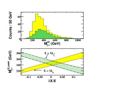
Figure 2: [top] The $M_{j\tau\tau}^{(2)}$ distributions using the OS$-$LS technique for SUSY events at our reference point, but with $M_{\mbox{$\tilde{q}_{L}$}}$ = 660 GeV (yellow or light gray histogram) and 840 GeV (green or dark gray histogram), where 748 GeV is our reference point; [bottom] The peak position of the mass distribution as a function of $M_{\mbox{$\tilde{\chi}_{1}^{0}$}}$ or $M_{\mbox{$\tilde{q}_{L}$}}$. The bands correspond to statistical uncertainties with 10 ${\rm fb}^{-1}$.

The determination of the sparticle masses is done by inverting the six functional relationships between the variables and the sparticle masses to simultaneously solve for the $\tilde{g}$, $\tilde{\chi}^{0}_{1,2}$, $\tilde{\tau}_{1}$, and average $\tilde{q}_{L}$ masses and their uncertainties. The six parametrized functions are: $M_{\tau\tau}^{\rm peak}$ = $f_{1}$($M_{\mbox{$\tilde{\chi}_{2}^{0}$}}$, $M_{\mbox{$\tilde{\chi}_{1}^{0}$}}$, $\Delta M$), $\alpha$ = $f_{2}$($M_{\mbox{$\tilde{\chi}_{1}^{0}$}}$, $\Delta M$), $M_{j\tau\tau}^{(2)\rm peak}$ = $f_{3}$($M_{\mbox{$\tilde{q}_{L}$}}$, $M_{\mbox{$\tilde{\chi}_{2}^{0}$}}$, $M_{\mbox{$\tilde{\chi}_{1}^{0}$}}$), $M_{j\tau(1,2)}^{(2)\rm peak}$ = $f_{4,5}$($M_{\mbox{$\tilde{q}_{L}$}}$, $M_{\mbox{$\tilde{\chi}_{2}^{0}$}}$, $M_{\mbox{$\tilde{\chi}_{1}^{0}$}}$, $\Delta M$), and $M_{{\rm eff}}^{\rm peak}$ = $f_{6}$($M_{\mbox{$\tilde{q}_{L}$}}$, $M_{\mbox{$\tilde{g}$}}$). With 10 ${\rm fb}^{-1}$ of data, we obtain (in GeV) $M_{\mbox{$\tilde{g}$}}=831\pm 28$, $M_{\mbox{$\tilde{\chi}_{2}^{0}$}}=260\pm 15$, $M_{\mbox{$\tilde{\chi}_{1}^{0}$}}=141\pm 19$, $\mbox{$\Delta M$}=10.6\pm 2.0$, and $M_{\mbox{$\tilde{q}_{L}$}}=748\pm 25$ uncertainties . The accurate determination of $\Delta M$ would also confirm that we are in the CA region. We also test the universality of the gaugino masses at the GUT scale. We measure $M_{\mbox{$\tilde{g}$}}/M_{\mbox{$\tilde{\chi}_{1}^{0}$}}=5.9\pm 0.8$ and $M_{\mbox{$\tilde{g}$}}/M_{\mbox{$\tilde{\chi}_{2}^{0}$}}=3.1\pm 0.2$, validating the universality relations to $14\%$ and $6\%$, repectively. This non-trivial determination of the additional gaugino masses along with the mSUGRA parameters require all six observables. The formalism developed here can work for other model with similar two-body decay processes.

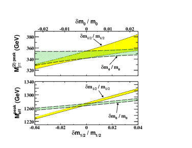
Figure 3: The dependence of $M_{j\tau\tau}^{(2)\rm peak}$ (top) and $M_{{\rm eff}}^{\rm peak}$ (bottom) as a function of $m_{1/2}$ and $m_{0}$. The bands correspond to statistical uncertainties with 10 ${\rm fb}^{-1}$.

Since our primary goal is to determine $\Omega_{\mbox{$\tilde{\chi}_{1}^{0}$}}h^{2}$ in the mSUGRA model we next determine $m_{0}$, $m_{1/2}$, $A_{0}$ and $\tan\beta$. $M_{\rm eff}^{\rm peak}$ and $M_{j\tau\tau}^{(2)\rm peak}$ are insensitive to $A_{0}$ and $\tan\beta$, and provide a direct handle on $m_{0}$ and $m_{1/2}$ because they depend only on the $\tilde{q}_{L}$ (first two generations), $\tilde{g}$, $\tilde{\chi}_{2}^{0}$ and $\tilde{\chi}_{1}^{0}$ masses (see Fig. 3). On the other hand, $M_{\tau\tau}^{\rm peak}$ and $M_{{\rm eff}}^{(b)\rm peak}$  provide a direct handle on $A_{0}$ and $\tan\beta$. $M_{\tau\tau}^{\rm peak}$ depends on $M_{\tilde{\tau}_{1}}$; $M_{{\rm eff}}^{(b)\rm peak}$ depends on $M_{\tilde{t}_{1}}$ and $M_{\tilde{b}_{1}}$, since both the $\tilde{t}_{1}$ and $\tilde{b}_{1}$ decays always produce at least one $b$ jet in the final state. Figure 4 shows the values of $M_{\tau\tau}^{\rm peak}$ and $M_{{\rm eff}}^{(b)\rm peak}$ as functions of $A_{0}$ and $\tan\beta$ since the off-diagonal elements of $\tilde{t}_{1}$ and $\tilde{b}_{1}$/$\tilde{\tau}_{1}$ mass matrices depend on $M_{t}(A_{t}+\mu\cot\beta)$ and $M_{b/\tau}(A_{b/\tau}+\mu\tan\beta)$, respectively. Combining these four measurements and inverting, we find $m_{0}=210\pm 4\ \mbox{${\rm GeV}$}$, $m_{1/2}=350\pm 4\ \mbox{${\rm GeV}$}$, $A_{0}=0\pm 16\ \mbox{${\rm GeV}$}$, and $\tan\beta=40\pm 1$ with 10 ${\rm fb}^{-1}$ of data uncertainties .

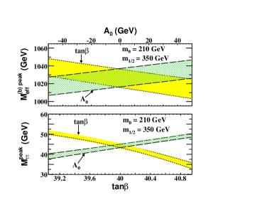
Figure 4: The dependence of $M_{{\rm eff}}^{(b)\rm peak}$ (top) and $M_{\tau\tau}^{\rm peak}$ (bottom) as a function of $\tan\beta$ and $A_{0}$. The bands correspond to statistical uncertainties with 10 ${\rm fb}^{-1}$.

After measuring the mSUGRA variables we calculate $\Omega_{\mbox{$\tilde{\chi}_{1}^{0}$}}h^{2}$ using DARKSUSY darksusy . The calculation also involves the $\tilde{\chi}_{1}^{0}$ mixing matrix which we have determined in the mSUGRA case. In the CA region, $\Omega_{\mbox{$\tilde{\chi}_{1}^{0}$}}h^{2}$ depends crucially on $\Delta M$ due to the Boltzmann suppression factor $e^{-\Delta M/k_{B}T}$ in the relic density formula gs . Figure 5 shows contour plots of the 1$\sigma$ uncertainty in the $\Omega_{\mbox{$\tilde{\chi}_{1}^{0}$}}h^{2}$-$\Delta M$ plane. The uncertainty on $\Omega_{\mbox{$\tilde{\chi}_{1}^{0}$}}h^{2}$ is 11 (4.8)% at 10 (50) ${\rm fb}^{-1}$ uncertainties . Note that it is 6.2% at 30 ${\rm fb}^{-1}$ rel , comparable to that of the WMAP measurement WMAP .

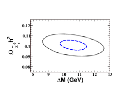
Figure 5: Contour plot of the 1$\sigma$ uncertainty in the $\Omega_{\mbox{$\tilde{\chi}_{1}^{0}$}}h^{2}$-$\Delta M$ plane with 10 and 50 ${\rm fb}^{-1}$ (outer and inner ellipses).

In conclusion, we have established a technique for a precision measurement of $\Omega_{\mbox{$\tilde{\chi}_{1}^{0}$}}h^{2}$ at the LHC in the $\tilde{\tau}_{1}$-$\tilde{\chi}_{1}^{0}$ CA region of the mSUGRA model. This is done using only the model parameters, determined by the kinematical analyses of 3 samples of ${E\!\!\!\!/_{\rm T}}$ + $j$’s (+ $\tau$’s) events with and without $b$ jets. The accuracy of the $\Omega_{\mbox{$\tilde{\chi}_{1}^{0}$}}h^{2}$ calculation at 30 ${\rm fb}^{-1}$ of data is expected to be comparable to that of $\Omega_{\rm CDM}h^{2}$ by WMAP. This approach will allow us to determine the relic abundance at the LHC for any model where the CA is dominant in the early universe. Thus, it is possible to confirm that the DM we observe today were $\tilde{\chi}^{0}_{1}$’s created in the early universe.

We would like to thank F.E. Paige, M.M. Nojiri, G. Polesello, and D.R. Tovey for useful discussions. This work was supported in part by a DOE grant DE-FG02-95ER40917 and NSF grant DMS 0216275. A.G. is supported by DOEd GAANN.

References

(1)
A.H. Chamseddine, R. Arnowitt, and P. Nath, Phys. Rev. Lett. 49, 970 (1982).
(2)
L. Hall, J. Lykken, and S. Weinberg, Phys. Rev. D27, 2359 (1983);
P. Nath, R. Arnowitt, and A.H. Chamseddine, Nucl. Phys. B227, 121 (1983).
For a review, see P. Nilles, Phys. Rep. 100, 1 (1984).
(3)
Particle Data Group, S. Eidelman ,
Phys. Lett. B592, 1 (2004).
(4)
H. Goldberg,
Phys. Rev. Lett. 50, 1419 (1983).
(5)
WMAP Collaboration, D.N. Spergel et al., Astrophys. J. Suppl. 148 (2003) 175.
(6)
Muon Collaboration, G. W. Bennett et al.,
Phys. Rev. Lett. 92, 161802 (2004);
S. Eidelman,
Acta Phys. Polon. B38, 3015 (2007).
(7)
J. Ellis ,
Phys. Lett. B565, 176 (2003);
R. Arnowitt,
B. Dutta, and B. Hu, arXiv:hep-ph/0310103;
H. Baer ,
J. High Energy Phys. 06 (2003) 054;
B. Lahanas and D.V. Nanopoulos, Phys. Lett. B568, 55 (2003);
U. Chattopadhyay, A. Corsetti, and P. Nath,
Phys. Rev. D68, 035005 (2003);
E. Baltz and P. Gondolo, J. High Energy Phys. 10 (2004) 052.
(8)
G. Polesello and D. R. Tovey,
J. High Energy Phys. 05 (2004) 071;
M. M. Nojiri, G. Polesello, and D. R. Tovey,
J. High Energy Phys. 03 (2006) 063.
(9)
I. Hinchliffe ,
Phys. Rev. D55, 5520 (1997);
I. Hinchliffe and F.E. Paige,
Phys. Rev. D61, 095011 (2000).
(10)
B.K. Gjelsten, D.J. Miller, and P. Osland,
J. High Energy Phys. 12 (2004) 003.
(11)
R. Arnowitt ,
Phys. Lett. B639, 46 (2006).
(12)
R. Arnowitt ,
Phys. Lett. B649, 73 (2007).
(13)
F.E. Paige ,
arXiv:hep-ph/0312045.
We use ISAJET version 7.64 with TAUOLA.