Spontaneous R-parity violation: Lightest neutralino decays and neutrino mixing angles at future colliders

Abstract

We study the decays of the lightest supersymmetric particle (LSP) in models with spontaneously broken R-parity. We focus on the two cases that the LSP is either a bino or a neutral singlet lepton. We work out the most important phenomenological differences between these two scenarios and discuss also how they might be distinguished from explicit R-Parity breaking models. In both cases we find that certain ratios of decay branching ratios are correlated with either the solar or the atmospheric (and reactor) neutrino angle. The hypothesis that spontaneous R-Parity violation is the source of the observed neutrino masses is therefore potentially testable at the LHC.

I Introduction

Experiments on solar and atmospheric neutrinos have demonstrated that neutrinos have non-zero masses and mixing angles Fukuda:1998mi ; Ahmad:2002jz ; Eguchi:2002dm . Indeed, with the latest experimental data by the MINOS Collaboration:2007zza and KamLAND KamLAND2007 collaborations neutrino oscillation experiments truly have entered the precision era Maltoni:2004ei .

Many models have been proposed, which potentially can explain these data. Certainly the most popular are variants based on the see-saw mechanism Minkowski:1977sc ; Yanagida:1979as ; Gell-Mann:1980vs ; Mohapatra:1979ia ; Schechter:1980gr . However, the classical seesaw mechanism puts the scale of lepton number violation near the grand unification scale and, therefore, can not be directly tested. Indirect tests of the seesaw might be possible, if low-scale supersymmetry is realized in nature Deppisch:2002vz ; Blair:2002pg ; Freitas:2005et ; Buckley:2006nv ; Deppisch:2007xu . Measurements of masses and branching ratios of supersymmetric particles can be used to obtain indirect information on the range of allowed seesaw parameters, if some specific scenarios for the soft-breaking parameters are assumed Blair:2002pg ; Freitas:2005et ; Buckley:2006nv . On the other hand, a number of neutrino mass models exist, in which neutrino masses are generated at the electro-weak scale. Examples include the Babu-Zee model Babu:1988ki , Leptoquarks AristizabalSierra:2007nf or in case of supersymmetry the breaking of R-parity Hall:1984id . These low energy models usually lead to testable predictions for future colliders. For example, in the case of R-parity violation ($R_{p}/\;\>\hskip 1.99997pt$), in particular for models based on bilinear R-parity breaking terms Hirsch:2004he , correlations between certain branching ratios of the lightest supersymmetric particle decays and the measured neutrino mixing angles have been found Porod:2000hv ; Restrepo:2001me ; Hirsch:2002ys ; Bartl:2003uq ; Hirsch:2003fe .

In $R_{p}/\;\>\hskip 1.99997pt$the neutralino as a dark matter candidate is lost. Recent WMAP data Spergel:2006hy , however, have confirmed the existence of non-baryonic dark matter and measured its contribution to the energy budget of the universe with unprecedented accuracy. Thus, in $R_{p}/\;\>\hskip 1.99997pt$one needs a non-standard explanation of dark matter (DM). Examples for DM candidates in $R_{p}/\;\>\hskip 1.99997pt$include (i) light gravitinos Borgani:1996ag ; Takayama:2000uz ; Hirsch:2005ag , (ii) the axion Kim:1986ax ; Raffelt:1996wa or (iii) its superpartner, the axino Chun:1999cq ; Hirsch:2005jn , to mention a few.

Whether R-parity is conserved or not can, in principle, be easily decided in the case of explicit R-parity violation since (a) neutrino physics implies that the lightest supersymmetric particle (LSP) will decay inside a typical detector of existing and future high energy experiments Porod:2000hv ; Hirsch:2003fe and (b) the branching fraction for (completely) invisible LSP decays is at most ${\cal O}(10\%)$ and typically smallerPorod:2000hv ; Hirsch:2006di . Spontaneous violation of R-parity (s-$R_{p}/\;\>\hskip 1.99997pt$) Aulakh:1982yn ; Masiero:1990uj , on the other hand, implies the existence of a Goldstone boson, the majoron (J). In s-$R_{p}/\;\>\hskip 1.99997pt$the lightest neutralino can then decay according to $\chi^{0}\rightarrow J+\nu$, i.e. completely invisible. It has been shown Hirsch:2006di that this decay mode can in fact be the dominant one, with branching ratios close to 100 %, despite the smallness of neutrino masses, in case the scale of R-parity breaking is relatively low. In this limit, the accelerator phenomenology of models with spontaneous violation of R-parity can resemble the MSSM with conserved R-parity and large statistics might be necessary before it can be established that R-parity indeed is broken.

In this paper we study scenarios where the lightest neutralino is the LSP focusing on two representative examples: (i) a bino-like LSP as this case has been extensively studied in the literature, both in case of conserved R-parity as well as (explicitly) broken R-parity. We will re-iterate our previous result Hirsch:2006di that there are regions in parameter space, where it will be difficult to obtain clarity about the underlying model in the first years of LHC. We will also discuss, how measurements of branching ratios can lead to tests of the model as the origin of the neutrino mass, in case sufficient statistics for the final states with charged leptons can be obtained. (ii) A singlino-like LSP. This case has not been studied in the past but it is the only part of the allowed parameter space where singlinos can be produced and studied at future accelerators. In addition, this case allows interesting cross-checks with respect to neutrino physics different from a bino LSP.

The paper is organized as follows: in Sect. II we present the model with special emphasis on neutrino physics as well as the most important couplings of the lightest neutralino. In Sect. III we discuss production and decays of the lightest neutralino at the LHC as well as a future International Linear Collider (ILC) putting some emphasis on how to distinguish bino and singlino LSPs. In Sect. IV we discuss the different correlations between ratios of neutralino decay branching ratios and neutrino mixing angles. Finally, we draw our conclusions in Sect. V.

II Spontaneous R-parity violation

II.1 Model basics

Spontaneous breaking of a global symmetry leads to a Goldstone boson, in case of lepton number breaking usually called the Majoron. Spontaneous breaking of R-parity through left sneutrinos Aulakh:1982yn , produces a doublet Majoron, which is ruled out by LEP and astrophysical data Raffelt:1996wa ; Yao:2006px . To construct a phenomenologically consistent version of s-$R_{p}/\;\>\hskip 1.99997pt$it is therefore necessary to extend the particle content of the MSSM by at least one singlet field, $\widehat{\nu}^{c}$, which carries lepton number. For reasons to be explained in more detail below, the model we consider Masiero:1990uj contains three additional singlet superfields, namely, $\widehat{\nu}^{c}$, $\widehat{S}$ and $\widehat{\Phi}$, with lepton number assignments of $L=-1,1,0$ respectively.

The superpotential can be written as Masiero:1990uj

$${\cal W} = h_{U}^{ij}\widehat{Q}_{i}\widehat{U}_{j}\widehat{H}_{u}+h_{D}^{ij}\widehat{Q}_{i}\widehat{D}_{j}\widehat{H}_{d}+h_{E}^{ij}\widehat{L}_{i}\widehat{E}_{j}\widehat{H}_{d}$$ (1)

$$+ h_{\nu}^{i}\widehat{L}_{i}\widehat{\nu}^{c}\widehat{H}_{u}-h_{0}\widehat{H}_{d}\widehat{H}_{u}\widehat{\Phi}+h\widehat{\Phi}\widehat{\nu}^{c}\widehat{S}+\frac{\lambda}{3!}\widehat{\Phi}^{3}.$$

The basic guiding principle in the construction of Eq. (1) is that lepton number is conserved at the level of the superpotential. The first three terms are the usual MSSM Yukawa terms. The terms coupling the lepton doublets to $\widehat{\nu}^{c}$ fix lepton number. The coupling of the field $\widehat{\Phi}$ with the Higgs doublets generates an effective $\mu$-term a lá Next to Minimal Supersymmetric Standard Model Barbieri:1982eh . The last two terms, involving only singlet fields, give mass to $\widehat{\nu}^{c}$, $\widehat{S}$ and $\widehat{\Phi}$, once $\Phi$ develops a vacuum expectation value (vev).

For simplicity we consider only one generation of $\widehat{\nu}^{c}$ and $\widehat{S}$. Adding more generations of $\widehat{\nu}^{c}$ or $\widehat{S}$ does not add any qualitatively new features to the model. Note also, that the superpotential, Eq. (1), does not contain any terms with dimension of mass, thus potentially offering a solution to the $\mu$-problem of supersymmetry. The inclusion of $\widehat{S}$ allows to generate a “Dirac”-like mass term for $\widehat{\nu}^{c}$, once $\widehat{\Phi}$ gets a vev. The soft supersymmetry breaking terms of this model can be found in Hirsch:2004rw .

At low energy, i.e. after electro-weak symmetry breaking, various fields acquire vevs. Besides the usual MSSM Higgs boson vevs $v_{d}$ and $v_{u}$, these are $\langle\Phi\rangle=v_{\Phi}/\sqrt{2}$, $\langle{\tilde{\nu}}^{c}\rangle=v_{R}/\sqrt{2}$, $\langle{\tilde{S}}\rangle=v_{S}/\sqrt{2}$ and $\langle{\tilde{\nu}}_{i}\rangle=v_{L_{i}}/\sqrt{2}$. Note, that $v_{R}\neq 0$ generates effective bilinear terms $\epsilon_{i}=h_{\nu}^{i}v_{R}/\sqrt{2}$ and that $v_{R}$, $v_{S}$ and $v_{L_{i}}$ violate lepton number as well as R-parity.

II.2 Neutralino-neutrino mass matrix

In the basis

$$(-i\lambda^{\prime},-i\lambda^{3},{\tilde{H}_{d}},{\tilde{H}_{u}},\nu_{e},\nu_{\mu},\nu_{\tau},\nu^{c},S,\tilde{\Phi})$$ (2)

the mass matrix of the neutral fermions following from Eq. (1) can be written as Hirsch:2004rw ; Hirsch:2005wd

$$\mathbf{M_{N}}=\left(\begin{array}[]{lllll}\mathbf{M_{\chi^{0}}}&\mathbf{m_{\chi^{0}\nu}}&\mathbf{m_{\chi^{0}\nu^{c}}}&\mathbf{0}&\mathbf{m_{\chi^{0}\Phi}}\\ \\ \mathbf{m^{T}_{\chi^{0}\nu}}&\mathbf{0}&\mathbf{m_{D}}&\mathbf{0}&\mathbf{0}\\ \\ \mathbf{m^{T}_{\chi^{0}\nu^{c}}}&\mathbf{m^{T}_{D}}&\mathbf{0}&\mathbf{M_{\nu^{c}S}}&\mathbf{M_{\nu^{c}\Phi}}\\ \\ \mathbf{0}&\mathbf{0}&\mathbf{M_{\nu^{c}S}}&\mathbf{0}&\mathbf{M_{S\Phi}}\\ \\ \mathbf{m^{T}_{\chi^{0}\Phi}}&\mathbf{0}&\mathbf{M_{\nu^{c}\Phi}}&\mathbf{M_{S\Phi}}&\mathbf{M_{\Phi}}\end{array}\right).$$ (3)

Eq. (3) can be diagonalized in the standard way,

$$\mathbf{\widehat{M}_{N}}={\cal N}^{*}\mathbf{M_{N}}{\cal N}^{-1}.$$ (4)

We have chosen the basis in eq. (2), such that ${\cal N}$ reduces to the MSSM neutralino rotation matrix in the limit where (a) R-parity is conserved and (b) the field $\Phi$ is decoupled. The various sub-blocks in eq. (3) are defined as follows. The matrix $\mathbf{M_{\chi^{0}}}$ is the standard MSSM neutralino mass matrix:

$$\mathbf{M_{\chi^{0}}}=\left(\begin{array}[]{llll}M_{1}&0&-\frac{1}{2}g^{\prime}v_{d}&+\frac{1}{2}g^{\prime}v_{u}\\ \vbox to12.0pt{}0&M_{2}&+\frac{1}{2}gv_{d}&-\frac{1}{2}gv_{u}\\ \vbox to12.0pt{}-\frac{1}{2}g^{\prime}v_{d}&+\frac{1}{2}gv_{d}&0&-\mu\\ \vbox to12.0pt{}+\frac{1}{2}g^{\prime}v_{u}&-\frac{1}{2}gv_{u}&-\mu&0\end{array}\right).$$ (5)

Here, $\mu=h_{0}v_{\Phi}/\sqrt{2}$. $\mathbf{m_{\chi^{0}\nu}}$ is the R-parity violating neutrino-neutralino mixing part, which also appears in explicit bilinear R-parity breaking models:

$$\mathbf{m^{T}_{\chi^{0}\nu}}=\left(\begin{array}[]{llll}-\frac{1}{2}g^{\prime}v_{Le}&\frac{1}{2}gv_{Le}&0&\epsilon_{e}\\[5.69054pt] -\frac{1}{2}g^{\prime}v_{L\mu}&\frac{1}{2}gv_{L\mu}&0&\epsilon_{\mu}\\[5.69054pt] -\frac{1}{2}g^{\prime}v_{L\tau}&\frac{1}{2}gv_{L\tau}&0&\epsilon_{\tau}\end{array}\right),$$ (6)

where $v_{Li}$ are the vevs of the left-sneutrinos.

$\mathbf{m_{\chi^{0}\nu^{c}}}$ is given as

$$\mathbf{m^{T}_{\chi^{0}\nu^{c}}}=\left(0,\hskip 5.69054pt0,\hskip 5.69054pt0,\hskip 5.69054pt\frac{1}{\sqrt{2}}\sum h_{\nu}^{i}v_{Li}\right).$$ (7)

and $\mathbf{m^{T}_{\chi^{0}\Phi}}$ is

$$\mathbf{m^{T}_{\chi^{0}\Phi}}=(0,0,-\frac{1}{\sqrt{2}}h_{0}v_{u},-\frac{1}{\sqrt{2}}h_{0}v_{d}).$$ (8)

The “Dirac” mass matrix is defined in the usual way:

$$(\mathbf{m_{D}})_{i}=\frac{1}{\sqrt{2}}h_{\nu}^{i}v_{u}.$$ (9)

And, finally,

$$(\mathbf{M_{\nu^{c}S}})=\frac{1}{\sqrt{2}}hv_{\Phi},\hskip 14.22636pt\mathbf{M_{\nu^{c}\Phi}}=\frac{1}{\sqrt{2}}hv_{S},\hskip 14.22636pt\mathbf{M_{S\Phi}}=\frac{1}{\sqrt{2}}hv_{R},\hskip 14.22636pt\mathbf{M_{\Phi}}=\frac{\lambda}{\sqrt{2}}v_{\Phi}.$$ (10)

The matrix, eq. (3), produces ten eigenvalues with vastly different masses. First, since $Det(\mathbf{M_{N}})=0$, one state is massless at tree-level. Then there are two more very light states, together they form to a good approximation the three observed, light doublet neutrinos. Their masses and mixing will be discussed in detail in the next subsection.

The remaining seven eigenstates are typically heavy. They can be sub-divided into two groups: Mainly doublet and mainly singlet states. There are usually four states which are very similar to the well-known MSSM neutralinos. Unless $h_{0}$ is large and $\lambda v_{\Phi}$ small, mixing between the phino and the higgsinos is small , and there are three singlets. From these singlets, unless $(h-\lambda)\leq v_{R}/v_{\Phi}$, $\nu^{c}$ and $S$ form a quasi-Dirac pair, which we will loosely call “the singlino”, ${\cal S}_{1,2}\simeq\frac{1}{\sqrt{2}}(\nu^{c}\mp S)$. Note, that this is a different state compared to the NMSSM singlino Franke:2001nx which corresponds to $\tilde{\Phi}$ in our notation.

Which of the seven, heavy states is the lightest depends on a number of unknown parameters and can not be predicted. In our analysis below we will concentrate on two cases: (a) As in mSugra motivated scenarios $M_{1}$ is the smallest parameter and the lightest state mainly a bino. We study this case in order to work out the differences to (i) the well-studied phenomenology of the MSSM; and (ii) to the explicit R-parity violating case studied in Porod:2000hv . The second case we consider is (b) the singlino $\cal S$ being the lightest state. This case is interesting, since it is the only part of the parameter space, where singlets indeed can be produced and studied at accelerators.

II.3 Neutrino masses

Since neutrino masses are much smaller than all other fermion mass terms, one can find the effective neutrino mass matrix in a seesaw–type approximation Hirsch:2004rw ; Hirsch:2005wd . First we define the small expansion parameters $\xi_{ij}$, which characterize the mixing between the neutrino sector and the seven heavy neutral fermion states, the “neutralinos” of the model,

$$\xi=\mathbf{m}_{3\times 7}\cdot\mathbf{M_{H}}^{-1}.$$ (11)

The sub-matrix describing the seven heavy states of eq. (3) is

$$\mathbf{M_{H}}=\left(\begin{array}[]{llll}\mathbf{M_{\chi^{0}}}&\mathbf{0}&\mathbf{0}&\mathbf{m_{\chi^{0}\Phi}}\\ \\ \mathbf{0}&\mathbf{0}&\mathbf{M_{\nu^{c}S}}&\mathbf{M_{\nu^{c}\Phi}}\\ \\ \mathbf{0}&\mathbf{M_{\nu^{c}S}}&\mathbf{0}&\mathbf{M_{S\Phi}}\\ \\ \mathbf{m^{T}_{\chi^{0}\Phi}}&\mathbf{M_{\nu^{c}\Phi}}&\mathbf{M_{S\Phi}}&\mathbf{M_{\Phi}}\end{array}\right).$$ (12)

and

$$\mathbf{m}_{3\times 7}=\left(\begin{array}[]{llll}\mathbf{m^{T}_{\chi^{0}\nu}}&\mathbf{m_{D}}&\mathbf{0}&\mathbf{0}\end{array}\right).$$ (13)

We have neglected $\mathbf{m_{\chi^{0}\nu^{c}}}$ in eq. (12) since it is doubly suppressed. The “effective” ($3,3$) neutrino mass matrix is then given in seesaw approximation by

$$(\boldsymbol{m_{\nu\nu}^{\rm eff}})=-\mathbf{m}_{3\times 7}\cdot\mathbf{M_{H}}^{-1}\mathbf{m}_{3\times 7}^{T}.$$ (14)

In the following we will use the symbol $N_{ij}$ with $i,j=1,...7$ as the matrix which diagonalizes eq. (12). Our $N$ reduces to the MSSM neutralino mixing matrix $N$, in the limit where the singlets decouple, i.e. $h_{0}\to 0$ or $M_{\Phi}\to\infty$. After some straightforward algebra $\xi_{ij}$ can be written as

$$\xi_{ij}=K_{\Lambda}^{j}\Lambda_{i}+K_{\epsilon}^{j}\epsilon_{i},$$ (15)

where the effective bilinear R–parity violating parameters $\epsilon_{i}$ and $\Lambda_{i}$ are

$$\epsilon_{i}=h_{\nu}^{i}\,\frac{v_{R}}{\sqrt{2}}$$ (16)

and

$$\Lambda_{i}=\epsilon_{i}v_{d}+\mu v_{L_{i}}.$$ (17)

The coefficients $K$ are given as

$$K_{\Lambda}^{1}=-\frac{2g^{\prime}M_{2}\mu}{m_{\gamma}}a, K_{\epsilon}^{1}=-\frac{2g^{\prime}M_{2}\mu}{m_{\gamma}}b$$ (18)

$$K_{\Lambda}^{2}=\frac{2gM_{1}\mu}{m_{\gamma}}a, K_{\epsilon}^{2}=\frac{2gM_{1}\mu}{m_{\gamma}}b$$

$$K_{\Lambda}^{3}=-v_{u}a+\frac{v_{d}b}{2v_{u}}, K_{\epsilon}^{3}=-\frac{c}{2\mu v_{u}^{2}}\big{(}\frac{4Det(M_{H})a}{h^{2}m_{\gamma}}-v_{d}v_{u}\mu\big{)}-\frac{v^{2}b}{2v_{u}}$$

$$K_{\Lambda}^{4}=v_{d}a+\frac{b}{2}, K_{\epsilon}^{4}=\frac{h^{2}\mu v_{u}}{4Det(M_{H})}(4M_{1}M_{2}\mu v_{u}-m_{\gamma}v_{d}v^{2})$$

$$K_{\Lambda}^{5}=\frac{v_{R}b}{2v_{u}}, K_{\epsilon}^{5}=\frac{v_{R}c}{2v_{u}}$$

$$K_{\Lambda}^{6}=\frac{v_{S}b}{2v_{u}}, K_{\epsilon}^{6}=\frac{c}{2\sqrt{2}v_{u}v_{R}v_{\Phi}h}\big{[}\frac{8Det(M_{H})a}{h^{2}m_{\gamma}}+\sqrt{2}hv_{\Phi}v_{R}v_{S}\big{]}-\frac{2\sqrt{2}Det(M_{H})b^{2}}{h^{3}m_{\gamma}v_{u}v_{R}v_{\Phi}}$$

$$K_{\Lambda}^{7}=-\frac{v_{\Phi}b}{2v_{u}}, K_{\epsilon}^{7}=-\frac{v_{\Phi}c}{2v_{u}}$$

The coefficients $a$, $b$ and $c$ are defined as

$$a=\frac{m_{\gamma}h^{2}v_{\Phi}}{4\sqrt{2}Det(M_{H})}(-hv_{R}v_{S}+\frac{1}{2}\lambda v_{\Phi}^{2}+h_{0}v_{d}v_{u}),$$ (19)

$$b=\frac{m_{\gamma}h^{2}\mu}{4Det(M_{H})}v_{u}(v_{u}^{2}-v_{d}^{2}),$$

$$c=\frac{h^{2}\mu}{Det(M_{H})}v_{u}^{2}(2M_{1}M_{2}\mu-m_{\gamma}v_{d}v_{u}).$$

$Det(M_{H})$ is the determinant of the ($7,7$) matrix of the heavy neutral states,

$$Det(M_{H})=\frac{1}{16}h_{0}h^{2}v_{\Phi}^{2}\big{[}4(2M_{1}M_{2}\mu-m_{\gamma}v_{d}v_{u})(-hv_{R}v_{S}+\frac{1}{2}\lambda v_{\Phi}^{2}+h_{0}v_{d}v_{u})-h_{0}m_{\gamma}(v_{u}^{2}-v_{d}^{2})^{2}\big{]}$$ (20)

and $v^{2}=v_{u}^{2}+v_{d}^{2}$. The “photino” mass parameter is defined as $m_{\gamma}=g^{2}M_{1}+g^{\prime 2}M_{2}$. Note that the $K_{\Lambda}^{i}$ and $K_{\epsilon}^{i}$ reduce to the expressions of the explicit bilinear R-parity breaking model Hirsch:2000ef , in the limit $M_{\Phi}\rightarrow\infty$ and in the limit $h,h_{0}\rightarrow 0$, i.e.  $b=c=0$.

The effective neutrino mass matrix at tree-level can then be cast into a very simple form

$$-(\boldsymbol{m_{\nu\nu}^{\rm eff}})_{ij}=a\Lambda_{i}\Lambda_{j}+b(\epsilon_{i}\Lambda_{j}+\epsilon_{j}\Lambda_{i})+c\epsilon_{i}\epsilon_{j}\,.$$ (21)

Equation (21) resembles very closely the corresponding expression for the explicit bilinear R-parity breaking model, once the tree-level and the dominant 1-loop contributions are taken into account Romao:1999up ; Hirsch:2000ef ; Diaz:2003as . Eq. (21) reduces to the tree-level expression of the explicit model

$$(\mathbf{m_{\nu\nu}^{\rm eff}})_{ij}=\frac{m_{\gamma}}{4{\rm Det}\mathbf{M_{\chi^{0}}}}\Lambda_{i}\Lambda_{j}$$ (22)

in the limit $M_{\Phi}\rightarrow\infty$ and in the limit $h,h_{0}\rightarrow 0$. Different from the explicit model, however, the spontaneous model has in general two non-zero neutrino masses at tree-level. With the lightest neutrino mass zero at tree-level, the s-$R_{p}/\;\>\hskip 1.99997pt$model could generate degenerate neutrinos only in regions of parameter space where the two tree-level neutrino masses of eq. (21) are highly fine-tuned against the loop corrections. We will disregard this possibility in the following.

Neutrino physics puts a number of constraints on the parameters $\Lambda_{i}$ and $\epsilon_{i}$. However, in the spontaneous model there is no a priori reason which of the terms gives the dominant contribution to the neutrino mass matrix, thus two possibilities to fit the neutrino data exist:

• case (c1) $\vec{\Lambda}$ generates the atmospheric mass scale, $\vec{\epsilon}$ the solar mass scale

• case (c2) $\vec{\epsilon}$ generates the atmospheric mass scale, $\vec{\Lambda}$ the solar mass scale

The absolute scale of neutrino mass requires both $|\vec{\Lambda}|/\mu$ and $|\vec{\epsilon}|/\mu$ to be small, the exact numbers depending on many unknown parameters. For typical SUSY masses order ${\cal O}(100\hskip 2.84526pt{\rm GeV})$, $|\vec{\Lambda}|/\mu^{2}\sim 10^{-6}$– $10^{-5}$. If some of the singlet fields are light, i.e. have masses in the range of ${\cal O}(0.1-{\rm few})$ TeV, also $|\epsilon_{i}/\mu|$ can be as small as $|\vec{\epsilon}|/\mu\sim 10^{-6}$–$10^{-5}$. On the other extreme, independent of the singlet spectrum, $|\vec{\epsilon}|/\mu$ can not be larger than, say, $|\vec{\epsilon}|/\mu\sim 10^{-3}$, due to contributions from sbottom and stau loops to the neutrino mass matrix Romao:1999up ; Hirsch:2000ef ; Diaz:2003as .

The observed mixing angles in the neutrino sector then require certain ratios for the parameters $\Lambda_{i}/\Lambda_{j}$ and $\epsilon_{i}/\epsilon_{j}$. This can be most easily understood as follows. As first observed in Harrison:2002er , the so-called tri-bimaximal mixing pattern

$$U^{\rm HPS}=\left(\begin{array}[]{cccc}\sqrt{\frac{2}{3}}&\sqrt{\frac{1}{3}}&0\cr-\frac{1}{\sqrt{6}}&\frac{1}{\sqrt{3}}&-\frac{1}{\sqrt{2}}\cr-\frac{1}{\sqrt{6}}&\frac{1}{\sqrt{3}}&\frac{1}{\sqrt{2}}\end{array}\right).$$ (23)

is a good first-order approximation to the observed neutrino angles. In case of hierarchical neutrinos ${\cal M}_{\nu}^{diag}=(0,m,M)$, where $m$ ($M$) stands for the solar (atmospheric) mass scale, rotating with $U^{\rm HPS}$ to the flavour basis leads to the following neutrino mass matrix

$${\cal M}_{\nu}^{\rm HPS}=\frac{1}{2}\left(\begin{array}[]{cccc}0&0&0\cr 0&M&-M\cr 0&-M&M\end{array}\right)+\frac{1}{3}\left(\begin{array}[]{cccc}m&m&m\cr m&m&m\cr m&m&m\end{array}\right).$$ (24)

In case the coefficient $b$ in eq. (19) is exactly zero, i.e. for $\tan\beta=1$, the model would produce a tri-bimaximal mixing pattern for $\Lambda_{1}=0,\Lambda_{2}=-\Lambda_{3}$ and $\epsilon_{1}=\epsilon_{2}=\epsilon_{3}$, in case (i). For case (ii) the conditions on $\Lambda_{i}$ should be exchanged with the conditions for the $\epsilon_{i}$ and vice versa.

In reality, since $\tan\beta\neq 1$ in general, neither is $b$ exactly zero, nor need the neutrino mixing angles be exactly those of eq. (23). One then finds certain allowed ranges for ratios of the $\Lambda_{i}$ and $\epsilon_{i}$. In case (i) one gets approximately

$$\Big{(}\frac{\Lambda_{1}}{\sqrt{\Lambda_{2}^{2}+\Lambda_{3}^{2}}}\Big{)}^{2}\simeq\tan^{2}\theta_{\rm R},$$ (25)

$$\Big{(}\frac{\Lambda_{2}}{\Lambda_{3}}\Big{)}^{2}\simeq\tan^{2}\theta_{\rm Atm},$$

$$\Big{(}\frac{{\tilde{\epsilon}_{1}}}{{\tilde{\epsilon}_{2}}}\Big{)}^{2}\simeq\tan^{2}\theta_{\odot}.$$

Here, ${\tilde{\epsilon}}=U_{\nu}^{T}\cdot{\vec{\epsilon}}$ with $(U_{\nu})^{T}$ being the matrix which diagonalizes the ($3,3$) effective neutrino mass matrix. In case (i) $(U_{\nu})^{T}$ is (very) approximately given by

$${\tilde{\epsilon}}=\left(\begin{array}[]{cccc}\frac{\sqrt{\Lambda_{2}^{2}+\Lambda_{3}^{2}}}{|\vec{\Lambda}|}&-\frac{\Lambda_{1}\Lambda_{2}}{\sqrt{\Lambda_{2}^{2}+\Lambda_{3}^{2}}|\vec{\Lambda}|}&-\frac{\Lambda_{1}\Lambda_{3}}{\sqrt{\Lambda_{2}^{2}+\Lambda_{3}^{2}}|\vec{\Lambda}|}\cr 0&\frac{\Lambda_{3}}{\sqrt{\Lambda_{2}^{2}+\Lambda_{3}^{2}}}&-\frac{\Lambda_{2}}{\sqrt{\Lambda_{2}^{2}+\Lambda_{3}^{2}}}\cr\frac{\Lambda_{1}}{|\vec{\Lambda}|}&\frac{\Lambda_{2}}{|\vec{\Lambda}|}&\frac{\Lambda_{3}}{|\vec{\Lambda}|}\cr\end{array}\right)\cdot{\vec{\epsilon}}$$ (26)

Note that $U_{\Lambda}^{T}$ is the matrix which diagonalizes only the part of the effective neutrino mass matrix proportional to $\Lambda_{i}\Lambda_{j}$. Again, for the case (ii) replace $\Lambda_{i}\leftrightarrow\epsilon_{i}$ in all expressions.

II.4 Approximated couplings

With R-parity violated the lightest supersymmetric particle decays. Here we list the most important couplings of the lightest neutralino in the seesaw approximation. In the numerical calculation discussed in the next sections, we always diagonalize all mass matrices exactly and obtain the exact couplings. For the understanding of the main qualitative features of the LSP decays, however, the approximated couplings listed below will be very helpful.

We define the “rotated” quantities:

$$\tilde{x}_{i}\equiv\big{(}U_{\nu}\big{)}_{ik}^{T}x_{k}, \tilde{y}_{ij}\equiv\big{(}U_{\nu}\big{)}_{ik}^{T}y_{kj}.$$ (27)

$\tilde{\chi}_{1}^{0}-W^{\pm}-l^{\mp}_{i}$ couplings are found from the general expressions for the $\tilde{\chi}^{0}-W^{\pm}-{\tilde{\chi}}^{\mp}$ vertices

$$\mathcal{L}=\bar{\chi}_{i}^{-}\gamma^{\mu}\big{(}O_{Lij}^{cnw}P_{L}+O_{Rij}^{cnw}P_{R}\big{)}\chi_{j}^{0}W_{\mu}^{-}+\bar{\chi}_{i}^{0}\gamma^{\mu}\big{(}O_{Lij}^{ncw}P_{L}+O_{Rij}^{ncw}P_{R}\big{)}\chi_{j}^{-}W_{\mu}^{+}$$ (28)

as

$$O_{Li1}^{cnw} = \frac{g}{\sqrt{2}}\big{[}\frac{gN_{12}\Lambda_{i}}{Det_{+}}-\big{(}\frac{\epsilon_{i}}{\mu}+\frac{g^{2}v_{u}\Lambda_{i}}{2\mu Det_{+}}\big{)}N_{13}-\displaystyle\sum_{k=1}^{7}N_{1k}\xi_{ik}\big{]},$$ (29)

$$O_{Ri1}^{cnw} = \frac{1}{2}g(h_{E})_{ii}\frac{v_{d}}{Det_{+}}\big{[}\frac{gv_{d}N_{12}+M_{2}N_{14}}{\mu}\epsilon_{i}+\frac{g(2\mu^{2}+g^{2}v_{u}v_{d})N_{12}+g^{2}v_{u}(\mu+M_{2})N_{14}}{2\mu Det_{+}}\Lambda_{i}\big{]}.$$

$Det_{+}$ is the determinant of the MSSM chargino mass matrix. Here,

$$O_{Li1}^{ncw} = \big{(}O_{Li1}^{cnw}\big{)}^{*},$$ (30)

$$O_{Ri1}^{ncw} = \big{(}O_{Ri1}^{cnw}\big{)}^{*}.$$

The Lagrangian for $\tilde{\chi}_{i}^{0}-\tilde{\chi}_{j}^{0}-Z$

$$\mathcal{L}=\frac{1}{2}\bar{\chi}_{i}^{0}\gamma^{\mu}\big{(}O_{Lij}^{nnz}P_{L}+O_{Rij}^{nnz}P_{R}\big{)}\chi_{j}^{0}Z_{\mu}$$ (31)

gives for $\tilde{\chi}_{1}^{0}-\nu_{i}-Z$

$$O_{Li1}^{nnz} = -\frac{g}{2\cos\theta_{W}}\big{[}\tilde{\xi}_{i1}N_{11}+\tilde{\xi}_{i2}N_{12}+2\tilde{\xi}_{i4}N_{14}+\tilde{\xi}_{i5}N_{15}+\tilde{\xi}_{i6}N_{16}+\tilde{\xi}_{i7}N_{17}\big{]},$$ (32)

$$O_{Ri1}^{nnz} = -\big{(}O_{Li1}^{nnz}\big{)}^{*}.$$

The most important difference to the explicit R-parity violating models comes from the coupling ${\chi}_{i}^{0}-{\chi}_{j}^{0}-P^{0}_{k}$

$$\mathcal{L}=\frac{1}{2}\bar{\chi}_{i}^{0}\big{(}O_{Lijk}^{nnp}P_{L}+O_{Rijk}^{nnp}P_{R}\big{)}\chi_{j}^{0}P_{k}^{0},$$ (33)

with

$$O_{Li1J}^{nnp} = R_{Jm}^{p}O_{Li1m}^{{}^{\prime}nnp},$$ (34)

$$O_{Ri1J}^{nnp} = \big{(}O_{Li1J}^{nnp}\big{)}^{*}.$$

Because the spontaneous breaking of lepton number produces a massless pseudo-scalar, eq.(33) leads to a coupling $\tilde{\chi}_{1}^{0}-J-\nu_{i}$, i.e  a new invisible decay channel for the lightest neutralino. For $v_{L}\ll v_{R},v_{S}$ one can find an approximation to the Majoron which, in leading order, is given by

$$R_{Jm}^{p}\simeq\big{(}0,0,\frac{v_{Lk}}{V},0,\frac{v_{S}}{V},-\frac{v_{R}}{V}\big{)}.$$ (35)

Here, $V=\sqrt{v_{R}^{2}+v_{S}^{2}}$ and terms of order $\frac{v_{L}^{2}}{Vv}$ have been neglected. The “unrotated” couplings $O_{Li1m}^{{}^{\prime}nnp}$ are

$$O_{Li1\tilde{L}_{k}^{0}}^{{}^{\prime}nnp} = -\frac{i}{2}\big{(}U_{\nu}\big{)}_{ki}(g^{\prime}N_{11}-gN_{12}),$$ (36)

$$O_{Li1\tilde{S}}^{{}^{\prime}nnp} = \frac{i}{\sqrt{2}}h\big{(}\tilde{\xi}_{i5}N_{17}+\tilde{\xi}_{i7}N_{15}\big{)},$$

$$O_{Li1\tilde{\nu}^{c}}^{{}^{\prime}nnp} = -i\frac{\tilde{\epsilon}_{i}}{v_{R}}N_{14}+\frac{i}{\sqrt{2}}h\big{(}\tilde{\xi}_{i6}N_{17}+\tilde{\xi}_{i7}N_{16}\big{)}.$$

In the limit $v_{R},v_{S}\rightarrow\infty$ one can derive a very simple approximation formula for $O_{\tilde{\chi}^{0}_{1}\nu_{k}J}$. It s given by

$$|O_{\tilde{\chi}^{0}_{1}\nu_{k}J}|\simeq-\frac{{\tilde{\epsilon}}_{k}}{V}N_{14}+\frac{{\tilde{v}}_{L_{k}}}{2V}(g^{\prime}N_{11}-gN_{12})+h.O.$$ (37)

Eq. (37) serves to show that for constant ${\tilde{\epsilon}}$ and ${\tilde{v}}_{L}$, $O_{\tilde{\chi}^{0}_{1}\nu_{k}J}\rightarrow 0$ as $v_{R}$ goes to infinity. This is as expected, since for $v_{R}\rightarrow\infty$ the spontaneous model approaches the explicit bilinear model. Note, that only the presence of the field $\widehat{\nu}^{c}$ is essential for the coupling Eq. (37). If $\widehat{S}$ is absent, replace $V\rightarrow v_{R}$.

In addition to the Majoron in considerable parts of the parameter space one also finds a rather light singlet scalar, called the “scalar partner” of the Majoron in Hirsch:2005wd , $S_{J}$. From the Lagrangian

$$\mathcal{L}=\frac{1}{2}\bar{\chi}_{i}^{0}\big{(}O_{Lijk}^{nns}P_{L}+O_{Rijk}^{nns}P_{R}\big{)}\chi_{j}^{0}S_{k}^{0},$$ (38)

one finds the coupling $\tilde{\chi}_{1}^{0}-S_{J}-\nu_{i}$ as

$$O_{Li1S_{J}}^{nns} = R_{S_{J}k}^{s}O_{Li1k}^{{}^{\prime}nns},$$ (39)

$$O_{Ri1S_{J}}^{nns} = \big{(}O_{Li1S_{J}}^{nns}\big{)}^{*}.$$

Different from the Majoron, however, there is no simple analytical approximation for $R_{S_{J}}$. We write symbolically

$$R_{S_{J}k}^{s}=\big{(}R_{S_{J}H_{d}},R_{S_{J}H_{u}},R_{S_{J}\tilde{L}_{k}^{0}},R_{S_{J}\Phi},R_{S_{J}\tilde{S}},R_{S_{J}\tilde{\nu}^{c}}\big{)},$$ (40)

and define unrotated couplings by

$$O_{Li1H_{d}}^{{}^{\prime}nns} = \frac{1}{2}\big{[}(g\tilde{\xi}_{i2}-g^{\prime}\tilde{\xi}_{i1})N_{13}+(gN_{12}-g^{\prime}N_{11})\tilde{\xi}_{i3}-\sqrt{2}h_{0}(\tilde{\xi}_{i7}N_{14}+\tilde{\xi}_{i4}N_{17})\big{]},$$ (41)

$$O_{Li1H_{u}}^{{}^{\prime}nns} = \frac{1}{2}\big{[}(g^{\prime}\tilde{\xi}_{i1}-g\tilde{\xi}_{i2})N_{14}+(g^{\prime}N_{11}-gN_{12})\tilde{\xi}_{i4}-\sqrt{2}h_{0}(\tilde{\xi}_{i7}N_{13}+\tilde{\xi}_{i3}N_{17})-\sqrt{2}\frac{\tilde{\epsilon}_{i}}{v_{R}}N_{15}\big{]},$$

$$O_{Li1\tilde{L}_{k}^{0}}^{{}^{\prime}nns} = \frac{1}{2}\big{(}U_{\nu}\big{)}_{ki}(g^{\prime}N_{11}-gN_{12}),$$

$$O_{Li1\Phi}^{{}^{\prime}nns} = \frac{1}{\sqrt{2}}\big{[}-h_{0}(\tilde{\xi}_{i3}N_{14}+\tilde{\xi}_{i4}N_{13})+h(\tilde{\xi}_{i6}N_{15}+\tilde{\xi}_{i5}N_{16})+\lambda\tilde{\xi}_{i7}N_{17}\big{]},$$

$$O_{Li1\tilde{S}}^{{}^{\prime}nns} = \frac{1}{\sqrt{2}}h\big{(}\tilde{\xi}_{i5}N_{17}+\tilde{\xi}_{i7}N_{15}\big{)},$$

$$O_{Li1\tilde{\nu}^{c}}^{{}^{\prime}nns} = -\frac{\tilde{\epsilon}_{i}}{v_{R}}N_{14}+\frac{1}{\sqrt{2}}h\big{(}\tilde{\xi}_{i6}N_{17}+\tilde{\xi}_{i7}N_{16}\big{)}.$$

As eqs (41) shows, $\tilde{\chi}_{1}^{0}\to S_{J}+\nu_{i}$ has a partial decay width similar in size to the decay $\tilde{\chi}_{1}^{0}\to J+\nu_{i}$, as soon as kinematically allowed. Since, on the other hand, $S_{J}$ decays practically always with a branching ratio close to 100 % into two Majorons, $\tilde{\chi}_{1}^{0}\to S_{J}+\nu_{i}$ gives in general a sizeable contribution to the invisible width of the neutralino.

Finally, we give also the coupling $\tilde{\chi}_{i}^{0}-J-\tilde{\chi}_{j}^{0}$, for the case of two heavy neutralinos. Here,

$$O_{LijJ}^{nnp}=-\frac{i}{\sqrt{2}}\frac{h}{V}\big{[}v_{S}(N_{j7}N_{i5}+N_{i7}N_{j5})-v_{R}(N_{j7}N_{i6}+N_{i7}N_{j6})\big{]}.$$ (42)

III LSP production and decays

In this section we discuss the phenomenology of a neutralino LSP in s-$R_{p}/\;\>\hskip 1.99997pt$at future colliders. We do not attempt to do an exhaustive study of the (quite large) parameter space of the model. Instead we will focus on the most important qualitative differences between s-$R_{p}/\;\>\hskip 1.99997pt$, the previously studied case of explicit bilinear $R_{p}/\;\>\hskip 1.99997pt$Mukhopadhyaya:1998xj ; Choi:1999tq ; Porod:2000hv ; deCampos:2007bn and the MSSM. All numerical results shown below have been obtained using the program package SPheno Porod:2003um , extended to include the new singlet superfields $\widehat{\nu}^{c}$, $\widehat{S}$ and $\widehat{\Phi}$.

Unless mentioned otherwise, we have always chosen the $R_{p}/\;\>\hskip 1.99997pt$parameters in such a way that solar and atmospheric neutrino data Maltoni:2004ei are fitted in the correct way. The numerical procedure to fit neutrino masses is the following. Compared to the MSSM we have a number of new parameters. For the superpotential of eq. (1) these are $h_{0}$, $h$ and $\lambda$, as well as the neutrino Yukawas $h_{\nu}^{i}$. In addition, there are in principle also the soft SUSY breaking terms, which generate non-zero vevs, $v_{R}$, $v_{S}$, $v_{\Phi}$ and $v_{L_{i}}$ for ${\tilde{\nu}}^{c}$, ${\tilde{S}}$, $\Phi$ and ${\tilde{\nu}}_{i}$, respectively. We trade the unknown soft parameters for the vevs. For any random choice of MSSM parameters, we can reproduce the “correct” MSSM value of $\mu$ for a random value of $v_{\Phi}$, by appropriate choice of $h_{0}$. For any random set of $h$, $\lambda$, $v_{S}$ and $v_{R}$, we can then calculate those values of $h_{\nu}^{i}$ and $v_{L_{i}}$, using eq. (21), such that the corresponding $\epsilon_{i}$ and $\Lambda_{i}$ give correct neutrino masses and mixing angles. There are two options, how neutrino data can be fitted, i.e. the cases (c1) and (c2), defined in section II.3. We discuss the differences between these two possibilities below.

In the following we will study only two ’limiting’ cases, which we consider to be the simplest possibilities to realize within the parameter space of the model: (a) a bino-like LSP and (b) a singlino LSP. We note, however, that theoretically also other possibilities exist at least in some limited parts of parameter space. For example, one could also have that the phino, ${\tilde{\Phi}}$, is the lightest $R_{p}$ odd state. However, with the superpotential of eq. (1), for any given value of $\mu$, $v_{\Phi}$ has a minimum value. Since the product $\lambda v_{\Phi}$ also determines approximately the phino mass, a very light phino requires a certain hierarchy $\lambda\ll h_{0},h$, which might be considered to be a rather special case. Also in mSugra in the region where $m_{0}$ is large one can find points in which $\mu\sim M_{1}$ and the lightest (MSSM) neutralino has a significant higgsino component. Since both, a higgsino as well as a phino LSP show some differences in phenomenology compared to the bino and singlino LSPs discussed here, we plan to study higgsino and phino LSPs in a future publication.

III.1 Production

Since neutrino physics requires that the R-parity violating parameters are small, supersymmetric production cross sections are very similar to the corresponding MSSM values, see for example AguilarSaavedra:2005pw and references therein. Over most of the MSSM parameter space one expects that mainly gluinos and squarks are directly produced at the LHC and that the lightest neutralinos appear as the “final” decay products at the end of possibly long decay chains of sparticles. In addition charginos, neutralinos and sleptons can be produced directly via Drell-Yan processes provided that they are relatively light.

Cross sections for direct production of singlinos are always negligible. There are essentially two possibilities how singlinos can be produced in cascade decays. Firstly, a somewhat exotic chance to produce singlinos occurs if at least one of the MSSM Higgsinos is heavier than $\tilde{\Phi}$ and both $h_{0}$ and $h$ are large. In this case ${\cal S}_{i}$ appear in decay chains such as $\tilde{H}_{u,d}\to\tilde{\Phi}+\,X_{1}\to{\cal S}+\,X_{2}$, where $X_{i}$ denotes the additionally produced particles. Secondly, there is the possiblity that singlinos are the LSPs. Squarks and gluinos will then decay fast to the NLSP, which then decays to ${\cal S}$. A typical decay chain might be ${\tilde{q}}\to q+{\tilde{B}}\to q+{\cal S}_{1,2}+J$. Other NLSPs such as, ${\tilde{\tau}}_{1}$ will decay mainly via ${\tilde{\tau}}_{1}\to{\cal S}_{1,2}+\tau$, i.e. again ending up in singlinos. The total number of singlino events therefore will be simply approximately equal to the number of SUSY events for singlino LSPs.

III.2 Decays

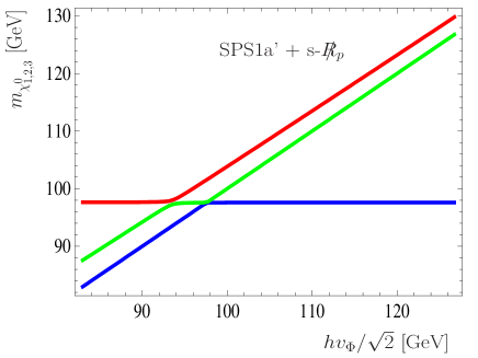
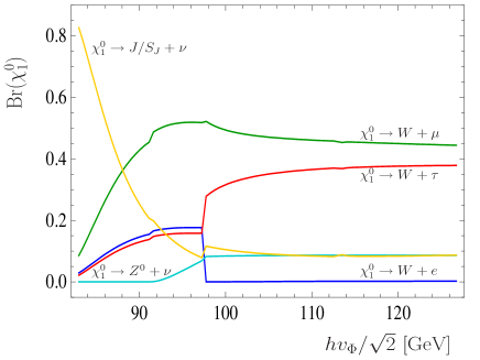
Figure 1: Masses of the three lightest neutralinos (left) and branching ratios for the most important decay modes of the lightest state (right) versus $\frac{1}{\sqrt{2}}hv_{\Phi}$ for a specific, but typical example point. The MSSM parameters have been adjusted such that the sparticle spectrum of the standard point SPS1a’ is approximately reproduced. The singlet parameters have been chosen randomly, $v_{R}=v_{S}=1$ TeV, ${\vec{\epsilon}}$ and $\vec{\Lambda}$ have been fitted to neutrino data, such that $\vec{\Lambda}$ generates the atmospheric scale and ${\vec{\epsilon}}$ the solar scale. For a detailed discussion see text.

Here we will discuss the main decay modes of bino and singlino LSPs. We will first discuss the parameter range, where $m_{\chi^{0}_{1}}\geq m_{W^{\pm}}$, such that two-body decays of $\chi^{0}_{1}$ to gauge bosons are kinematically allowed. Fig. (1) shows an example of the three lightest neutralino mass eigenvalues (left) and the main decay modes of $\chi^{0}_{1}$ (right) as a function $\frac{hv_{\Phi}}{\sqrt{2}}$ for fixed values of all other parameters. This point has been constructed in such a way, that the MSSM part of the spectrum, all production cross sections and all decay branching ratios, apart from the lightest neutralino decays, match very closely the mSugra standard point SPS1a’ AguilarSaavedra:2005pw . Here, $v_{R}=v_{S}=1$ TeV has been chosen as an arbitrary, but typical example.

The left part of fig. (1) shows how the quasi-Dirac pair ${\cal S}_{1,2}$ evolves as a function of $\frac{hv_{\Phi}}{\sqrt{2}}$. For low values (i.e. $\raise 1.29167pt\hbox{$\;<$\kern-7.5pt\raise-4.73611pt\hbox{$\sim\;$}}M_{1}$)of this parameter combination ${\cal S}_{1}$ is the LSP, for large values a ${\tilde{B}}$ is the LSP. The right side of the figure shows the final states with the largest branching ratios. For low values of the LSP mass, $J/S_{J}+\nu$ is usually the most important, i.e. there is a sizeable decay to invisible final states, even for a relatively high $v_{R}$, see also the discussion for fig. (4). Next in importance are the final states involving $W^{\pm}$ and charged leptons. Note, that the model predicts

$$\frac{\sum_{i}Br(\chi_{1}^{0}\to Z^{0}+\nu_{i})}{2\sum_{i}Br(\chi_{1}^{0}\to W^{+}+l_{i}^{-})}\simeq\frac{g}{4\cos^{2}\theta_{W}}$$ (43)

with $g$ being a phase space correction factor, with $g\to 1$ in the limit $m_{\chi^{0}_{1}}\to\infty$ Hirsch:2005ag . Equation (43) can be understood with the help of the approximative couplings eq. (29) and eq. (32). The relative size of the branching ratios for the final states $W+e$, $W+\mu$ and $W+\tau$ depends on both, (a) the nature of the LSP and (b) the fit to the neutrino data. We will discuss this important feature in more detail in section IV.

Generally, for $m_{\chi^{0}_{1}}\geq m_{W^{\pm}}$ three-body final states of the neutralino decay are less important than the two-body decays shown in fig. (1). Especially one expects that the final state $\nu b{\bar{b}}$ has a smaller branching than in the case of explicit $R_{p}/\;\>\hskip 1.99997pt$Porod:2000hv . This is essentially due to the fact, that $|\vec{\epsilon}|/\mu$ is smaller in s-$R_{p}/\;\>\hskip 1.99997pt$with a “light” singlet spectrum than in a model with explicit bilinear $R_{p}/\;\>\hskip 1.99997pt$, see the discussion in section II.3. A smaller $|\vec{\epsilon}|/\mu$ leads to smaller couplings between $\chi^{0}_{1}-l-{\tilde{l}}$, $\chi^{0}_{1}-q-{\tilde{q}}$ and especially $\chi^{0}_{1}-\nu-h^{0}$, see also couplings in Porod:2000hv . We have checked numerically, that Br($\chi^{0}_{1}\to\nu+h^{0}$), if kinematically open, is typically below $1\%$ for singlets in the ${\cal O}({\rm TeV})$ range.

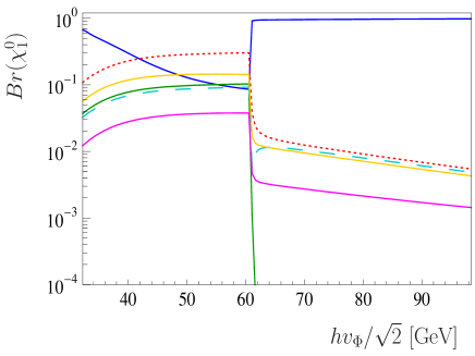
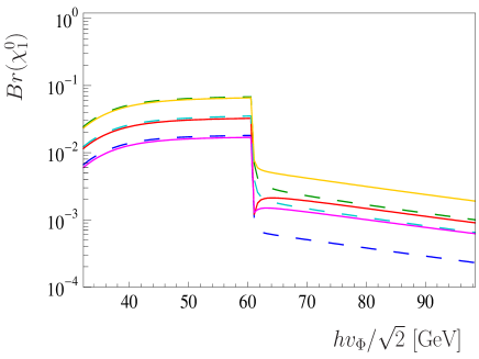
Figure 2: Branching ratios for the most important decay modes of the lightest neutralino state versus $\frac{1}{\sqrt{2}}hv_{\Phi}$ for a specific, but typical example point. The MSSM parameters have been adjusted such that the sparticle spectrum of the standard point SU4 is approximately reproduced. The singlet parameters have been chosen randomly, $v_{R}=v_{S}=1$ TeV, ${\vec{\epsilon}}$ and $\vec{\Lambda}$ have been fitted to neutrino data, such that $\vec{\Lambda}$ generates the atmospheric scale and ${\vec{\epsilon}}$ the solar scale. The different final states are as follows. In the left figure, as ordered on the right side, from top to bottom the lines are Br($\chi^{0}_{1}\to[{\rm invisible}]$) (full line, blue), Br($\chi^{0}_{1}\to\mu qq^{\prime}$) (short-dashed, red), Br($\chi^{0}_{1}\to\tau qq^{\prime}$) (large-dashed, light blue), Br($\chi^{0}_{1}\to\nu q{\bar{q}}$) (full, yellow), Br($\chi^{0}_{1}\to\nu b{\bar{b}}$) (full, pink) and Br($\chi^{0}_{1}\to eqq^{\prime}$) (full, green). In the right figure, purely leptonic modes, from top to bottom (on the right side): Br($\chi^{0}_{1}\to\nu\mu\tau$) (full, yellow), Br($\chi^{0}_{1}\to\nu e\mu$) (dashed, green), Br($\chi^{0}_{1}\to\nu e\tau$) (full, red), Br($\chi^{0}_{1}\to\nu\mu\mu$) (dashed, light blue), Br($\chi^{0}_{1}\to\nu\tau\tau$) (full, pink) and Br($\chi^{0}_{1}\to\nu ee$) (dashed, darker blue). For a detailed discussion see text.

For the case of $m_{\chi^{0}_{1}}\leq m_{W^{\pm}}$ fig. (2) shows an example for the most important final states of the lightest neutralino decay as a function of $\frac{hv_{\Phi}}{\sqrt{2}}$. As in the fig. (1) to the left the lightest neutralino is a singlino, to the right of the “transition” region the lightest neutralino is a bino. Note that the point SU4 atlas:su4 produces a bino mass of approximately $m_{\tilde{B}}\simeq 60$ GeV, thus the only two body decay modes which are kinematically allowed are $J+\nu$ and - very often, but not always - $S_{J}+\nu$. One observes that these invisible decay modes have typically a larger branching ratio than in the case $m_{\chi^{0}_{1}}\geq m_{W^{\pm}}$ shown in fig. (1). This fact is essentially due to the propagator and phase space suppression factors for three body decays. For a bino LSP the invisible decay has the largest branching fraction. Semileptonic modes are next important with typically $l_{i}qq^{\prime}$ being larger than $\nu q{\bar{q}}$. It is interesting to note, that in the purely leptonic decays, lepton flavour violating final states such as $\mu\tau$ have branching ratios typically as large or larger than the corresponding charged lepton flavour diagonal decays ($\mu\mu$ and $\tau\tau$). These large flavour off-diagonal decays can be traced to the fact that neutrino physics requires two large mixing angles. The branching ratios shown in fig. (2) should be understood only as representative examples - not as firm predictions. Especially for the case of a bino LSP, the partial width to the final state $J+\nu$, i.e. invisible final state, can vary by several orders of magnitude, see the discussion below. The predictions for relative ratios of the different (partially or completely) visible final states is much tighter fixed, because these final states correlate with neutrino physics, as we discuss in section IV.

If the ${\cal S}$ is the LSP, a bino NLSP decays dominantly to the singlino plus missing energy, as is shown in fig. (3). The final state can be either ${\cal S}_{1}+J$ or ${\cal S}_{1}+2J$, the latter due to the chain ${\tilde{B}}\to{\cal S}_{2}+J\to{\cal S}_{1}+2J$, where the 2nd step has always a branching fraction very close to $100\%$. However, a special opportunity arises if $h$ is low. In this case $\sum_{i}Br(\chi^{0}_{3}\simeq{\tilde{B}}\rightarrow W^{\pm}+l_{i}^{\mp})$ can easily reach several percent and it becomes possible to test the model with the bino decays and the singlino decays at the same time. This would allow a much more detailed study of the model parameters than for the more “standard” case where only either singlino or bino decay visibly. We note that for any fixed value of $h$, $\sum_{i}Br(\chi^{0}_{3}\simeq{\tilde{B}}\rightarrow W^{\pm}+l_{i}^{\mp})$ depends mostly on $v_{R}$ (and to some extend on $v_{\Phi}$). Low values if $v_{R}$ lead to low $\sum_{i}Br(\chi^{0}_{3}\simeq{\tilde{B}}\rightarrow W^{\pm}+l_{i}^{\mp})$ as we will discuss next.

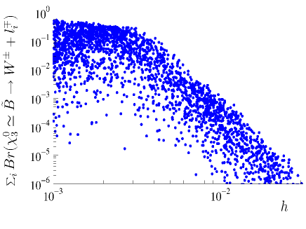
Figure 3: Sum over $\sum_{i}Br(\chi^{0}_{3}\simeq{\tilde{B}}\rightarrow W^{\pm}+l_{i}^{\mp})$ versus $h$ for MSSM parameters resembling the standard point SPS1a’, random values of the singlet parameters and with the condition of ${\cal S}_{1}$ being the LSP. The dominant decay mode for the ${\tilde{B}}$ in all points is ${\tilde{B}}\rightarrow{\cal S}_{1}+$E /  , with the missing energy due to either $J$ or 2$J$ emission. For low values of $h$ one can have visible decays of the ${\tilde{B}}$ reaching $(20-30)\%$, for $h$ larger than, for say, $h=0.05$ ${\tilde{B}}$ decays to ${\cal S}_{1}$ plus missing energy with nearly $100\%$.

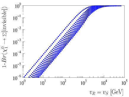
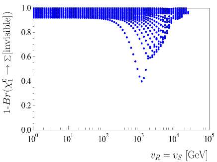
Figure 4: Sum over all at least partially visible decay modes of the lightest neutralino versus $v_{R}$ in GeV, for a set of $v_{\Phi}$ values $v_{\Phi}=10$–40 TeV for the mSUGRA parameter point $m_{0}=280$ GeV, $m_{1/2}=250$ GeV, $\tan\beta=10$, $A_{0}=-500$ GeV and $sgn(\mu)=+$. To the left $\chi_{1}^{0}\simeq{\tilde{B}}$; to the right $\chi_{1}^{0}\simeq{\cal S}$. The plot demonstrates that the branching ratio into ${\tilde{B}}\to J+\nu$ does depend strongly on the value of $v_{R}$ and to a minor extend on $v_{\Phi}$. Lowering $v_{R}$ one can get branching ratios for the invisible decay of the ${\tilde{B}}$ very close to 100 %, thus a very MSSM-like phenomenology. The right plot demonstrates that such a possibility does not exist in the case of an ${\cal S}$ LSP.

Fig. (4) shows the sum over all at least partially visible decay modes of the lightest neutralino versus $v_{R}$ in GeV, for a set of $v_{\Phi}$ values $v_{\Phi}=10$–40 TeV for the mSUGRA parameter point ($m_{0}=280$ GeV, $m_{1/2}=250$ GeV, $\tan\beta=10$, $A_{0}=-500$ GeV and sgn$(\mu)=+$). This point was constructed to produce formally a $\Omega_{\chi^{0}_{1}}h^{2}\simeq 1$ in case of conserved R-parity, much larger than the observed relic DM density Spergel:2006hy . The left plot shows the case $\chi_{1}^{0}\simeq{\tilde{B}}$, the right plot $\chi_{1}^{0}\simeq{\cal S}$. For ${\tilde{B}}$, Br(${\tilde{B}}\to J+\nu$) very close to 100 % are found for low values of $v_{R}$. This feature is independent of the mSugra parameters, see the correspoding figure in Hirsch:2006di . In this case large statistics becomes necessary to find the rare visible neutralino decays, which prove that R-parity is broken. The inconsistency between the calculated $\Omega_{\chi^{0}_{1}}h^{2}$ and the measured $\Omega_{CDM}h^{2}$ might give a first indication for a non-standard SUSY model.

Figure (4) to the right shows that the case $\chi_{1}^{0}\simeq{\cal S}$ has a very different dependence on $v_{R}$. We have checked that this feature is independent of the mSugra point. For other choices of mSugra parameters larger branching ratios for Br(${\cal S}\to J+\nu$) can be obtained, but contrary to the bino LSP case, the sum over the invisible decay branching ratios never approaches 100 %.

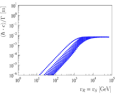
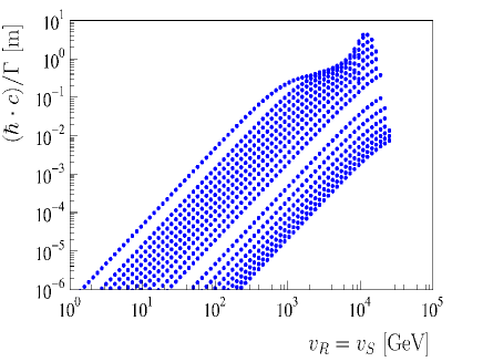
Figure 5: Decay length of the lightest neutralino in meter versus $v_{R}$. To the left: Bino LSP; to the right: Singlino LSP. All parameters have been chosen as in fig. (4).

Figure (5) shows the calculated decay lengths for the lightest neutralino for the same choice of parameters as shown in fig. (4). To the left the case $\chi_{1}^{0}\simeq{\tilde{B}}$, to the right $\chi_{1}^{0}\simeq{\cal S}$. Decay lengths depend strongly on $v_{R}$. Singlinos tend to have larger decay lengths than binos for the same choice of parameters. However, a measurement of the decay length alone is not sufficient to decide whether the LSP is a singlino or a bino. If the nature of the LSP is known, observing a finite decay length allows a rough estimate of the scale $v_{R}$, or at least to establish a rough lower limit on $v_{R}$.

Summarizing this discussion, it can be claimed that observing a decay branching ratio of the LSP into completely invisible final states larger than Br$({\chi_{1}^{0}}\to\sum[{\rm invisible}])\geq 0.1$ is an indication for s-$R_{p}/\;\>\hskip 1.99997pt$. Finding Br$({\chi_{1}^{0}}\to\sum[{\rm invisible}])\simeq 100\%$ shows furthermore that the ${\chi_{1}^{0}}$ must be a bino and measuring Br$({\chi_{1}^{0}}\to\sum[{\rm visible}])$ for a bino LSP gives an order-of-magnitude estimate of $v_{R}$.

III.3 Possible observables to distinguish between Singlino LSP and bino LSP

Since bino and singlino LSP decays have, in principle, the same final states, simply observing some visible decay products of the LSP does not allow to decide the nature of the LSP. In this subsection we will schematically discuss some possible measurements, which would allow to check for the LSP nature.

As shown above, if the singlino is the LSP and the bino the NLSP, one can have that for the bino decays to standard model particles compete with the decay to the singlino LSP. If both particles, the bino and the singlino LSP have visible decay modes, it is guaranteed that the singlino is the LSP. If the bino decays only invisibly to the singlino, a different strategy is called for. We discuss two examples in the following.

In the following discussion we will replace the neutralino mass eigenstates by the particles which correspond to their main content to avoid confusion with indices. At the LHC one will mainly produce squarks and gluinos which will decay in general in cascades. A typical example is $\tilde{q}_{L}\to q\tilde{W}$ and the wino decays further to a bino LSP as for example:

$$\tilde{W}\to e^{+}\tilde{e}^{-}\to e^{-}e^{+}\tilde{B}\to e^{-}e^{+}\mu q\bar{q}$$ (44)

$$\tilde{W}\to e^{+}\tilde{e}^{-}\to e^{-}e^{+}\tilde{B}\to e^{-}e^{+}J\nu$$ (45)

In this case one can measure in principle the neutralino mass from the first decay chain. In the invariant momentum spectrum of the $e^{+}e^{-}$ pair the edge must correspond to this mass. In the case of the singlino

$$\tilde{W}\to e^{+}\tilde{e}^{-}\to e^{-}e^{+}\tilde{B}\to e^{-}e^{+}J{\cal S}\to e^{-}e^{+}J\mu q\bar{q}$$ (46)

$$\tilde{W}\to e^{+}\tilde{e}^{-}\to e^{-}e^{+}\tilde{B}\to e^{-}e^{+}J{\cal S}\to e^{-}e^{+}JJ\nu$$ (47)

In this case one has on average more missing energy than for a bino LSP. However, in both cases one can study spectra combining the jet stemming from the squark and the $e^{+}e^{-}$ pair and obtain information on the masses from the so-called edge variables Allanach:2000kt . In addition one can use additional variables like, for example, $m_{T2}$ Barr:2003rg ; Barr:2007hy ; Cho:2007dh to obtain information on the LSP mass. Note, that this variable works also if there are additional massless particles involved, although at the expense of available statistics Barr:private . In addition one can obtain the invariant mass of the LSP from the final state $\mu q\bar{q}$. In the case where the LSP has a decay length measurable at the LHC, one can separate the latter decay products from the other particles in the event and, thus, reduce considerably the combinatorial problems associated with the correct assignment of the jets. In the case of a bino LSP one would find that all the three different measurements yield the same mass for the LSP. In the case of a singlino LSP, on the other hand, one would obtain that the LSP mass reconstructed from the edge variables does not coincide with the mass reconstructed from the $\mu q\bar{q}$ spectrum. This would indicate that there are two different particles involved. (Such a difference might also be visible in the $m_{T2}$ variable.) However, in all cases detailed Monte Carlo studies will be necessary to work out the required statistics, etc.

Distinguishing bino and singlino LSPs will become considerably easier at a future international linear collider. In $e^{+}e^{-}$ one can directly produce a bino LSP but not a singlino LSP and, thus, the identification of the correct scenario should be fairly straightforward.

IV Correlations between LSP decays and neutrino mixing angles

Correlations between LSP decays and neutrino mixing angles depend on the nature of the LSP. Above we have discussed some possible measurements which, at least in principle, allow to distinguish bino from singlino LSPs. In this subsection we assume that the nature of the LSP is known.

IV.0.1 Bino LSP

We note that the following discussion is valid also if the bino is the NLSP which, as discussed above, decays with some final, but probably small percentage to visible final states.

In explicit bilinear R-parity violation the coupling of the bino component of the neutralino to gauge bosons and leptons is completely dominated by terms proportional to $\Lambda_{i}$, as has been shown in Porod:2000hv . Although the coefficients for the spontaneous model are more complicated, see the discussion in section II.4, generation dependence for the coefficients for the coupling $\chi_{1}^{0}-W-l_{i}$ appear only in the terms $\Lambda_{i}$ and $\epsilon_{i}$, i.e. $K_{\Lambda}^{i}$ and $K_{\epsilon}^{i}$ are independent of the lepton generation. Numerically one finds than that the terms proportional to $\Lambda_{i}$ dominate the $\chi_{1}^{0}-W-l_{i}$ coupling for a bino LSP always. This is demonstrated in figs. (6) and (7). Here we have numerically scanned the mSugra parameter space, with random singlet parameters and the additional condition that the LSP is a bino. For the left (right) figures we have numerically applied the cut $N_{11}^{2}>0.5$ ($N_{11}^{2}>0.9$).

Fig. (6) [ (7)] shows the ratio of branching ratios Br(${\tilde{B}}\to W+e$)/Br(${\tilde{B}}\to W+\mu$) [Br(${\tilde{B}}\to W+\mu$)/Br(${\tilde{B}}\to W+\tau$)] versus $(\Lambda_{e}/\Lambda_{\mu})^{2}$ [$(\Lambda_{\mu}/\Lambda_{\tau})^{2}$]. To establish a correlation between ratios of $\Lambda_{i}$ and the bino decay branching ratios, a bino purity of $N_{11}^{2}>0.5$ is usually sufficient. The figures demonstrate that the correlations get sharper with increasing bino purity.

We have checked that for neutralinos with mass lower than $m_{W}$ one can use ratios of the decays ${\tilde{B}}\rightarrow l_{i}qq^{\prime}$ for the different $l_{i}$ in the same way to perform a measurement of $\Lambda_{i}$ ratios. Plots for this parameter region are rather similar to the ones shown for the case ${\tilde{B}}\rightarrow l_{i}W$, although with a somewhat larger dispersion, and we therefore do not repeat them here.

With the measurement of ratios of branching ratios different consistency checks of the model can be performed. In case (c1), i.e. $\vec{\Lambda}$ explaining the atmospheric scale, the atmospheric and the reactor angle are related to $W+l$ final states, as shown in fig. (8). Here we show the ratios ${\cal R}_{\mu}=\frac{Br(\chi^{0}_{1}\rightarrow\mu W)}{Br(\chi^{0}_{1}\rightarrow\tau W)}$ versus $\tan^{2}\theta_{Atm}$ (left) and ${\cal R}_{e}=\frac{Br(\chi^{0}_{1}\rightarrow eW)}{\sqrt{Br(\chi^{0}_{1}\rightarrow\mu W)^{2}+Br(\chi^{0}_{1}\rightarrow\tau W)^{2}}}$ versus $\sin^{2}\theta_{R}$ (right) for a bino LSP, for an assumed bino-purity of $N_{11}^{2}>0.8$. The vertical lines are the $3\sigma$ c.l. allowed experimental ranges (upper bound), horizontal lines the resulting predictions for the two different observables ${\cal R}$. Given the current experimental data, one expects $\frac{Br(\chi^{0}_{1}\rightarrow\mu W)}{Br(\chi^{0}_{1}\rightarrow\tau W)}$ in the range $[0.4,2.1]$ and $\frac{Br(\chi^{0}_{1}\rightarrow eW)}{\sqrt{Br(\chi^{0}_{1}\rightarrow\mu W)^{2}+Br(\chi^{0}_{1}\rightarrow\tau W)^{2}}}\leq 0.06$.

Different from fig. (8), in case of (c2), i.e. $\vec{\Lambda}$ explaining the solar scale, the ratio $\frac{Br(\chi^{0}_{1}\rightarrow eW)}{\sqrt{Br(\chi^{0}_{1}\rightarrow\mu W)^{2}+Br(\chi^{0}_{1}\rightarrow\tau W)^{2}}}$ correlates with $\tan^{2}\theta_{\odot}$, as shown in fig. (9). Here, from the $3\sigma$ c.l. allowed range of the solar angle one expects to find $\frac{Br(\chi^{0}_{1}\rightarrow eW)}{\sqrt{Br(\chi^{0}_{1}\rightarrow\mu W)^{2}+Br(\chi^{0}_{1}\rightarrow\tau W)^{2}}}\simeq[0.25,0.85]$. Finding this ratio experimentally to be larger than the one indicated by the solar data, i.e. $\frac{Br(\chi^{0}_{1}\rightarrow eW)}{\sqrt{Br(\chi^{0}_{1}\rightarrow\mu W)^{2}+Br(\chi^{0}_{1}\rightarrow\tau W)^{2}}}>>1$, rules out the model as the origin of the observed neutrino oscillation data. Similarly a low (high) experimental value for this ratio indicates (for a bino LSP) that case (c1) [(c2)] is the correct explanation for the two observed neutrino mass scales.

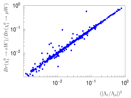
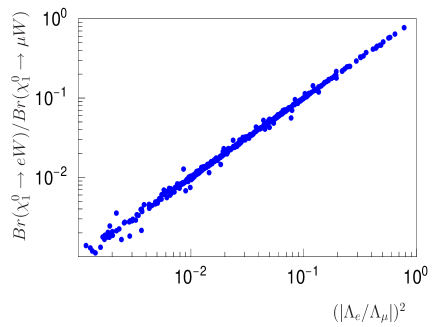
Figure 6: Ratio $\frac{Br(\chi^{0}_{1}\rightarrow eW)}{Br(\chi^{0}_{1}\rightarrow\mu W)}$ versus $(\Lambda_{e}/\Lambda_{\mu})^{2}$ for a bino LSP. To the left: “Bino-purity” $N_{11}^{2}>0.5$, to the right: $N_{11}^{2}>0.9$. All points with $m_{LSP}>m_{W}$.

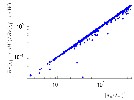
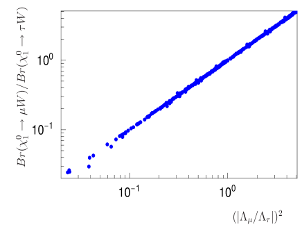
Figure 7: Ratio $\frac{Br(\chi^{0}_{1}\rightarrow\mu W)}{Br(\chi^{0}_{1}\rightarrow\tau W)}$ versus $(\Lambda_{\mu}/\Lambda_{\tau})^{2}$ for a bino LSP. To the left: “Bino-purity” $N_{11}^{2}>0.5$, to the right: $N_{11}^{2}>0.9$.

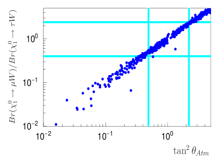
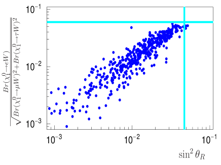
Figure 8: Ratio ${\cal R}_{\mu}=\frac{Br(\chi^{0}_{1}\rightarrow\mu W)}{Br(\chi^{0}_{1}\rightarrow\tau W)}$ versus $\tan^{2}\theta_{Atm}$ (left) and ${\cal R}_{e}=\frac{Br(\chi^{0}_{1}\rightarrow eW)}{\sqrt{Br(\chi^{0}_{1}\rightarrow\mu W)^{2}+Br(\chi^{0}_{1}\rightarrow\tau W)^{2}}}$ versus $\sin^{2}\theta_{R}$ (right) for a bino LSP. “Bino-purity” $N_{11}^{2}>0.8$. Vertical lines are the $3\sigma$ c.l. allowed experimental ranges, horizontal lines the resulting predictions for the fit (c1), see text.

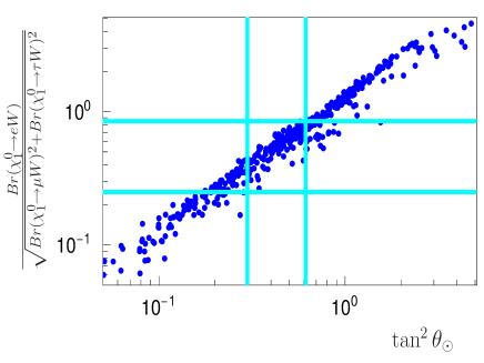
Figure 9: Ratio ${\cal R}_{e}=\frac{Br(\chi^{0}_{1}\rightarrow eW)}{\sqrt{Br(\chi^{0}_{1}\rightarrow\mu W)^{2}+Br(\chi^{0}_{1}\rightarrow\tau W)^{2}}}$ versus $\tan^{2}\theta_{\odot}$ for a bino LSP. “Bino-purity” $N_{11}^{2}>0.8$. Vertical lines are the $3\sigma$ c.l. allowed experimental ranges, horizontal lines the resulting predictions for the fit (c2), see text.

IV.0.2 Singlino LSP

Different from the bino LSP case, for singlinos coupling to a lepton $l_{i}$-W pair terms proportional to $\epsilon_{i}$ dominate by far. This is demonstrated in fig. (10), where we show the ratios $\frac{Br(\chi^{0}_{1}\rightarrow eW)}{Br(\chi^{0}_{1}\rightarrow\mu W)}$ (left) versus $(\epsilon_{e}/\epsilon_{\mu})^{2}$ and $\frac{Br(\chi^{0}_{1}\rightarrow\mu W)}{Br(\chi^{0}_{1}\rightarrow\tau W)}$ (right) versus $(\epsilon_{\mu}/\epsilon_{\tau})^{2}$ for a singlino LSP. Note that mixing between singlinos and the doublet neutralinos of the model is always very small, unless the singlino is highly degenerate with the bino. Consequently singlinos are usually very “pure” singlinos and the correlations of the $l_{i}$-W with the $\epsilon_{i}$ ratios is very sharp.

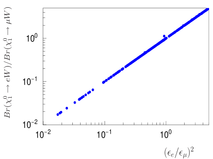
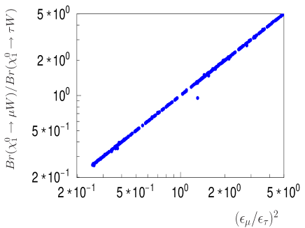
Figure 10: Ratio $\frac{Br(\chi^{0}_{1}\rightarrow eW)}{Br(\chi^{0}_{1}\rightarrow\mu W)}$ (left) versus $(\epsilon_{e}/\epsilon_{\mu})^{2}$ and $\frac{Br(\chi^{0}_{1}\rightarrow\mu W)}{Br(\chi^{0}_{1}\rightarrow\tau W)}$ (right) versus $(\epsilon_{\mu}/\epsilon_{\tau})^{2}$ for a “singlino” LSP.

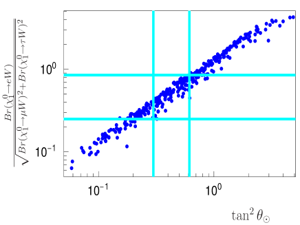
Figure 11: Ratio ${\cal R}_{e}=\frac{Br(\chi^{0}_{1}\rightarrow eW)}{\sqrt{Br(\chi^{0}_{1}\rightarrow\mu W)^{2}+Br(\chi^{0}_{1}\rightarrow\tau W)^{2}}}$ versus $\tan^{2}\theta_{\odot}$ for a singlino LSP. Vertical lines are the $3\sigma$ c.l. allowed experimental ranges, horizontal lines the resulting predictions for the fit (c1), see text.

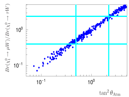
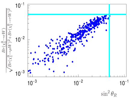
Figure 12: Ratio ${\cal R}_{\mu}=\frac{Br(\chi^{0}_{1}\rightarrow\mu W)}{Br(\chi^{0}_{1}\rightarrow\tau W)}$ versus $\tan^{2}\theta_{Atm}$ (left) and ${\cal R}_{e}=\frac{Br(\chi^{0}_{1}\rightarrow eW)}{\sqrt{Br(\chi^{0}_{1}\rightarrow\mu W)^{2}+Br(\chi^{0}_{1}\rightarrow\tau W)^{2}}}$ versus $\sin^{2}\theta_{R}$ (right) for a singlino LSP. Vertical lines are the $3\sigma$ c.l. allowed experimental ranges, horizontal lines the resulting predictions for the fit (c2), see text.

Depending on which case, (c1) or (c2), is chosen to fit the neutrino data, the corresponding ratios of branching ratios are then either sensitive to the atmospheric and reactor or the solar angle. This is demonstrated in figs. (11) and (12). Here, fig. (11) shows the correlation of ${\cal R}_{e}=\frac{Br(\chi^{0}_{1}\rightarrow eW)}{\sqrt{Br(\chi^{0}_{1}\rightarrow\mu W)^{2}+Br(\chi^{0}_{1}\rightarrow\tau W)^{2}}}$ with $\tan^{2}\theta_{\odot}$ for the fit (c1). This result is very similar to the one obtained for the fit (c2) and a bino LSP. For this reason the nature of the LSP needs to be known, before one can decide, whether the measurement of a ratio of branching ratio is testing (c1) or (c2).

Figure (12) shows the dependence of ${\cal R}_{\mu}=\frac{Br(\chi^{0}_{1}\rightarrow\mu W)}{Br(\chi^{0}_{1}\rightarrow\tau W)}$ versus $\tan^{2}\theta_{Atm}$ (left) and ${\cal R}_{e}=\frac{Br(\chi^{0}_{1}\rightarrow eW)}{\sqrt{Br(\chi^{0}_{1}\rightarrow\mu W)^{2}+Br(\chi^{0}_{1}\rightarrow\tau W)^{2}}}$ versus $\sin^{2}\theta_{R}$ (right) for a singlino LSP, using the neutrino fit (c2). Again one observes that this result is very similar to the one obtained for a bino LSP and fit (c1). This simply reflects that fact, that neutrino angles can be either fitted with ratios of $\epsilon_{i}$ or with ratios of $\Lambda_{i}$ and singlinos couple mostly proportional to $\epsilon_{i}$, while binos are sensitive to $\Lambda_{i}$.

In case the singlino is the LSP and the bino, as the NLSP, decays with some measurable branching ratios to $W-l_{i}$, both $\Lambda_{i}$ and $\epsilon_{i}$ ratios could be reconstructed, which would allow for a much more comprehensive test of the model.

V Conclusions

We have studied the phenomenology of a neutralino LSP in a supersymmetric model in which neutrino oscillation data is explained by spontaneous R-parity violation. We have concentrated the discussion on the case that the LSP is either a bino, like in a typical mSugra point, or a singlino state, novel to the current model. We have worked out the most important phenomenological signals of the model and how it might be distinguished from the well-studied case of the MSSM, as well as from a model in which the violation of R-parity is explicit.

There are regions in parameter space, where $\tilde{\chi}^{0}$ decays invisibly with branching ratios close to 100 %, despite the smallness of neutrino masses. In this limit, spontaneous violation of R-parity can resemble the MSSM with conserved R-parity at the LHC and experimentalist would have to search for the very rare visible decay channels to establish the R-parity indeed is broken.

The perhaps most important test of the model as the origin of the observed neutrino masses comes from measurements of ratios of branching ratios to $W$-boson and charged lepton final states. Ratios of these decays are always related to measured neutrino angles. If SUSY has a spectrum light enough to be produced at the LHC, the spontaneous model of R-parity violation is therefore potentially testable.

References

- (1) Super-Kamiokande, Y. Fukuda et al., Phys. Rev. Lett. 81, 1562 (1998), [hep-ex/9807003].
- (2) SNO, Q. R. Ahmad et al., Phys. Rev. Lett. 89, 011301 (2002), [nucl-ex/0204008].
- (3) KamLAND, K. Eguchi et al., Phys. Rev. Lett. 90, 021802 (2003), [hep-ex/0212021].
- (4) [MINOS Collaboration], arXiv:0708.1495 [hep-ex].
- (5) KamLAND Collaboration, arXiv:0801.4589 [hep-ex].
- (6) M. Maltoni, T. Schwetz, M. A. Tortola and J. W. F. Valle, New J. Phys. 6, 122 (2004); Online version 6 in arXiv:hep-ph/0405172 contains updated fits with data included up to Sep 2007.
- (7) P. Minkowski, Phys. Lett. B67, 421 (1977).
- (8) T. Yanagida, In Proceedings of the Workshop on the Baryon Number of the Universe and Unified Theories, Tsukuba, Japan, 13-14 Feb 1979.
- (9) M. Gell-Mann, P. Ramond and R. Slansky, Print-80-0576 (CERN), Proceedings of the Workshop, Stony Brook, NY (North-Holland, Amsterdam, 1979).
- (10) R. N. Mohapatra and G. Senjanovic, Phys. Rev. Lett. 44, 912 (1980).
- (11) J. Schechter and J. W. F. Valle, Phys. Rev. D22, 2227 (1980).
- (12) F. Deppisch, H. Pas, A. Redelbach, R. Ruckl and Y. Shimizu, Eur. Phys. J. C 28, 365 (2003) [arXiv:hep-ph/0206122].
- (13) G. A. Blair, W. Porod and P. M. Zerwas, Eur. Phys. J. C27, 263 (2003), [hep-ph/0210058].
- (14) A. Freitas, W. Porod and P. M. Zerwas, Phys. Rev. D72, 115002 (2005), [hep-ph/0509056].
- (15) M. R. Buckley and H. Murayama, Phys. Rev. Lett. 97, 231801 (2006) [arXiv:hep-ph/0606088].
- (16) F. Deppisch, A. Freitas, W. Porod and P. M. Zerwas, arXiv:0712.0361 [hep-ph].
- (17) K. S. Babu, Phys. Lett. B203, 132 (1988).
- (18) D. Aristizabal Sierra, M. Hirsch and S. G. Kovalenko, arXiv:0710.5699 [hep-ph].
- (19) L. J. Hall and M. Suzuki, Nucl. Phys. B231, 419 (1984).
- (20) For a review on bilinear R-parity violation see, M. Hirsch and J. W. F. Valle, New J. Phys. 6, 76 (2004) [arXiv:hep-ph/0405015].
- (21) W. Porod, M. Hirsch, J. Romão and J. W. F. Valle, Phys. Rev. D63, 115004 (2001), [hep-ph/0011248].
- (22) D. Restrepo, W. Porod and J. W. F. Valle, Phys. Rev. D64, 055011 (2001), [hep-ph/0104040].
- (23) M. Hirsch, W. Porod, J. C. Romão and J. W. F. Valle, Phys. Rev. D66, 095006 (2002), [hep-ph/0207334].
- (24) A. Bartl, M. Hirsch, T. Kernreiter, W. Porod and J. W. F. Valle, JHEP 11, 005 (2003), [hep-ph/0306071].
- (25) M. Hirsch and W. Porod, Phys. Rev. D68, 115007 (2003), [hep-ph/0307364].
- (26) D. N. Spergel et al. [WMAP Collaboration], Astrophys. J. Suppl. 170, 377 (2007) [arXiv:astro-ph/0603449].
- (27) S. Borgani, A. Masiero and M. Yamaguchi, Phys. Lett. B 386, 189 (1996) [arXiv:hep-ph/9605222].
- (28) F. Takayama and M. Yamaguchi, Phys. Lett. B485, 388 (2000), [hep-ph/0005214].
- (29) M. Hirsch, W. Porod and D. Restrepo, JHEP 03, 062 (2005), [hep-ph/0503059].
- (30) J. E. Kim, Phys. Rept. 150, 1 (1987).
- (31) G. G. Raffelt, Stars as Laboratories for Fundamental Physics (University of Chicago, Chicago, 1996) p. 664.
- (32) E. J. Chun and H. B. Kim, Phys. Rev. D60, 095006 (1999), [hep-ph/9906392].
- (33) M. Hirsch, PoS HEP2005, 343 (2006).
- (34) M. Hirsch and W. Porod, Phys. Rev. D 74, 055003 (2006) [arXiv:hep-ph/0606061].
- (35) C. S. Aulakh and R. N. Mohapatra, Phys. Lett. B119, 136 (1982).
- (36) A. Masiero and J. W. F. Valle, Phys. Lett. B251, 273 (1990).
- (37) Particle Data Group, W. M. Yao et al., J. Phys. G33, 1 (2006).
- (38) R. Barbieri, S. Ferrara and C. A. Savoy, Phys. Lett. B119, 343 (1982).
- (39) M. Hirsch, J. C. Romao, J. W. F. Valle and A. Villanova del Moral, Phys. Rev. D70, 073012 (2004), [hep-ph/0407269].
- (40) M. Hirsch, J. C. Romao, J. W. F. Valle and A. Villanova del Moral, Phys. Rev. D73, 055007 (2006), [hep-ph/0512257].
- (41) F. Franke and S. Hesselbach, Phys. Lett. B 526, 370 (2002) [arXiv:hep-ph/0111285].
- (42) M. Hirsch, M. A. Díaz, W. Porod, J. C. Romão and J. W. F. Valle, Phys. Rev. D62, 113008 (2000), [hep-ph/0004115].
- (43) J. C. Romão, M. A. Díaz, M. Hirsch, W. Porod and J. W. F. Valle, Phys. Rev. D61, 071703 (2000), [hep-ph/9907499].
- (44) M. A. Díaz, M. Hirsch, W. Porod, J. C. Romão and J. W. F. Valle, Phys. Rev. D68, 013009 (2003), [hep-ph/0302021].
- (45) P. F. Harrison, D. H. Perkins and W. G. Scott, Phys. Lett. B 530 (2002) 167 [arXiv:hep-ph/0202074].
- (46) B. Mukhopadhyaya, S. Roy and F. Vissani, Phys. Lett. B 443, 191 (1998) [arXiv:hep-ph/9808265].
- (47) S. Y. Choi, E. J. Chun, S. K. Kang and J. S. Lee, Phys. Rev. D 60, 075002 (1999) [arXiv:hep-ph/9903465].
- (48) F. de Campos, O. J. P. Eboli, M. B. Magro, W. Porod, D. Restrepo, M. Hirsch and J. W. F. Valle, arXiv:0712.2156 [hep-ph].
- (49) W. Porod, Comput. Phys. Commun. 153, 275 (2003) [arXiv:hep-ph/0301101].
- (50) J. A. Aguilar-Saavedra et al., Eur. Phys. J. C 46, 43 (2006) [arXiv:hep-ph/0511344].
-
(51)
ATLAS collaboration, Rome meeting, 2004,
https://twiki.cern.ch/twiki/bin/view/Atlas/RomeSUSYWiki - (52) B. C. Allanach, C. G. Lester, M. A. Parker and B. R. Webber, JHEP 0009 (2000) 004 [arXiv:hep-ph/0007009].
- (53) A. Barr, C. Lester and P. Stephens, J. Phys. G 29 (2003) 2343 [arXiv:hep-ph/0304226].
- (54) A. J. Barr, B. Gripaios and C. G. Lester, arXiv:0711.4008 [hep-ph].
- (55) W. S. Cho, K. Choi, Y. G. Kim and C. B. Park, arXiv:0711.4526 [hep-ph].
- (56) A. J. Barr, private communications.