The Ionizing Stars of the Galactic Ultra–Compact H II Region G45.45$+$0.06

Abstract

Using the NIFS near–infrared integral–field spectrograph behind the facility adaptive optics module, ALTAIR, on Gemini North, we have identified several massive O–type stars that are responsible for the ionization of the Galactic Ultra–Compact H II region G45.45$+$0.06. The sources “m” and “n” from the imaging study of Feldt et al. (1998) are classified as hot, massive O–type stars based on their $K-$band spectra. Other bright point sources show red and/or nebular spectra and one appears to have cool star features that we suggest are due to a young, low–mass pre–main sequence component. Still two other embedded sources (“k” and “o” from Feldt et al.) exhibit CO bandhead emission that may arise in circumstellar disks which are possibly still accreting. Finally, nebular lines previously identified only in higher excitation planetary nebulae and associated with Kr III and Se IV ions are detected in G45.45$+$0.6.

Facilities: Gemini:Gillett ()

1 Introduction

G45.45$+$0.06 is a luminous ultra–compact H II (UCH II) region identified by Wood & Churchwell (1989) as a “cometary” type in their landmark radio survey. UCH II regions have become synonymous with the earliest phases of massive star birth (Churchwell, 2002) and the phase in which the object is first revealed as an identifiable hot, massive star as evidenced by its strong ionizing radiation. Wood & Churchwell (1989) noted that many of the UCH II regions must be excited by multiple sources, in effect harboring clusters of stars. This has indeed turned out to be the case. Feldt et al. (1998) presented high angular resolution near infrared images of G45.45$+$0.06 that showed multiple point sources and a complex morphology.

We have used the new Near–infrared Integral–Field Spectrograph (NIFS) on the Gemini North Fredrick C. Gillett 8–m telescope to carry out a detailed investigation of this UCH II region and build on the Feldt et al. (1998) imaging study. UCH II regions typically have sizes $\mathrel{\hbox{\hbox to0.0pt{\hbox{\lower 4.0pt\hbox{$\sim$}}\hss}\hbox{$<$}}}$0.1 pc. At the distance of G45.45$+$0.06 (Feldt et al., 1998, 6.6 kpc) this scale just fills the NIFS three arc second field. Using the facility adaptive optics module ALTAIR with NIFS, we obtained $\sim$ 0.1^′′ images in several pointings in the larger Feldt et al. (1998) field. Adaptive optics on large aperture telescopes offers a significant advance in the study of massive stars in their earliest phases since the high angular resolution improves the point source contrast against the strong and variable nebular background. NIFS has the added benefit of a new generation 2048$\times$2048 HgCdTe array that provides broad spectral coverage (an entire near–infrared band) at medium spectral resolution ($R=$ 5000).

Previous studies of UCH II region central ionizing sources in the near–infrared have identified hot stars (Watson & Hanson, 1997; Hanson et al., 2002; Bik et al., 2005) by their photospheric features. These studies provide important constraints on the statistics of the youngest phase of massive stellar populations. Coupling such studies to integral–field observations will advance our understanding of the embedded stellar sources as well, but the added high angular resolution imaging dimension will allow for detailed modeling of ionized (and molecular) gas as well as the clustering characteristics on the smallest scales. Messineo et al. (2007) have presented results for the Galactic UCH II region [DBS2003]8 based on similar observations to those described here and made with the ESO VLT SINFONI integral–field unit spectrograph.

2 Observations

Data were obtained with NIFS at the Cassegrain focus of the Gemini North Fredrick C. Gillett 8–m telescope on Mauna Kea, Hawaii on the nights of 22 and 23 July, 2006 (local time). NIFS was used with the facility adaptive optics (AO) module ALTAIR in natural guide star (NGS) mode.

NIFS slices an approximately three arc second by three arc second field into 29 spectral segments of 0.1^′′ width (the “slit” width) and $\sim$ three arc seconds in length.The scale along the spatial dimension is 0.043^′′ pix^-1. The resulting “spaxels” are thus 0.043^′′ $\times$ 0.1^′′, and each contains a full spectrum covering one of the near–infrared bands. See McGregor et al. (2003) for a complete description of NIFS.

In the present case, $K-$band spectra are presented for G45.45$+$0.6 for two pointings from the field described by Feldt et al. (1998). The two pointings were chosen to include candidate ionizing sources identified by Feldt et al. (1998).The AO guide star used for ALTAIR is located about 12^′′ to the north and east from the two NIFS pointings. The AO guide star has an $R$ magnitude of 11.8 according to the USNO catalog (source id: U0975_14397240). The conditions were sufficient with the AO correction to isolate all the point sources identified by Feldt et al. (1998) within the NIFS field of view. On the 22nd of July, the sky was clear, and the seeing (at 5000 Å) during the observations (pointing 1) was approximately 0.6${}^{\prime\prime}--0.8^{\prime\prime}$, and the observations were obtained at relatively high airmass (1.6–1.9). ALTAIR was run at 500 Hz for these observations. On July 23rd, there were thin clouds and the seeing was again about 0.6${}^{\prime\prime}--0.8^{\prime\prime}$ but this time for an observation airmass near 1.0 (pointing 2). ALTAIR was run at 100 Hz for these observations due to the clouds.

Each pointing consisted of a set of undithered frames taken on source as well as a sky frame obtained on a nearby ($\sim$ 50^′′ West) blank field. The pointings had total exposure times of 1800 seconds (3$\times$600s) on source and 600 seconds on sky. At the time of the observations, shortly after NIFS commissioning, it was judged best to stare on source to simplify combining of the frames in the post–observation reduction. NIFS has a 2048$\times$2048 HgCdTe detector (HAWAII–2RG) with a significant number of hot pixels that were removed by sky subtraction. Current NIFS observations are best taken with small dithers to help reduce the effect of the hot pixels. The relatively long exposures used to reach near–sky–noise–limited performance also result in significant numbers of cosmic rays. These can be mitigated by multiple exposures as well. The NIFS dark current is quite low, apart from hot pixels, and is measured to be $\mathrel{\hbox{\hbox to0.0pt{\hbox{\lower 4.0pt\hbox{$\sim$}}\hss}\hbox{$<$}}}$0.1 e^- s^-1. The RMS read noise is approximately six e^- in low noise mode which uses multiple reads of the detector.

The spectral resolving power of NIFS in the $K-$band is $\lambda/\Delta\lambda=$ 5160 which results in a linear dispersion of 2.13 Å/pixel. This dispersion, combined with the large format array gives a full wavelength coverage at $K$ of about 4200 Å accounting for some minor truncation in the final data cube due to the systematic shift of wavelength in each slitlet from the staircase design of the image slicer.

3 Data Reduction

The line maps and spectra presented here were obtained using the Gemini NIFS IRAF data reduction package (version 1.9).

The NIFS IRAF package allows for full reduction to the “image cube” stage where a finalcube has a roughly 60$\times$62 pixel image plane and a 2040 pixel spectral depth. First, raw images are prepared for reduction by standard Gemini procedures that create the FITS image variance and data quality extensions. Next, the data are sky subtracted, flatfielded, rectified spatially, and wavelength calibrated. The last two steps result in a uniform spatial–spectral trace for each image slice row and a linear wavelength scale. It is important to remember that the final IRAF data cube resamples each slitlet to two 0.05^′′ pixels for convenience; the angular resolution in this dimension is still 0.1^′′. It might be possible to enhance the resolution in the slitlet spatial dimmension by careful dithering of the telescope and combining of the data, but this is not the default situation for NIFS that provides native 0.048^′′ $\times$ 0.1^′′ “pixels” on the sky.

The spatial rectification was accomplished by use of a Ronchi mask image taken as part of the baseline calibration set for NIFS. The Ronchi mask is a coarse transmission grating deployed in the instrument focal plane and illuminated by the flatfield calibration lamp. It produces a uniform distribution of compact artifical sources along each image slice. In the spatial dimension, the Ronchi mask produces nine spectral traces for each slice. Each trace can be thought of as the trace of a point source at a given spatial position of each slice. Fitting the traces for all slices primarily removes a small systematic ($\sim$ $\pm$ one pixel end–to–end) slope of the spectral trace and allows for an accurate reconstruction of the 2–D image since the traces of one slice can be identified with the traces of neighboring slices.

A lamp image of Ar and Xe lines was used to determine the dispersion along each slice and as a function of the spatial dimension of each slice. A quadratic polynomial was used in this case which produced typical uncertainties in the position of a spectral line of approximately $\pm$ 0.2 Å ($\sim$ 1/10 pixel). Final spectra are interpolated to a linear wavelength solution.

The spectra were next corrected for telluric absorption by division by the spectrum of an A0 V star. Each A0 V (in this case HIP84147 and HIP89309 on July 22 and HIP99796 on July 23) was corrected for intrinsic Br$\gamma$ absorption by fitting a Voigt profile to the telluric spectrum. This approximate correction is sufficient for our purposes since the hot star photospheric classifications do not rely on Br$\gamma$.

The fully rectified and telluric corrected images were used to extract point sources using the NFEXTRACT routine. In the Gemini IRAF NIFS package, the point source extraction is done on the image that still contains the 29 slices, i.e. before construction of a final data cube image (the extraction aperture is applied to a temporary cube). In this case, the NFEXTRACT routine was modified to allow for a secondary sky spectrum to be subtracted from the point source to account for over– or under–subtraction of sky between the on–source and sky images. In both G45.45$+$0.06 pointings, a one arc second diameter aperture was used to measure the residual sky emission. This aperture obviously includes some nebular emission, but the sky aperture location was chosen to minimize this effect. For pointing 1, this was a location to the South and West of the point sources near the edge of the image (see below). For pointing 2, the sky aperture was located to the North and West of the point sources near the edge of the image. All point sources were extracted using a 0.4^′′ diameter aperture. This aperture was chosen to minimize the overlap between point sources while attempting to obtain as much flux as possible and is distinguished from the larger aperture used for flux calibration (see next) that was chosen to match the photometry of Feldt et al. (1998).

The final wavelength calibrated, spatially rectified, and telluric corrected images were transformed into data cubes. The spatial pixel scale was interpolated to 0.05^′′ in the fine dimension and block replicated to 0.05^′′ in the course dimension providing for a uniform scale as described in the previous section. Line maps presented below were extracted from these cubes using NFMAP. A rough flux calibration was done by extracting spectra in 0.5^′′ apertures and comparing them to the photometry of Feldt et al. (1998) from the same diameter aperture (source “o” in pointing 1, and sources “g”, ”h”, ”i”, and “k” in pointing two). No attempt was made to correct the fraction of light outside this aperture in the seeing halo for this approximate flux calibration. Making an aperture correction on the science frames is not possible because of the strong nebular emission; however, the standard stars taken before and after the science observations (under similar seeing as the science targets) suggest that a 0.5^′′ diameter aperture misses at least 25$\%$ of the stellar flux. The following results and discussion do not depend strongly on the absolute calibration of the NIFS data. This calibration applies only to the extended emission maps presented below; point sources are calibrated directly to the Feldt et al. (1998) $K^{\prime}$ magnitudes ($\lambda_{\circ}=$2.12 $\mu$m) using a flux zero point of 4.75$\times$10^-11 erg cm^-2-s^-1-Å^-1. This gives $Ks$ ($\approx$ $K$) $=$ 12.4 and 12.0 mag for sources “m” and “n”, respectively.

4 Results

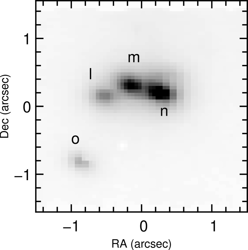
Figure 1: Continuum map at 21695 Å (10.7 Å wide) for the first NIFS pointing. The point sources are labeled following Feldt et al. (1998). Sources m and n exhibit spectra of mid O–type stars while source “o” has CO band head emission at 2.3 $\mu$m suggesting it may be a massive young stellar object; see text and Figures 3 and 5. The field center is located at approximately RA(2000)$=$19$h$ 14$m$ 21.24$s$, Dec(2000)$=+$11$d$ 09^′ 10.1^′′. North is up and East to the left in the image, as indicated.

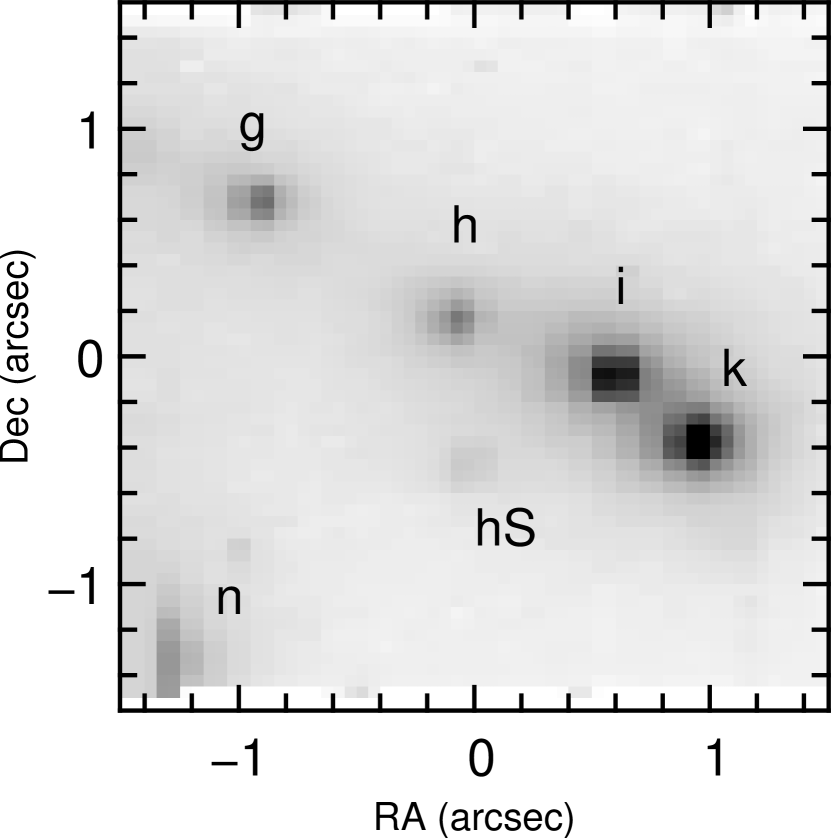
Figure 2: Continuum map at 21695 Å (10.7 Å wide) for the second NIFS pointing (Figure 2). The point sources are labeled following Feldt et al. (1998); “hS” is newly identified in this work. Sources “g”, ”h” and ”i” exhibit spectra with featureless red continua and source ”k” shows CO band head emission similar to source ”o”; see text and Figures 4 and 5. The field center is located at approximately RA(2000)$=$19$h$ 14$m$ 21.14$s$, Dec(2000)$=+$11$d$ 09^′ 11.9^′′. North is up and East to the left in the image, as indicated.

Figures 1 and 2 show continuum emission for pointings one and two, respectively, extracted from the final data cubes. The wavelength for the extracted band is 21695 Å, and the band is approximately 10.7 Å wide. The point sources in these images have image cores of about 0.15^′′-0.25^′′. This is for a final set of three combined images. The point source designations of Feldt et al. (1998) are indicated in each figure, and all of them are clearly and easily separated, even though they are deeply embedded in strong nebular emission from the UCH II region. A faint source not identified by Feldt et al. (1998) appears about 0.5^′′ south of source “h” in Figure 2; we designate this source “hS”.

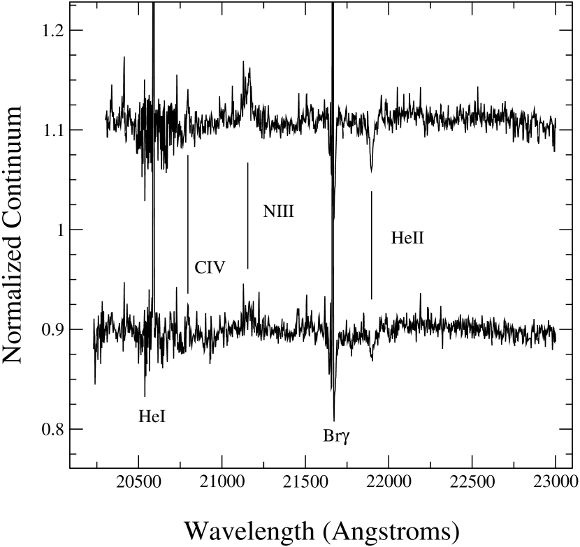
Figure 3: Spectra of O–type stars, “m” and “n,” from the first NIFS pointing; see Figure 1. Lines of C IV, He II, and N III identify these sources as mid or earlyO–type; see text. The spectra have been arbitrarily restricted in wavelength to show the weak stellar features. The spectral resolution is $R(\lambda/\Delta\lambda)=5160$. These spectra were normalized by a low order fit to the continuum after division by an A0 V type standard.

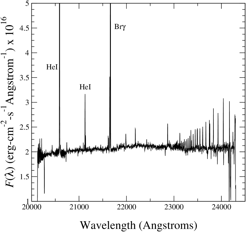
Figure 4: Combined spectrum of stars with nebular features, but no hot star photospheric features: “l”, from the first NIFS pointing and “g”, “h”, “i” from the second; see Figures 1 and 2. The spectral resolution is $R(\lambda/\Delta\lambda)=5160$. These spectra were normalized by an A0 V type standard and multiplied by a black body spectrum corresponding to $T_{\rm eff}=9000$K. The flux scale was set by assigning the flux at 2.12 $\mu$m according to the magnitudes given by Feldt et al. (1998) and a flux zero point at 2.12 $\mu$m of 4.75 $\times$10^-11 erg s^-1-cm^-2-$\mu$m^-1. Typical nebular lines of H and He are shown; other emission lines are described in the text and Figure 6.

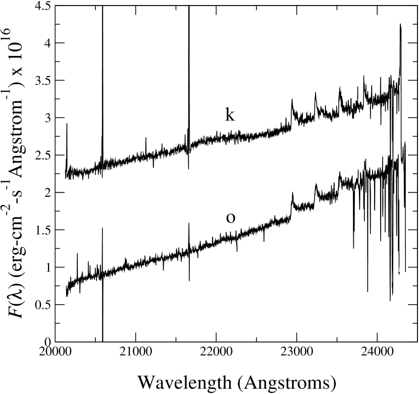
Figure 5: Spectra of CO emission stars,o, from the first NIFS pointing and k from the second; see Figures 1 and 2. The spectral resolution is $R(\lambda/\Delta\lambda)=5160$. These spectra were normalized by an A0 V type standard and multiplied by a black body spectrum corresponding to $T_{\rm eff}=9000$K.

Point source spectra are shown in Figures 3–5. Feldt et al. (1998) sources “m” and “n” exhibit photospheric features of mid–early O–type stars (Hanson et al., 1996). Though the telluric correction is relatively poor near 20600 Å, there appears to be weak C IV emission at 20796 Å and perhaps at 20842 Å in both sources (vacuum line positions from Ralchenko et al., 2007). The former line is stronger, as is typical (Hanson et al., 1996). The presence of C IV emission near 20800 Å together with the strong He II [absorption] and N III [emission] features indicates a spectral type earlier than about kO6 and later than about kO4. Sources “k” and “o” have CO overtone emission starting with the 2–0 rotational–vibrational bandhead at 22935 Å. These sources do not show obvious photospheric features. There is a suggestion of weak and broad absorption at the postion of Br$\gamma$ in the spectrum of source “k;” however, it is not possible to claim an unambiguous detection due to the strong nebular emission seen toward source “k” and the (imperfect) correction of Br$\gamma$ absorption in the telluric standard. Apart from CO bandhead emission, sources “k” and ”o” exhibit strong continuum emission and overlying, compact, nebular emission.

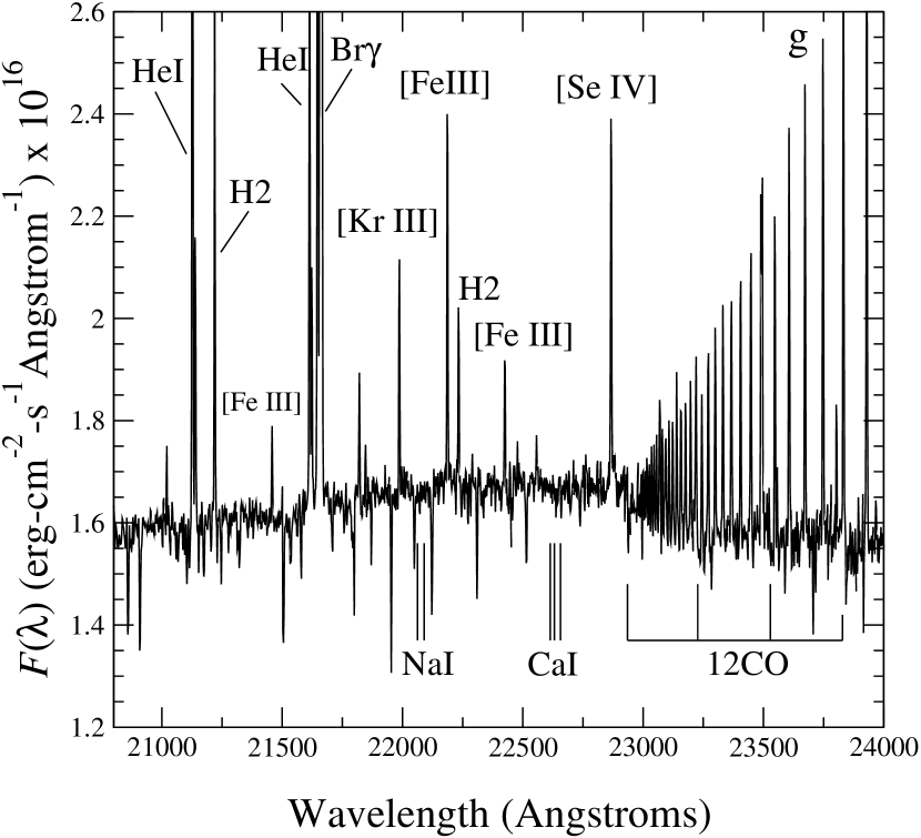
Figure 6: Same as Figure 4, but for source “g” alone and zoomed around the region of the CO first overtone bandhead at 22935 Å. There is an absorption component to the flux of source “g” due to young, lower mass star(s) in the ultra–compact H II region; see text. The positions of cool–star features due to NaI and CaI are indicated, but not confidently detected. The rich H I Pfund series is seen to the red side of 23000 Å. Other lines are also indicated (see text and Figure 8).

Sources “h”, “i”, and ”l” show only nebular features superimposed upon a red continuum. Source “g” exhibits a strong nebular spectrum, but upon close inspection, there appear to be “cool–star” absorption features superimposed upon the spectrum as well. Figure 6 shows the region of source “g” around the region of the CO 2–0 rotational–vibrational bandhead at 22935 Å.

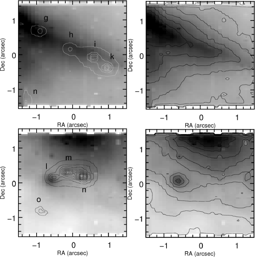
Figure 7: Br$\gamma$ line maps for pointing 1 (bottom row) and pointing 2 (top row). The continuum contours for a band at 21700 Å are overlaid on the left panels while the Brg$\gamma$ contours themselves are overlaid on the right. There is a compact Br$\gamma$ source in the continuum subtracted map for pointing 1 that appears to be associated with source “l”. The Br$\gamma$ contour levels (per 0.05$\times$0.05 arc second² pixel) are spaced by 1.1$\times$10^-17 erg cm^-2–s^-1 and 2.4$\times$10^-17 erg cm^-2–s^-1 in pointing 1 and 2, respectively. The peak contour level is 10 times the contour spacing in each pointing.

There are strong nebular emission lines throughout the three arc second field of view in pointings 1 and 2. Br$\gamma$ (21661 Å) and He I (20587 Å and 21127 Å) lines are strong as expected for an H II region with embedded hot stars. Figure 7 shows the distribution of ionized gas in each pointing along with an overlay of the contours of the continuum emission. The continuum band is centered near 21700 Å and it highlights the positions of the point sources relative to the ionized gas. A “point source” appears in the continuum–subtracted Br$\gamma$ map for pointing 1 that is near to, but not quite centered on, the position of source “l”. The ionized gas appears to form a sharp ridge in pointing two centered on the line of (presumably) embedded point sources, though the point sources appear systematically offset to the south as the ridge is traversed from east to west.

The peak Br$\gamma$ fluxes in each pointing are consistent with the narrow–band map presented by Feldt et al. (1998). The ratio of He I (21127 Å) to Br$\gamma$ is roughly uniform over both pointings and equal to about 0.035 $\pm$ 0.003 (not corrected for reddening).

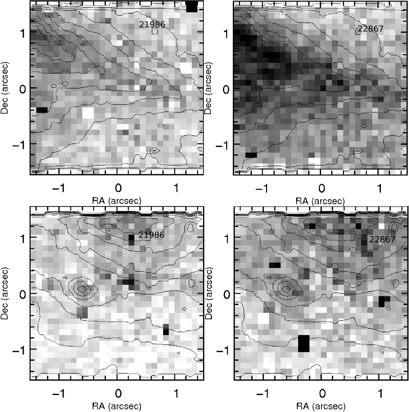
Figure 8: Line maps for pointing 1 (bottom row) and pointing 2 (top row) for emission centered near 21986 Å and 22867 Å. Br$\gamma$ contours themselves are overlaid on each panel. To improve signal to noise, these maps have been block averaged to 0.1^′′ by 0.1^′′ pixels (i.e. 2 by 2 binning).

Two lines present in the data cubes have been identified previously in planetary nebulae (PNe) spectra. These are the lines at 21986 Å and 22867 Å that were attributed to [Kr III] and [Se IV], respectively, in spectra of PNe by Dinerstein (2001). Figure 8 shows the gray–scale maps for both of these lines in each pointing (pointing 1, bottom; pointing 2, top). Each map is overlaid with the Br$\gamma$ contour, and it appears that the 21986 Å and 22867 Å lines trace the ionized gas region. All the lines detected are identified in Table 1. The line intensities with respect to Br$\gamma$ are similar in both pointings and all lines in the table were detected in both pointings.

5 Discussion

Feldt et al. (1998) used adaptive optics imaging at near–infrared wavelengths ($H$, and $K^{\prime}$ in conjunction with lower angular resolution radio and mid–infrared images to describe the evolutionary state of the UCH II region and its massive stars. Though their 4–m telescope data were still of insufficient resolution to make accurate photometric measurements of the bright trio of sources “l”, “m”, and “n”, they speculated that these sources were the more massive ionizing objects embedded in G45.45$+$0.06 and had formed first, triggering a second star formation event along the ridge of ionizing emission that gives this UCH II its original cometary designation (Wood & Churchwell, 1989). Our NIFS spectra of sources “m” and “n” confirm the first part of this scenario, at least. The two sources are hot, massive stars as identified by their photospheric features (Figure 3). G45.45$+$0.06 is thus one of only a few UCH II regions with spectroscopically confirmed central ionizing sources of the hottest spectral types (Watson & Hanson, 1997; Hanson et al., 2002; Bik et al., 2005), though identification of central stars in UCH II regions of mid O, late O, and early B types is now relatively common (Bik et al., 2005).

Along with the O–type stars, we have detected CO bandhead emission in sources “o” and “k”. This feature has been associated with massive young stellar objects (Bik & Thi, 2004; Blum et al., 2004; Bik et al., 2006). The brightness of source “k” ($K^{\prime}=$ 14.1; see Feldt et al., 1998) suggests it might be a hot star if its $H-Ks$ color were the result of reddening only. However, candidate massive stars with CO emission typically have strong excess emission due to reprocessing of the central star radiation by the circumstellar disk and/or envelope. It is more likely that the CO emission sources we observe in G45.45$+$0.06 are somewhat lower mass objects than the identified O–type stars and have not yet dispersed their natal cocoons as in W31 (Blum et al., 2001). See Blum et al. (2004) for an extended discussion of the near–infrared excess emission observed around young hot stars with CO emission.

The location of the CO emission sources and the apparently embedded sources “g”, “h”, and “i” outside the central “cluster” of O stars is consistent with a picture as described by Feldt et al. (1998) in which the O stars have triggered further star formation. However, as mentioned above, such embedded objects usually appear bright at $K$ due to strong excess emission (see the discussion in Blum et al., 2004), perhaps due to an accretion disk. The expected $K$ excess for objects with reprocessing disks can be quite large (2–4 mag) with a corresponding reduction in the resulting mass/luminosity (Hillenbrand et al., 1992). The disk (or envelope) dissipation time is longer for lower masses, so the issue of which stars formed when is unresolved. The strongest argument for triggered star formation remains the morphology of the sources embedded in the UCH II region. The source “g” appears to be the most heavily embedded source and the ionized gas systematically becomes separated from the point sources along the NE–SW ridge of emission as one moves toward source “k” to the SW (see Figure 7). The impression is that the hot stars “m” and “n” to the SE are ionizing this ridge and that if they are responsible for triggering the star formation events associated with the embedded sources, then perhaps source “k” formed first and has evolved slightly as the ionization front moves outward. Alternately, the lower mass stars have formed at the same time, but around the central high mass stars.

The UCH II region is powered by more than one massive star, and there are a number of lower mass hot (presumably B–type) stars as indicated by the NIFS spectroscopy. The exciting “star” of this UCH II region is, in fact, a cluster, as pointed out by Feldt et al. (1998); the NIFS data now provide a more quantitative description of the stellar content. This includes lower mass stars: Figure 6 suggests we have detected a cool–star component. The region of the spectrum near and beyond 23000 Å shows what appears to be bandhead absorption due to the CO molecule. The signal is strongest in the aperture around source “g” and it is not clear if source “g” itself is responsible for all the absorption or if there are one or more cooler stars very close to an otherwise more massive star. The strong Pfund series emission complicates the situation and is also contributing to the appearance of a lower “continuum” beyond 23000 Å (see Kraus et al., 2000). Nevertheless, a strong feature appears at the wavelength of the CO feature which does not have the smooth character expected for the psuedo continuum produced only by Pfund series lines running together.

Apertures with no obvious point source do not convincingly show a CO absorption signal, though any such signal should be weak. Meyer & Greissl (2005) made predictions of the integrated light signal from low–mass pre–main sequence (PMS) stars in massive clusters of $\sim$ Myr age. For lower resolution spectra ($R\equiv$ $\Delta\lambda/\lambda=$ 1000), they find CO bandhead absorption strengths of about one percent in integrated light. Our spectrum at higher resolution shows an absorption strength at 22935 Å of about five percent. Atomic features are also weak in the Meyer & Greissl (2005) spectra ($\mathrel{\hbox{\hbox to0.0pt{\hbox{\lower 4.0pt\hbox{$\sim$}}\hss}\hbox{$<$}}}$1 $\%$) and consistent with non–detections in our spectra (that have S/N $\sim$ 50). The low–mass signal depends on the amount of nebular emission (which degrades it) and age (younger PMS stars are brighter and have stronger features). The fact that we appear to detect low–mass stars in G45.45$+$0.06 suggests the cluster is quite young. Future work on modeling the low–mass component in UCH II regions might provide more quantitative age information than has been available to date for the associated massive stars. Precise ages are key to understanding disk dissipation and triggering time scales as mentioned above.

5.1 $T_{\rm eff}$ of the O–type stars

The spectral type assignment made in § 3 for sources “m” and “n” is accurate to a few sub–types. The infrared spectral type may be associated with optical types and an effective temperature determined for the stars. Previous estimates of the temperature vs. spectral type (Vacca et al., 1996) would give $T_{\rm eff}$ $\approx$ 44000 K to 48000 K (by association with the optical spectral types). Recent work using line–blanketed atmospheres (Martins et al., 2005) has resulted in the effective–temperature scale “cooling” so that these optical spectral types would give lower effective temperatures: $T_{\rm eff}$ $\approx$ 39000 K to 43000 K, a significant change. Repolust et al. (2005) used line blanketed models to derive O star effective temperatures directly from near–infrared and optical spectra. It is found that the effective temperatures are generally in good agreement for derivations using near–infrared and optical spectra. Repolust et al. (2005) report $T_{\rm eff}$ $=$ 42000 and 45000 derived from fits to near–infrared spectra for an O4V star and O3V star, respectively. We thus expect the effective temperature for sources “m” and “n” to lie within the range given by Martins et al. (2005), i.e. about $T_{\rm eff}$ $=$ 41000 K $\pm$ 2500 K.

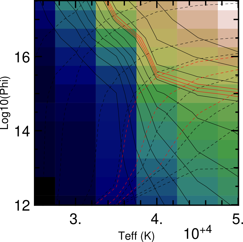
Figure 9: The ratio of HeI 21126 to Br$\gamma$ (reddening free or intrinsic) for a grid of Cloudy ionization models is shown in color and with solid contours. The red solid contour is the observed value (0.037, corrected for $A_{K}=$ 2 and shown with two other contours corresponding to $\pm$ 0.5 mag of extinction). The dashed contours are the results from the same models for the ratio of Br$\gamma$ (again corrected for 2 $\pm$ 0.5 mag of extinction) to the total dust emission. The observed dust emission is taken from the spectral energy distribution presented by Feldt et al. (1998); see text. The intersection of the observed values for the two contour families is consistent with the expectation of the $T_{\rm eff}$ from the infrared spectral types of sources “m” and “n”.

The observed emission–line and dust properties of G45.45$+$0.06 can also be used to constrain the effective temperature of exciting source(s). We used Cloudy ionization models to predict the ratio of HeI (21126 Å) to Br$\gamma$ and the total far infrared flux for a range of $T_{\rm eff}$ and ionizing photon flux. The results are shown in Figure 9. The simulations follow the procedure described by Blum & Damineli (1999) but use HeI 21126 Å instead of HeI 20587 Å. The simulations used the Castelli & Kurucz (2004) log($g$) $=$ 5 models, an electron density of 10⁴, and “$\_$ism” abundances and were run until the zone temperature was 100 K to better simulate an UCH II region. The density is constrained by the ratio of [Fe III] lines (21457 Å/21284 Å$=$ 0.4 corrected for $A_{K}$ $=$ 2; see Table 1 and Lutz et al. 1993).

The He I to Br$\gamma$ ratio (0.034; see Table 1) is uniform across the two pointings and as shown by Hanson et al. (2002, see also Benjamin et al. 1999) suggests an exciting star whose $T_{\rm eff}$ is greater than about 40000 K. A correction of 1.08 was used to account for the differential reddening expected for $A_{K}=$ 2 mag (Feldt et al., 1998). Figure 9 shows in color and solid contours the predicted ratio of He I to Br$\gamma$ for a grid of models whose axes are the log of incident ionizing flux and the central source effective temperature. The observed line ratio (0.037) is shown in a solid red contour (corrected for reddening) along with solid contours corresponding to $\pm$ 0.5 mag of extinction. The ratio increases monotonically at constant ionizing photon flux as the $T_{\rm eff}$ increases. The exciting source $T_{\rm eff}$ shows a range of values for the observed contour depending on the ionizing photon flux.

This degeneracy may be broken, in principle, by plotting the observed ratio of Br$\gamma$ to the total dust emission. In practice, this comparison is difficult due to the different aperture sizes used to map these two quantities. To make an approximate comparison, consider the spectral energy distribution (SED) given by Feldt et al. (1998) using their observations at near–infrared and mid infrared wavelengths coupled with IRAS data points. The flux density peaks near 100 $\mu$m. Integrating this SED and dividing by the Feldt et al. 11^′′ diameter aperture, we find a dust surface brightness of 1.3$\times$10^-9 erg cm^-2–s^-1 per square arc second where we have reduced the IRAS flux by a factor of three so that the IRAS points join smoothly with the Feldt et al. (1998) mid–infrared data (the difference is apparently due to the different aperture sizes as noted by Feldt et al.). From Figure 7, we take a typical value of the Br$\gamma$ flux to be 3.5$\times$10^-14 erg cm^-2–s^-1 per square arc second. The ratio of Br$\gamma$ to dust emission from the Cloudy grid is plotted as dashed contours in Figure 9. The observed ratio (corrected for $A_{K}=$ 2.0 mag) is plotted as a red dashed contour with two other red contours corresponding to the Br$\gamma$ value for 1.5 mag and 2.5 mag $A_{K}$, respectively. The intersection of the red solid and red dashed contours is consistent with an effective temperature in the same range we expect from the spectral types of sources “m” and “n” and a best value at the hot end of the range of temperatures allowed by the spectral type.

5.2 The Distance to G45.45$+$0.06

The NIFS photometry for sources “m” and “n” is too uncertain to estimate a reliable distance. In addition, we have no $H$ magnitudes from which to derive precise extinction measurements. But a rough consistency check can be made using the extinction map generated by Feldt et al. (1998) which gives $A_{K}$ $\approx$ 2 mag. Blum et al. (2000) provide $M_{K}$ values for ZAMS stars as a function of spectral type. This relation might change when accounting for the new effective temperature scale described above, but this change actually changes the $M_{V}$ of dwarf O stars very little at the high mass end ($\mathrel{\hbox{\hbox to0.0pt{\hbox{\lower 4.0pt\hbox{$\sim$}}\hss}\hbox{$<$}}}$0.1 mag, Martins et al., 2005), so the $M_{K}$ should be approximately correct. Using the derived magnitudes for “m” and “n’, the extinction value quoted above, and $M_{K}$ from Blum et al. (2000) appropriate to an O3 star ($-$4.8), the distance to G45.45$+$0.06 would be about 10 kpc when averaging over the two sources. If the O5 $M_{K}$ were used instead, the distance would be 7 kpc. Feldt et al. (1998) adopt a value of 6.6 kpc based on radio measurements. Given the uncertainties in the photometry, extinction, and ZAMS $M_{K}$ scale, this result is roughly consistent with the Feldt et al. (1998) value.

5.3 High Excitation Emission Lines from $s$–process Elements

The two $s$–process lines ([Kr III] 21986 Å and [Se IV] 22867 Å) were identified by Dinerstein (2001) based on ionization potential and the close match between the observed wavelengths in PNe and those expected from the fine–structure energy levels arising in the two ions. Dinerstein (2001) built on the work of Geballe et al. (1991) who showed the (then) unidentified lines were not due to H₂ (the wavelengths did not match) and that the lines appeared only in intermediate excitation planetaries. Geballe et al. (1991) observed the compact H II region IRS2 in W51 along with the PNe and found no line emission at 21986 Å or 22867 Å in IRS2. From these observations, Geballe et al. (1991) deduced the ionization potential of the parent atom or ion must be in the range 30–40 eV and that the ionization potential for the ion itself should lie at about 40–60 eV. Dinerstein (2001) estimated the abundances of the two species from their observed line strengths and concluded they were in line with expectations if there were some modest enhancement due to $s$–processing in the PNe central stars coupled with third dredge up to the pre–planetary surface layers.

Of the 13 PNe observed by Geballe et al. (1991) few have effective temperatures similar to O–stars. Several are cooler, and the majority are much hotter (Kaler & Jacoby, 1991). The coolest (28000 K) does not exhibit the lines, but several with temperatures in the $\sim$ 60000–80000 K range do show the lines and with similar ratios to Br$\gamma$ as given in Table 1 (i.e., $\mathrel{\hbox{\hbox to0.0pt{\hbox{\lower 4.0pt\hbox{$\sim$}}\hss}\hbox{$<$}}}$few percent). Sterling et al. (2007$a$) have embarked on a large survey of PNe for which they are doing detailed photo–ionization modeling. They report results for a set of 10 PNe that they are using to calibrate the atomic data for Kr and Se that are somewhat uncertain. In any case, they have observed several cooler PNe (37000, 56000 K). Neither of these cool PNe exhibits both [Kr III] and [Se IV], but each exhibits one of the lines, and in similar ratio to Br$\gamma$ as found in this work for G45.45$+$0.06 (Table 1). The abundances of Kr and Se appear to be enhanced in many, but not all PNe with respect to the Solar value (see Sterling et al., 2007$b$, for preliminary results of the large PNe survey).

The presence of two relatively high–excitation lines ([Kr III] 21986 Å and [Se IV] 22867 Å) was unexpected given that these lines have been identified in PNe of fairly high excitation, and are not typical of H II regions. However, search of the literature shows that these “unidentified” lines have been detected in a number of H II regions even though the explicit association with [Kr III] and [Se IV] had not been made. Lumsden & Puxley (1996) suggested they may have detected both unidentified lines in their low resolution spectrum of G45.12$+$0.13, but could not confidently separate the 21986 Å line from H₂. Lumsden & Puxley (1996) derived an excitation temperature in G45.12$+$0.13 between 38000 K and 42000 K. Okumura et al. (2001) studied the same UCH II region, IRS2 in W51 as did Geballe et al. (1991), and detected the [Se IV] line. It appears the [Kr III] line is also present though again blended with H₂ 3–2 (S3) line (this is evident when comparing the “excess” level population at the energy corresponding to an upper level of 19086K; see their Figure 4 and Table 5). Better angular resolution may be the reason Okumura et al. (2001) were able to identify the line while Geballe et al. (1991) did not. Another possibility is differences in the detailed slit positioning in/around IRS2.

Aspin (1994) detected the lines in a spectrum of the object IRS 1 that is near the exciting source GGD27–IRS of both HH80 and HH81 (but otherwise not related). Aspin (1994) noted the possible association of the lines with those seen by Geballe et al. (1991). It is not clear what type of object might be exciting IRS 1 (see Yamashita et al., 1987; Aspin et al., 1991). The “unidentified” line at 21986 Å has also been detected in the extragalactic giant H II region NGC 5461. Puxley et al. (2000) note the H₂ 3–2 S(3) line is blended with a line they associate with the unidentified line cited by Geballe et al. (1991).

Hanson et al. (2002) presented $K-$band spectra for a sample of UCH II regions, but do not mention detection of either of these two lines. Their spectral coverage ran out near the 22867 Å line, but one of their spectra of a “typical” UCH II region (see their Figure 1) shows a line near 21986 Å that may be due to [Kr III]. Bik et al. (2005) also surveyed a number of UCH II regions, but their spectra do not cover the two line positions. Bik et al. (2006) investigated deeply embedded point sources in compact H II regions; their spectra do not show evidence of either line, but it is likely these sources are of lower effective temperature typical of early B–type and late O–type stars. Blum and collaborators (Blum et al., 1999, 2000, 2001; Figuerêdo et al., 2002, 2005) have surveyed giant H II regions using $K-$band spectroscopy, but they also do not report detections of these two lines; a number of their spectra also do not cover the line regions. The lack of sufficient wavelength coverage has been due to the trade off in instrumental spectral resolution. Surveys for massive stars usually tend to the blue end of the $K-$band to cover the O–type star diagnostic lines. Most of the investigations mentioned above have also concentrated on the point source spectroscopy of candidate massive stars and not the overall nebular spectrum of the regions and objects surveyed.

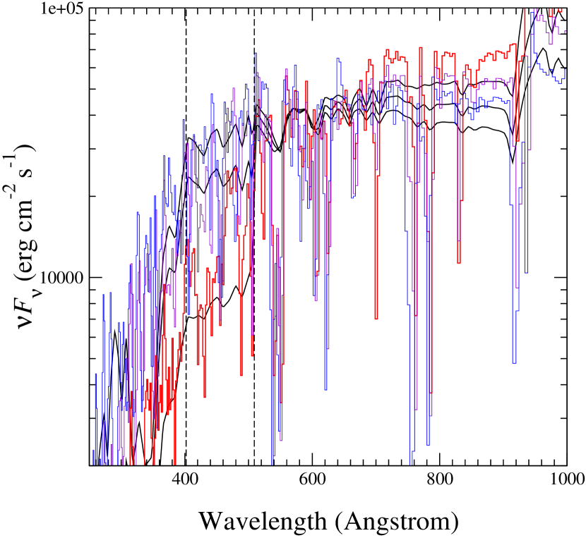
Figure 10: Kurucz model atmosphere (Castelli & Kurucz, 2004, black solid lines) and WMBASIC (Pauldrach et al., 2001, colored histograms) incident continua for 36000 K, 42000 K, and 46000 K hot stars. The vertical dashed lines correspond to the ionization potentials of Kr II and Se III. The higher $T_{\rm eff}$ models appear to have significant numbers of ionizing photons in the spectral regions required to produce Kr III and Se IV; see text. All spectra are normalized to the same total number of ionizing photons (log(Q) cm^-2 s^-1 $=$ 15). Both model sets show significant numbers of ionizing photons in the range required to produce Kr III and Se IV for the hotter stars. The cooler stars show a precipitous drop in ionizing photons.

The ionization potentials for Kr II and Se III are 24.4 eV and 30.8 eV, respectively (Dinerstein, 2001). This is well within the range of the ionizing continuum of the hotter O–type stars, particularly for Kr II. Figure 10 shows the ionizing continua of hot stars for a range of effective temperatures and two sets of models. Plane parallel, hydrostatic models are plotted (Castelli & Kurucz, 2004) along with line blanketed wind models (Pauldrach et al., 2001). Both show significant numbers of ionizing photons for the hotter stars and a rapid decrease in ionizing photons in the range appropriate to form Kr III and Se IV as the effective temperature falls. Wavelengths corresponding to the ionization potentials of Kr II and Se III are shown as vertical dashed lines.

While the presence of these two lines is not ubiquitous in H II region spectra, it seems that the hotter O stars, in dense UCH II regions, can produce these lines. The distribution of the emission within the UCH II follows the ionized gas as shown in the maps of Figure 7 and 8. Our unpublished NIFS data for the UCH II region G5.89$-$0.39 show strong emission at 21986 Å and possibly weaker emission at the [Se IV] position toward the center of the UCH II region. We were unable to identify the exciting source in this case, but the excitation as given by the HeI to Br$\gamma$ ratio and Br$\gamma$ to dust ratio appears similar to that for G45.45$+$0.06. A detailed analysis of the G5.89$-$0.39 data is in progress. Given the ionization potentials of the parent ions to the species responsible for these lines and the strong gradient in the ionizing continuum hardness of the O stars, we believe that these lines will only be produced in dense H II regions with the hottest ionizing stars.

6 Summary

NIFS 3-dimensional imaging spectroscopy is presented for two pointings toward the UCH II region G45.45$+$0.06. The central ionizing sources of G45.45$+$0.06 have been identified as massive O–type stars through comparison of their $K-$band spectra to template O star spectra. The Feldt et al. (1998) sources “m” and “n” are found to be of O spectral types earlier than about kO6. In addition, two other Feldt et al. (1998) sources, “k” and “o”, exhibit CO bandhead emission near 23000 Å indicating that they are massive young stellar objects. In analogy to other similar objects in other H II regions, these two massive young stellar objects likely have significant $K-$ band excesses and thus have central stars consistent with late O and early B stars. The remaining Feldt et al. (1998) sources in the NIFS fields (“l”, “g”, “h”, and “i”) show strong compact nebular emission and rising red continua suggesting that they too are massive young stellar objects.

The NIFS images reveal complex nebular structure and precise emission line maps. The morphology of the UCH II region suggests that the central hot stars have triggered star formation in the material to the north west as represented by point sources “g”, “h”, “i”, and “k” and also to the south in the form of source “o”. However, there is no way to precisely assign ages to these sources relative to the central ionizing stars that are presumably on, or near, the zero age main sequence. Modeling the weak signal from low–mass pre–main sequence stars may provide a much needed clock for high–mass starforming regions. A low–mass signal is present in the NIFS data for G45.45$+$0.06, though it is not clear if it is associated with one or a few low–mass objects. An alternate scenario is that the massive stars form in the cluster center and lower mass stars form around them at the same time.

Lines of doubly ionized Kr and triply ionized Se are detected in the NIFS spectra. Line maps show that these lines follow the ionized gas in the UCH II region as traced by Br$\gamma$ and HeI. The lines are not common in H II regions, but have been identified in planetary nebulae (PNe) where the central stars are typically much hotter. In fact, one or the other or both of the lines, while not previously identified with Kr III and Se IV, have been detected in a number of compact H II regions. The Kr III line, in particular, is blended with H₂ 3–2 S(3) at lower spectral resolution making its identification more difficult.

These are $s$–process lines that show enhanced abundances over the Solar value for some, but not all, PNe. We suggest that it may be only the H II regions excited by the hottest O stars and with high density that can produce these lines. If so, the lines may be a useful new diagnostic on the effective temperature of ionizing stars in H II regions. Much of the observational data in the literature are incomplete with respect to wavelength coverage for the detection of these lines in a wide range of H II regions, and the atomic parameters of the ions of Kr and Se are not yet well established, but progress is being made on both fronts.

We acknowledge the helpful comments of an anonymous referee. The plots and analysis in this article made use of the Yorick programing language. This article made use of the SIMBAD database at the CDS. The authors would like to thank Tom Geballe for initially pointing out the line identifications for Kr and Se and Dick Shaw for useful discussions regarding planetary nebulae.

Table 1: Emission Line Identifications and Ratios

Line Identification	Wavelength (Å)	Pointing 1 Ratio to Br$\gamma$	Pointing 2 Ratio to Br$\gamma$
HeI 1S–1P∘	20587	0.865 $\pm$ 0.0015	0.812 $\pm$ 0.0011
HeI 3P∘–3S	21126	0.035 $\pm$ 0.0003	0.034 $\pm$ 0.0002
HeI 1P∘–1S	21138	0.012 $\pm$ 0.0002	0.009 $\pm$ 0.0001
H2 v$=$1–0 S(1)	21218	0.015 $\pm$ 0.0002	0.015 $\pm$ 0.0001
$[$Fe III$]$ 3H–3G	21457	0.007 $\pm$ 0.0002	0.003 $\pm$ 0.0001
HeI 3D–3F∘	21614	0.022 $\pm$ 0.0002	0.020 $\pm$ 0.0001
HeI 1D–1F∘	21623	0.006 $\pm$ 0.0002	0.007 $\pm$ 0.0001
HeI	21646	0.044 $\pm$ 0.0003	0.049 $\pm$ 0.0002
Br$\gamma$ (HI 7–4)	21661	1.000 $\pm$ 0.0017	1.000 $\pm$ 0.0012
HeI?	21820	0.005 $\pm$ 0.0002	0.004 $\pm$ 0.0001
HeI 1P∘–1D	21846	0.006 $\pm$ 0.0002	0.003 $\pm$ 0.0001
$[$Kr III$]$ 3P1–3P2	21987	0.008 $\pm$ 0.0002	0.006 $\pm$ 0.0001
$[$Fe III$]$ 3H–3G	22184	0.018 $\pm$ 0.0002	0.017 $\pm$ 0.0001
H2 v$=$1–0 S(0)	22233	0.006 $\pm$ 0.0002	0.005 $\pm$ 0.0001
$[$Fe III$]$ 3H–3G	22427	0.006 $\pm$ 0.0002	0.006 $\pm$ 0.0001
H2 v$=$ 2–1 S(1)	22477	0.004 $\pm$ 0.0002	0.001 $\pm$ 0.0001
$[$Se IV$]$ 2P3/2–2P1/2	22867	0.013 $\pm$ 0.0002	0.012 $\pm$ 0.0001

References

- Aspin et al. (1991) Aspin, C., Casali, M. M., Geballe, T. R., & McCaughrean, M. J. 1991, A&A, 252, 299
- Aspin (1994) Aspin, C. 1994, A&A, 281, L29
- Benjamin et al. (1999) Benjamin, R. A., Skillman, E. D., & Smits, D. P. 1999, ApJ, 514, 307
- Bik & Thi (2004) Bik, A., & Thi, W. F. 2004, A&A, 427, L13
- Bik et al. (2005) Bik, A., Kaper, L., Hanson, M. M., & Smits, M. 2005, A&A, 440, 121
- Bik et al. (2006) Bik, A., Kaper, L., & Waters, L. B. F. M. 2006, A&A, 455, 561
- Black & van Dishoeck (1987) Black, J. H., & van Dishoeck, E. F. 1987, ApJ, 322, 412
- Blum & Damineli (1999) Blum, R. D., & Damineli, A. 1999, ApJ, 512, 237
- Blum et al. (1999) Blum, R. D., Damineli, A., & Conti, P. S. 1999, AJ, 117, 1392
- Blum et al. (2000) Blum, R. D., Conti, P. S., & Damineli, A. 2000, AJ, 119, 1860
- Blum et al. (2001) Blum, R. D., Damineli, A., & Conti, P. S. 2001, AJ, 121, 3149
- Blum et al. (2004) Blum, R. D., Barbosa, C. L., Damineli, A., Conti, P. S., & Ridgway, S. 2004, ApJ, 617, 1167
- Castelli & Kurucz (2004) Castelli, F., & Kurucz, R. L. 2004, ArXiv Astrophysics e-prints, arXiv:astro-ph/0405087
- Churchwell (2002) Churchwell, E. 2002, ARA&A, 40, 27
- Dinerstein (2001) Dinerstein, H. L. 2001, ApJ, 550, L223
- Drake & Martin (1998) Drake, G. W. F. & Martin, W. C. 1998, Can, J. Phys., 76, 679
- Feldt et al. (1998) Feldt, M., Stecklum, B., Henning, T., Hayward, T. L., Lehmann, T., & Klein, R. 1998, A&A, 339, 759
- Ferland et al. (1998) Ferland, G. J., Korista, K. T., Verner, D. A., Ferguson, J. W., Kingdon, J. B., & Verner, E. M. 1998, PASP, 110, 761
- Figuerêdo et al. (2002) Figuerêdo, E., Blum, R. D., Damineli, A., & Conti, P. S. 2002, AJ, 124, 2739
- Figuerêdo et al. (2005) Figuerêdo, E., Blum, R. D., Damineli, A., & Conti, P. S. 2005, AJ, 129, 1523
- Geballe et al. (1991) Geballe, T. R., Burton, M. G., & Isaacman, R. 1991, MNRAS, 253, 75
- Hanson et al. (1996) Hanson, M. M., Conti, P. S., & Rieke, M. J. 1996, ApJS, 107, 281
- Hanson et al. (2002) Hanson, M. M., Luhman, K. L., & Rieke, G. H. 2002, ApJS, 138, 35
- Hillenbrand et al. (1992) Hillenbrand, L. A., Strom, S. E., Vrba, F. J., & Keene, J. 1992, ApJ, 397, 613
- Kaler & Jacoby (1991) Kaler, J. B., & Jacoby, G. H. 1991, ApJ, 372, 215
- Kraus et al. (2000) Kraus, M., Krügel, E., Thum, C., & Geballe, T. R. 2000, A&A, 362, 158
- Lumsden & Puxley (1996) Lumsden, S. L., & Puxley, P. J. 1996, MNRAS, 281, 493
- Lutz et al. (1993) Lutz, D., Krabbe, A., & Genzel, R. 1993, ApJ, 418, 244
- Martins et al. (2005) Martins, F., Schaerer, D., & Hillier, D. J. 2005, A&A, 436, 1049
- McGregor et al. (2003) McGregor, P. J., Hart, J., Conroy, P. G., Pfitzner, M. L., Bloxham, G. J., Jones, D. J., Downing, M. D., Dawson, M., Young, P., Jarnyk, M., & van Harmelen, J. 2003, SPIE, 4841, 1581.
- Messineo et al. (2007) Messineo, M., Petr-Gotzens, M. G., Schuller, F., Menten, K. M., Habing, H. J., Kissler-Patig, M., Modigliani, A., & Reunanen, J. 2007, A&A, 472, 471
- Meyer & Greissl (2005) Meyer, M. R., & Greissl, J. 2005, ApJ, 630, L177
- Okumura et al. (2001) Okumura, S.-i., Mori, A., Watanabe, E., Nishihara, E., & Yamashita, T. 2001, AJ, 121, 2089
- Ralchenko et al. (2007) Ralchenko, Yu., Jou, F.-C., Kelleher, D.E., Kramida, A.E., Musgrove, A., Reader, J., Wiese, W.L., & Olsen, K. (2007). NIST Atomic Spectra Database (version 3.1.2), [Online]. Available: http://physics.nist.gov/asd3 [2007, August 24]. National Institute of Standards and Technology, Gaithersburg, MD.
- Repolust et al. (2005) Repolust, T., Puls, J., Hanson, M. M., Kudritzki, R.-P., & Mokiem, M. R. 2005, A&A, 440, 261
- Pauldrach et al. (2001) Pauldrach, A. W. A., Hoffmann, T. L., & Lennon, M. 2001, A&A, 375, 161
- Puxley et al. (2000) Puxley, P. J., Ramsay Howat, S. K., & Mountain, C. M. 2000, ApJ, 529, 224
- Sterling et al. (2007) Sterling, N. C., Dinerstein, H. L., & Kallman, T. R. 2007, ApJS, 169, 37
- Sterling et al. (2007) Sterling, N. C., Dinerstein, H. L., & Kallman, T. R. 2007, ArXiv e-prints, 708, arXiv:0708.1323
- Vacca et al. (1996) Vacca, W. D., Garmany, C. D., & Shull, J. M. 1996, ApJ, 460, 914
- Watson & Hanson (1997) Watson, A. M., & Hanson, M. M. 1997, ApJ, 490, L165
- Wood & Churchwell (1989) Wood, D. O. S., & Churchwell, E. 1989, ApJS, 69, 831
- Yamashita et al. (1987) Yamashita, T., Sato, S., Nagata, T., Suzuki, H., Hough, J. H., McLean, I. S., Garden, R., & Gatley, I. 1987, A&A, 177, 258