Universal Properties of Ferroelectric Domains

Abstract

Basing on Ginzburg-Landau approach we generalize the Kittel theory and derive the interpolation formula for the temperature evolution of a multi-domain polarization profile $\mathbf{P}(x,z)$. We resolve the long-standing problem of the near-surface polarization behavior in ferroelectric domains and demonstrate the polarization vanishing instead of usually assumed fractal domain branching. We propose an effective scaling approach to compare the properties of different domain-containing ferroelectric plates and films.

Design of ferroelectric devices necessitates taking into account such finite size effects as the formation of polarization-induced surface charges that, in turn, produce the energy consuming electrostatic depolarizing fields (see Ref.2005_Dawber for review). As a result, regular periodic structures of $180^{0}$ domains that alternates the surface charge distribution, firstly proposed by Landau and Lifshitz1935_Landau ; Landau8 and by Kittel1946_Kittel for ferromagnetic systems, can be formed in uniaxial easy-axis (natural or stress-induced) ferroelectric plates or films as an effective mechanism to confine the depolarization field to the near-surface layer and reduce its energy (Fig.1a). The energy balance between the field-penetration depth ($\sim$ domain width $d$) and domain wall (DW) concentration ($\sim d^{-1}$) leads to the famous square-root Kittel dependence of $d$ on the film thickness $2a_{f}$ 1946_Kittel ; 2000_Bratkovsky ; Guerville ; 2007Catalan :

$$d=\sqrt{\gamma\,(\epsilon_{\perp}/\epsilon_{\parallel})^{1/2}\,(2a_{f}\,\xi_{0x})}\,,\quad\gamma={\frac{2\sqrt{2}\pi^{3}}{21\zeta(3)}}\simeq 3.53,$$ (1)

where $\epsilon_{\parallel}$ and $\epsilon_{\perp}$ are the longitudinal and transversal dielectric constants and $\xi_{0x}$ is the transverse coherence length (roughly equal to the DW thickness).

a)        b)
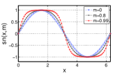
c) .

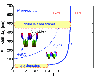
Figure 1: (a)Multi-domain texture of ferroelectric polarization in uniaxial ferroelectric film, sandwiched by two paraelectric (dead)-layers. The emerging depolarization electric field is provided by alternating polarization-induced surface charges and confined in the near-surface layer of thickness, comparable with domain width $d$. (b) Elliptical functions $y=\mathrm{sn}(x,m)$ for different parameters $m$ that we use to model the domain profile at different $t$. (c) Phase diagram of domain states as function of sample thickness $2a_{f}$ and reduced critical temperature $t=T/T_{c0}-1$. Polarization profiles of hard and soft domains were obtained by numerical solution of equations (6)-(9). We assume that $\varkappa_{\parallel}\simeq 500$, $\varepsilon_{\perp}\simeq 100$, $\varepsilon_{p}\ll\varepsilon_{\perp},\varkappa_{\parallel}$, $\xi_{0x}\simeq 1nm$ and $a_{p}\simeq 30nm$.

Consider the standard geometry 2000_Bratkovsky when the uniaxial ferroelectric film is sandwiched by electroded paraelectric passive layers of width $a_{p}$ and permittivity $\varepsilon_{p}$. The multi-domain state should exist in certain intervals of film thickness $2a_{f}$ as shown in phase diagram in Fig.1c and defined by the condition that delineates the applicability of Eq.(1) and of our further consideration:

$$\xi_{0x}<d(2a_{f})<a_{p}$$ (2)

the dependence $d(2a_{f})$ being given by (1). We also assume the most realistic case $\varepsilon_{p}\ll\varepsilon_{{}_{\perp}}<\varepsilon_{{}_{\parallel}}$ that gives $d\ll a_{f}$. At this stage the properties of domain structure do not depend on $a_{p}$, $\varepsilon_{p}$ and electrodes. For thicker films, when $d(2a_{f})$ approaches to $a_{p}$ the emergent depolarizing field interacts with screening electrodes, Eq.(1) is not valid anymore, $d$ growth exponentially with $a_{p}^{-2}$ 2000_Bratkovsky and domains practically emerge from the sample. However in free standing electrodless sample ($a_{p}\rightarrow\infty$) Kittel domains can exist in a wider interval of $2a_{f}$ unless another restricting mechanism of the internal free charges screening does not came into the play. For thinner films we are turning to the region of little-studied atomic-size (microscopic) domains Bratkovsky2006 .

While domain structures should play a crucial role in the properties of thin ferroelectric films, only a few theoretical analytical studies of their temperature dependence have been performed. In particularly the mostly used Kittel approach Landau8 ; 1946_Kittel ; 2000_Bratkovsky in which the domain texture is considered as a set of up- and down- oriented (hard) domains, having a flat polarization profile $\mathbf{P}(x,z)=\pm P_{0}$, DW are supposed to be infinitely thin and boundary effects on the ferroelectric-paraelectric interface are neglected, is valid only far below the transition temperature $T_{c}$. Although the more general consideration, proposed by Chensky and Tarasenko (CT)1982_Chensky (see also Guerville ; 2004_Stephanovich ) is based on Ginzburg-Landau equations coupled with electrostatic equations is valid in the whole temperature interval, only the solution close to $T_{c}$ was found.

It is the objective of the present communication to establish the approach that permits to model the temperature evolution of domain structure. Basing on CT equations we derive the analytical expression (19) for domain polarization profile that is valid in the whole temperature interval and includes the Kittel (at low $T$) and CT (at $T=T_{c}$) solutions as particular cases. Then, we deduce universal scaling relations between parameters of the multi-domain state that should be useful in treatment of experimental data. Our approach is complimentary to the frequently used first-principia simulations (see e.g. Bo-Kuai_2006 ), that reproduce the domain structure but give no general vision and parameter dependence of the results.

Deducing the CT equations we are basing on the Euler-Lagrange variational formalism, that permits also to obtain the correct boundary conditions as variation of surface terms. The generating energy functional is written as Landau8 :

$$F=\int\widetilde{\Phi}(\mathbf{P},\mathbf{E})dxdz,\quad\widetilde{\Phi}(\mathbf{P},\mathbf{E})=\widetilde{\Phi}(\mathbf{P},0)-\mathbf{EP}-\frac{1}{8\pi}\mathbf{E}^{2}$$ (3)

where $\mathbf{E}=(E_{x},E_{z})$, $\mathbf{P}=(P_{x},P_{z})$ and the field-independent part

$$\widetilde{\Phi}(\mathbf{P},0)=\frac{4\pi}{\varepsilon_{\perp}}\frac{1}{2}P_{x}^{2}+\frac{4\pi}{\varepsilon_{i\parallel}}\frac{1}{2}P_{zi}^{2}+\frac{4\pi}{\varkappa_{\parallel}}f(P)$$ (4)

includes the transversal $P_{x}$, and non-polar longitudinal $P_{zi}$ noncritical contributions ($\varepsilon_{\perp}$,$\varepsilon_{i\parallel}\gg 1$). The nonlinear Ginzburg-Landau energy depends on the spontaneous $z$-oriented polarization $P$ (assuming that $P_{z}=P_{zi}+P$) and is written as:

$$f(P)=\frac{t}{2}P^{2}+\frac{1}{4}P_{0}^{-2}P^{4}+\frac{\xi_{0x}^{2}}{2}\left(\partial_{x}P\right)^{2}+\frac{\xi_{0z}^{2}}{2}\left(\partial_{z}P\right)^{2}$$ (5)

where the reduced temperature $t$ is expressed via the bulk critical temperature as: $t=T/T_{c0}-1$, parameter $\varkappa_{\parallel}$ is expressed via paraelectric Curie constant $C$ and via longitudinal zero-temperature permittivity $\varepsilon_{\parallel}$ in (1) as: $\varkappa_{\parallel}=C/T_{c0}\simeq 2\varepsilon_{\parallel}$ , and coefficient $P_{0}$ is roughly equal to the saturated bulk polarization at $T\ll T_{c}$

The variation of (3) with respect to $P$ and the electrostatic potential $\varphi$ ($\mathbf{E}=-\nabla\varphi$) and excluding of the non-essential variables $P_{x}$ and $P_{zi}$ gives the system of required equations that describe the ferroelectric transition taking into account the depolarizing field:

$$(t-\,\xi_{0x}^{2}\partial_{x}^{2}-\xi_{0z}^{2}\partial_{z}^{2})P+(P/P_{0})^{2}P=-\frac{\varkappa_{\parallel}}{4\pi}\partial_{z}\varphi,$$ (6)

$$(\varepsilon_{i\parallel}\partial_{z}^{2}+\varepsilon_{\perp}\partial_{x}^{2})\varphi=4\pi\partial_{z}P.$$

These equations should be completed by the Poisson equation for paraelectric media in which ferroelectric film is embedded:

$$(\partial_{z}^{2}+\partial_{x}^{2})\varphi^{(p)}=0,$$ (7)

and by boundary conditions at the Para-Ferro interface

$$\varepsilon_{i\parallel}\partial_{z}\varphi-\varepsilon_{p}\partial_{z}\varphi^{(p)}=4\pi P,\quad\varphi=\varphi^{(p)},\quad\partial_{z}P=0.$$ (8)

that are also obtained as result of variation of (3) remark . Periodic conditions

$$P(x,z)=P(x+2d,z)\quad\varphi(x,z)=\varphi(x+2d,z)$$ (9)

with variational parameter $d$ are imposed to describe the periodicity of domain structure.

A simplification can be achieved if present the initial functional (3) using the dimensionless (prime) variables:

$$z = a_{f}\,z^{\prime},\quad x=\tau^{-1/2}\xi_{0x}\,x^{\prime},\quad t=\tau\,t^{\prime},$$ (10)

$$P = \tau^{1/2}P_{0}\,P^{\prime},\quad\varphi=\frac{1}{\varkappa_{\parallel}}\,\tau^{3/2}\,a_{f}P_{0}\,\varphi^{\prime},$$

$$F = \frac{a_{f}\,\xi_{0x}}{\varkappa_{\parallel}}\tau^{3/2}\,P_{0}{}^{2}\,F^{\prime}\,\,\,\,\,\,\,\,\,\,$$

with

$$\tau=\left(\frac{\varkappa_{\parallel}}{\varepsilon_{\perp}}\right)^{\frac{1}{2}}\frac{\xi_{0x}}{a_{f}}\ll 1$$ (11)

in truncated form,

$$F^{\prime} = \int[4\pi\left(\frac{1}{2}t^{\prime}P^{\prime 2}+\frac{1}{4}P^{\prime 4}+\frac{1}{2}\left(\partial_{x}^{\prime}P^{\prime}\right)^{2}\right)$$ (12)

$$-\frac{1}{8\pi}(\partial_{x}^{\prime}\varphi^{\prime})^{2}+P^{\prime}\partial_{z}^{\prime}\varphi^{\prime}]dx^{\prime}dz^{\prime}$$

that was obtained after neglecting the small terms

$$\widehat{A}_{1}=(\frac{\varepsilon_{\perp}}{\varkappa_{\parallel}})^{1/2}\frac{\xi_{0z}}{a_{f}}(\partial_{z}^{\prime}P^{\prime})^{2},\,\,\,\,\widehat{A}_{2}=\frac{\varepsilon_{i\parallel}}{\varkappa_{\parallel}}(\frac{\varkappa_{\parallel}}{\varepsilon_{\perp}})^{1/2}\frac{\xi_{0x}}{a_{f}}(\partial_{z}^{\prime}\varphi^{\prime})^{2}$$ (13)

(justification is given in Appendix) and minimizing over $P_{x},P_{zi}$.

The Euler-Lagrange variation of (12) over $P^{\prime}$ and $\varphi^{\prime}$ gives the corresponding dimensionless equations:

$$(t^{\prime}-\,\partial_{x}^{\prime 2})P^{\prime}+P^{\prime 3}=-\frac{1}{4\pi}\,\partial_{z}^{\prime}\varphi^{\prime},$$ (14)

$$\partial_{x}^{\prime 2}\varphi^{\prime}=4\pi\,\partial_{z}^{\prime}P^{\prime},$$ (15)

and boundary conditions at $z^{\prime}_{-}=0$ and at $z^{\prime}_{+}=2a_{f}^{\prime}=2$:

$$P^{\prime}=0,\quad\varphi^{\prime}=\varphi^{\prime(p)}.$$ (16)

that are simpler then conditions (8) since the order of (6) was reduced by neglecting (13). We stress here that these conditions are derived from functional (12) as variational surface terms.

Passage to dimensionless variables is the powerful tool that permits to study the various properties of ferroelectric domains even without solution the differential equations. Note first that equations (14,15) contain only one driving variable - the dimensionless temperature $t^{\prime}$. Therefore the ”master” temperature dependence of any physical parameter calculated from (14,15) can be re-scaled for any other ferroelectric sample, using the relations (10).

We derive now such ”master” variational solution of equations (14,15) for domain profile $P^{\prime}(x^{\prime},z^{\prime},t^{\prime})$ valid in the whole temperature interval. Note first that these equations can be solved analytically close to the transition to a multi-domain ferroelectric state 1982_Chensky ; 2004_Stephanovich that occurs at:

$$t_{c}^{\prime}=-\pi,\qquad t_{c}=-2\pi\sqrt{\frac{\varkappa_{\parallel}}{\varepsilon_{\perp}}}{\frac{\xi_{0x}}{2a_{f}}}$$ (17)

(in dimensionless and dimensional variables), when polarization has the sinusoidal (soft) distribution:

$$P^{\prime}(x^{\prime},z^{\prime})=A(t^{\prime})\sin{\frac{\pi x^{\prime}}{d_{c}^{\prime}}}\sin{{\pi z^{\prime}}}$$ (18)

with the half-period $d_{c}^{\prime}=\sqrt{2\pi}$ (that is expressed as (1) in dimensional variables but with $\gamma=\pi$ and $\epsilon_{\parallel}=\varkappa_{\parallel}/2$). At lower temperatures domain walls become sharper due to the admixture of higher harmonics. At lower temperatures the domains recover the (hard) Kittel-like profile.

To account for both these cases by the unique interpolation formula we shall exploit the depicted in Fig. 1b periodical elliptical sinus function $y=\mathrm{sn}(x,m)=\mathrm{sn}(x+4K,m)$, frequently used to describe the incommensurate phases Sannikov . The 1/4 of the elliptical sinus period is given by the tabled first kind elliptical integral $K(m)$ Abramowitz . The useful property of $\mathrm{sn}(x,m)$ is that, depending on the parameter $0<m<1$ it recovers the all described above domain regimes: from the soft one (18) at $m=0$ when $\mathrm{sn}(x,m)\rightarrow\sin x$ (like in Eq. 18) to the hard (Kittel-like) one at $m\sim 1$ when $\mathrm{sn}(x,m)\rightarrow$ step-wise function.

After some algebra (justification is given in Appendix) we arrive to the following variational expression:

$$P^{\prime}=A(t^{\prime})\,\,\mathrm{sn}\left[\frac{4K_{1}(t^{\prime})}{2d^{\prime}(t^{\prime})}\,x^{\prime},\,m_{1}(t^{\prime})\right]\,\mathrm{sn}\left[K_{2}(t^{\prime})\,z^{\prime},m_{2}(t^{\prime})\right]$$ (19)

where the temperature dependencies of parameters $m_{1}(t)$ and $m_{2}(t)$, elliptic integrals $K_{1}(t)$ and $K_{2}(t)$, amplitude $A(t)$ and domain lattice half-period $d(t)$ are presented in Fig.2 and for practical use are approximated as:

$$A^{\prime}(t^{\prime})\simeq\sqrt{\,t\,\tanh 0.35(t^{\prime}-t_{c}^{\prime})},\quad d^{\prime}(t^{\prime})\simeq 2.6$$ (20)

$$K_{12}(t^{\prime})\simeq 0.85\sqrt{-t^{\prime}},\quad m_{12}(t^{\prime})\simeq\tanh 0.27(t_{c}^{\prime}-t^{\prime})$$

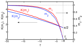
a) b)

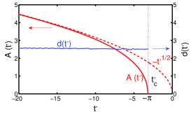
Figure 2: Temperature dependencies of parameters of Eq.(19): (a) elliptic arguments $m_{1}$ and $m_{2}$, elliptic integrals $K_{1}$ and $K_{2}$ , (b) domain amplitude $A$ and domain lattice period $d^{\prime}$. All the variables are dimensionless.

Formula (19) satisfies the boundary conditions

$$P^{\prime}(x^{\prime},z^{\prime})=P^{\prime}(x^{\prime}+2d^{\prime},z^{\prime}),\quad P^{\prime}(x^{\prime},0)=P^{\prime}(x^{\prime},2)=0,$$ (21)

recovers the soft domain structure (18) at $t_{c}^{\prime}$ when $m_{12}(t_{c}^{\prime})=0$, $A(t^{\prime})\sim(t_{c}^{\prime}-t^{\prime})^{1/2}$ and the Kittel-like structure at low $t_{c}^{\prime}$ when $m_{12}(t_{c}^{\prime})\rightarrow 1$, $A(t^{\prime})\simeq(-t^{\prime})^{1/2}$, and gives the domain profile at arbitrary $t^{\prime}$. Parameters $K_{12}(t^{\prime})$ determine the space scale of polarization variation: in dimensional variables the characteristic domain wall thickness is $\xi_{x}(t)=\xi_{0x}/(-t)^{1/2}$ whereas the thickness of the near-surface layer where $P(z)$ restores its equilibrium value is $\sim d/(-t)^{1/2}\cdot(\varkappa_{\parallel}/\epsilon_{\perp})^{1/2}$ (i.e. $\sim d$ at low $t$).

Variation and vanishing of polarization at the sample surface modifies the initial assumption of the Kittel model that polarization is permanent inside domain and resolves the long-standing paradox Landau8 ; StrukovLevanyuk according to which the permanent domain polarization should be reoriented close to sample surface by its own depolarization field that exists in the near-surface layer.

As it follows from our calculations, the nonuniform distribution of polarization pumps the depolarization charge $\rho(r)\sim\text{div}\mathbf{P}$ from the sample surface inside the near-surface layer $\sim d$, reducing the unfavorable depolarization field (justification is given in Appendix) and its energy $\mathcal{E}_{d}\sim{E}^{2}/4\pi\sim 4\pi{P}^{2}$. The price of this - the dumping of the condensation energy $\mathcal{E}_{c}\sim 4\pi{P}^{2}/\epsilon_{\parallel}$ is not so high because $\epsilon_{\parallel}\gg 1$. That’s why we believe that the near-surface polarization vanishing is more effective mechanism to overcome the Kittel paradox in ferroelectrics and reduce the near-surface depolarization energy then the usually assumed Landau8 ; StrukovLevanyuk but rarely observed fractal branching of alternatively oriented permanent-polarization domains near the sample surface.

Polarization decay at the surface is the consequence of the boundary condition $P^{\prime}=0$ of simplified equations (14)-(16). The validity of this effect is illustrated in Fig. 3 where we compare the numerical solution of simplified equations (14)-(16) (Fig. 3b) with that for the complete set of CT equations (Fig. 3a). Clearly the tendency of polarization vanishing is conserved for the case of general solution in Fig. 3a, although the ”real” boundary condition $\partial_{z}P=0$ (8) is satisfied exactly at the surface. Interesting to note that the precursor of the competitive surface domain branching is also seen at Fig. 3ab as ripples at the domain end-points. The corresponding variational solution (19) at Fig. 3c is more smooth, but correctly represents the properties of numerical profile.

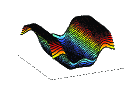
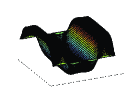
a) b)c)

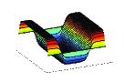
Figure 3: Polarization of Kittel domain. (a) Numerical solution of complete CT equations (6)-(9). (b) Numerical solution of simplified equations (14)-(16). (c) Interpolation formula (19)

We present now several remarkable conclusions about the physical properties of the multi-domain state which can be obtained only from the scaling properties (10), without solution of CT equations (6)-(9).

(i) Any transverse length parameter scales as $\tau^{-1/2}\xi_{0x}$. This, in particular, justifies the Kittel formula (1) for the domain width $d$ even beyond the flat domain approximation. A convincing demonstration of the validity of this scaling law was reported recently for various ferroelectric and ferromagnetic materials 2007Catalan . The temperature dependence $d(t)$ can be incorporated into (1) as dependence $\gamma=\gamma(t)$. Meanwhile, the results shown in Fig. 2b as well as finite-element simulations Guerville indicate that the dependence $d(t)$ is very weak and hence one can extend the parameter $\gamma\simeq 3.53$ from (1) to any temperature.This, in particular, implies the low temperature hysteresis related with motion of DW.

(ii) The temperature $t$ scales as $\tau$. Thus, to compare the domain-provided physical properties of different plates or films (even constructed from different materials) it should be instructive to trace their temperature dependencies using the re-scaled coordinate $t/\tau$.

(iii) All the domain-related properties and, in particular, the transition temperature $t_{c}$ (17) and the soft-to-hard domain crossover temperature $t^{\ast}\sim 10t_{c}$ scale as $1/2a_{f}$ with plate (film) width, as illustrated in Fig. 1c. The temperature interval for the existence of soft-domains $\Delta t=t_{c}-t^{\ast}$ growth dramatically with decreasing film thickness and one can expect that for thin films with $2a_{f}<100nm$ only soft domains with a gradual polarization distribution are possible.

Summarizing we conclude that domains in any ferroelectric sample and at any temperature can be easily obtained from interpolation formulas (19,20) applying the scaling relations (10). This can be especially helpful to treat the experimental data, involving the local field distribution of polarization inside domains like ESR or Raman spectroscopy, TEM domain imagery etc.

We demonstrated that depending on the temperature and sample width domains can have soft (gradual) or hard (Kittel) profile. In any case polarization has the tendency to vanish at sample surface.

Basing on universal scaling relations (10) we have demonstrated how the physical properties of the different multi-domain films can be compared and mapped onto each other. We hope that such method will give the power tool for analysis and systematization of numerous experimental data for thin ferroelectric films.

This work was supported by the Region of Picardy, France, by STREP ”Multiceral”(NMP3-CT-2006-032616) and by FP7 IRSES program ”Robocon”. We thank to Prof. M. G. Karkut for the useful discussions.

APPENDIX (EPAPS document)

We present here the technical derivation of (i) simplified equations and corresponding boundary conditions from the generating Euler-Lagrange functional (ii) interpolation formula for domain polarization (iii) justification of simplification of generating functional.

We use the defined in the article dimensionless variables, omitting the prime index.

(i) Derivation of simplified equations and boundary conditions from the Euler-Lagrange functional

Euler-Lagrange variation of the simplified dimensionless functional(12) that describes ferroelectric phase in a infinite thin plate (film) located at $0<z<2$: over polarization $P$ and potential of electric field $\varphi$ gives:

$$\delta F=\int\left[\begin{array}[]{c}4\pi\left(tP\delta P+P^{3}\delta P+\left(\partial_{x}P\right)(\partial_{x}\delta P\right)\\ -\frac{1}{4\pi}(\partial_{x}\varphi)(\partial_{x}\delta\varphi)+\delta P\partial_{z}+\delta P\partial_{z}\varphi+P\partial_{z}\delta\varphi\end{array}\right]dxdz$$

$$=\begin{array}[]{c}4\pi\int\delta P\left(tP+P^{3}-\partial_{x}^{2}P+\frac{1}{4\pi}\partial_{z}\varphi\right)dxdz\\ -\int\delta\varphi\left(\frac{1}{4\pi}\partial_{x}^{2}\varphi-\partial_{z}P\right)dxdz+\left[\int P\delta\varphi dx\right]_{z=0}^{z=2}\end{array}=0$$

Two first (volume) terms provide the corresponding dimensionless equations (14)-(15) whereas the third (surface) term gives the boundary condition (16)that should be completed by condition of continuity of potential at $z=0$ and at $z=2$.

(ii) Derivation of interpolation formula for domain polarization

Although the nonlinear equations (14)-(16) can not be solved exactly we shall look for their $x$-periodic domain solution in the variational form

$$P = f(z)\,\mathrm{sn}\left[\frac{4K(m_{1})}{2d}\,x,\,m_{1}\right],$$ (22)

$$\qquad f(0) = f(2)=0,\text{ \ }P(x,z)=P(x+d,z)$$

considering $m_{1}$, $d$ and the function $f(z)$ as variational parameters that minimize (12)

Substitution of (22) back into (12) and integration over domain period gives:

$$\int[-\frac{1}{8\pi}(\partial_{x}\varphi)^{2}+P\partial_{z}\varphi]dxdz$$ (23)

$$\overset{(\ref{ne2})}{=}\int[-\frac{1}{8\pi}(\partial_{x}\varphi)^{2}-\frac{1}{4\pi}\varphi\partial_{x}^{2}\varphi]dxdz$$

$$\overset{(\ref{ne2})}{=}2\pi\int\left(\partial_{z}f\right)^{2}\,(2d)^{2}\,\delta(m_{1})dz$$

and

$$\int 4\pi\left(\frac{1}{2}tP^{2}+\frac{1}{4}P^{4}+\frac{1}{2}\left(\partial_{x}P\right)^{2}\right)dxdz$$

$$= 4\pi\int\left(\begin{array}[]{c}\frac{1}{2}tf(z)^{2}\,\alpha(m_{1})+\frac{1}{4}f(z)^{4}\,\eta(m_{1})\\ +\frac{1}{2}f(z)^{2}\,\frac{4K(m_{1})}{\left(2d\right)^{2}}\beta(m_{1})\end{array}\right)dz$$

Now the functional depends only on variable $z$:

$$F=4\pi\int\left[\begin{array}[]{c}\frac{1}{2}\,\left(\alpha(m_{1})t+\,\frac{4K(m_{1})}{\left(2d\right)^{2}}\beta(m_{1})\right)f(z)^{2}\\ +\frac{1}{4}\,\eta(m_{1})f(z)^{4}+\frac{1}{2}\delta(m_{1})\,(2d)^{2}\left(\partial_{z}f\right)^{2}\end{array}\right]dz$$ (25)

where the coefficients are expressed via complete elliptic integrals of the first and second kind $K(m)$, $E(m)$ as:

$$\alpha(m) = <\mathrm{sn}^{2}(x,m)>$$

$$= \frac{1}{m}\left[1-\frac{E(m)}{K(m)}\right]$$

$$\eta(m) = <\mathrm{sn}^{4}(x,m)>$$

$$= \frac{1}{3m}\left[2\left(1+m\right)\alpha(m)-1\right]$$

$$\delta(m) = \frac{\left\langle\mathrm{S}^{2}\left(x,m\right)\right\rangle}{\left[4K(m)\right]^{2}}$$

$$= \frac{8}{m\left[4K(m)\right]^{2}}\sum_{l=1,3,5}^{\infty}\left[\frac{1}{l}\frac{q^{l/2}(m)}{1-q^{l}(m)}\right]^{2}$$

$$\beta(m) = 4K(m)\left\langle\left(\mathrm{sn}^{\prime}u\right)^{2}\right\rangle$$

$$= 4K(m)\frac{1}{3}\left[2-\left(1+m\right)\alpha(m)\right]$$

Here $q(m)=e^{-\frac{K(1-m)}{K(m)}\pi}$, $\mathrm{S}\left(x,m\right)=\int^{x}\mathrm{sn}\left(u,m\right)du$ and $\left\langle\ldots\right\rangle$ is the average over the period.

Dependencies $\alpha(m)$, $\beta(m)$, $\eta(m)$ and $\delta(m)$ are presented in Fig 4.

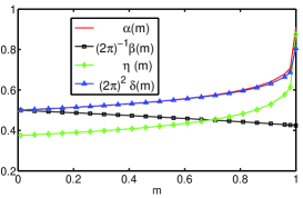
Figure 4: Coefficients $\alpha(m)$, $\beta(m)$, $\gamma(m)$ and $\delta(m)$ that enter into the variational functional (25)

The variational Euler-Lagrange minimum of (25) is given by the function:

$$f(z)=A(t,m_{1},m_{2})\,\mathrm{sn}\left[K(m_{2})\,z,m_{2}\right]$$ (30)

with

$$A(t,m_{1},m_{2})=2d\left(t,m_{1},m_{2}\right)K(m_{2})\,\sqrt{2\frac{\delta(m_{1})}{\eta(m_{1})}m_{2}}$$ (31)

that matches the boundary conditions $f(0)=f(2)=0$ providing that the dependence $d(t,m_{1},m_{2})$ is fixed by biquadratic equation:

$$\begin{array}[]{c}(2d)^{4}\delta(m_{1})(1+m_{2})K^{2}(m_{2})+(2d)^{2}\alpha(m_{1})t\\ +4K(m_{1})\beta(m_{1})\end{array}=0$$ (32)

Substitution of (30) back into (25) gives:

$$F(m_{1},m_{2}) = -4\pi\frac{1}{4}\eta(m_{1})\int f^{4}(z)\,dz$$

$$= -\frac{1}{2}\pi\eta(m_{1})A^{4}(t,m_{1},m_{2})\eta(m_{2})$$

Collecting all the results, we present the final variational solution (19).

(iii) Justification of simplification of generating functional

The simplified functional (12) was obtained by neglecting the terms (13).

Using profile $P(x,z)$ from (19) we can now justify that contribution of these terms is indeed small by noting that their action is concentrated in the near-surface layer of thickness $\xi_{r}\sim 1/K_{2}(t)\sim|t|^{-1/2}$. We will consider only the Kittel regime far from $t_{c}=-\pi$. The soft regime close to $t_{c}$ was already considered in Stephano .

The relative contribution of the first term to $F$ is estimated as

$$\int\widehat{A}_{1}dxdz/F\sim(\frac{\varepsilon_{\perp}}{\varkappa_{\parallel}})^{1/2}\frac{\xi_{0z}}{a_{f}}\xi_{r}\sim(\frac{d}{a_{f}})^{2}|t|^{-1/2}\ll 1$$ (34)

that is small for the Kittel domains with $d\ll a_{f}$. Note, however, that this criteria is not satisfied for monodomain polarization profile that formally is achieved when $d\rightarrow\infty$. This means that dimensionless equations (14,15) can not be applied for monodomain x-independent solution, that however is unstable towards domain formation anyway.

Another term $\widehat{A}_{2}$ is related with the energy of the depolarizing electric field $E_{z}$. According to (15), this field can be calculated from the polarization profile (19) as:

$$E_{z}(x,z)=-\partial_{z}\varphi=-4\pi\partial_{z}^{2}\int\int^{xx_{1}}P(x_{2},z)dx_{2}dx_{1}.$$ (35)

It follows that the depolarization field $E_{z}$ periodically alternates in $x-$direction in anti-phase with $P$ and is located in the near-surface layer of thickness $\xi_{r}$. It vanishes at the surface and in the bulk. Estimating the maximal value of $E_{z}$ at $x\sim\xi_{r}/2$ as $E_{z\max}\sim A$ we have:

$$\int\widehat{A}_{2}dxdz/F\sim\frac{\varepsilon_{i\parallel}}{\varkappa_{\parallel}}(\frac{\varkappa_{\parallel}}{\varepsilon_{\perp}})^{1/2}\frac{\xi_{0x}}{a_{f}}\xi_{r}\sim\frac{\varepsilon_{i\parallel}}{\varkappa_{\parallel}}(\frac{d}{a_{f}})^{2}|t|^{-1/2}\ll 1.$$ (36)

The physical meaning of this estimation is discussed in the main text of the article.

References

(1) M. Dawber, K. M. Rabe and J. F. Scott, Rev. Mod.
Phys., 77, 1083 (2005)
(2) L. Landau and E. Lifshitz, Phys. Z. Sowjet. 8, 153 (1935)
(3) L. D. Landau and E. M. Lifshitz, Electrodynamics
of Continuous Media (Elsevier, New York,1985)
(4) C. Kittel, Phys. Rev. 70, 965 (1946)
(5) A. M. Bratkovsky and A. P. Levanyuk, Phys. Rev.
Lett. 84, 3177 (2000)
(6) F. De Guerville, I. Lukyanchuk, L. Lahoche, and M. El
Marssi, Mat. Sci. and Eng., B120, 16 (2005)
(7) G. Catalan, J. F. Scott, A. Schilling and J. M. Gregg,
J. Phys: Cond. Matter 19 022201 (2007)
(9) E. V. Chensky and V. V. Tarasenko, Sov. Phys. JETP
56, 618 (1982)[Zh. Eksp. Teor. Fiz. 83, 1089 (1982)]
(10) V. A. Stephanovich, I. A. Luk’yanchuk and M. G.
Karkut, Phys. Rev. Lett., 94, 047601 (2005)
(11) Bo-Kuai Lai, I. Ponomareva, I. I. Naumov et al. Phys.
Rev. Lett. 96, 137602 (2006)
(12) D. G. Sannikov, ”Phenomenological Theory of the
Incommensurate-Commensurate Phase Transition” p. 43 in Incommensurete
Phases in Dielectrics I. Fundamentals, ed. by R. Blinc and A. P. Levanyuk,
Elsevier. Sci. Publ., Amsterdam, 1986
(13) Abramowitz M., Stegun I.A. (eds.) Handbook of
mathematical functions (10ed., NBS, 1972)
(14) B. A. Strukov and A. P. Levanyuk, Ferroelectric Phenomena in Crystals (Springer, Berlin,1998)
(15) Frequently used more general boundary condition is obtained when polarization is constrained by
additional surface contribution to free
energy (3). We neglect this term here.
(16) V. A. Stephanovich et al., Phys. Rev. Lett., 94,
047601 (2005)
b)
b)
.
. b)
b)
b)
b) c)
c)