Hidden Symmetries of M-Theory and Its Dynamical Realization

Hidden Symmetries of M-Theory
and Its Dynamical Realization

Alexei J. NURMAGAMBETOV A.J. Nurmagambetov

A.I. Akhiezer Institute for Theoretical Physics, NSC “Kharkov Institute of Physics
and Technology”, 1 Akademicheskaya Str., 61108 Kharkiv, Ukraine

ajn@kipt.kharkov.ua

Received October 31, 2007, in final form February 06, 2008; Published online February 19, 2008

We discuss hidden symmetries of M-theory, its feedback on the construction of the M-theory effective action, and a response of the effective action when locality is preserved. In particular, the locality of special symmetries of the duality-symmetric linearized gravity constraints the index structure of the dual to graviton field in the same manner as it is required to separate the levels 0 and 1 generators subalgebra from the infinite-dimensional hidden symmetry algebra of gravitational theory. This conclusion fails once matter fields are taken into account and we give arguments for that. We end up outlining current problems and development perspectives.

duality; gravity; supergravity

83E15; 83E50; 53Z05

1 Introduction

The hidden symmetry structure of M-theory is a subject of considerable interest during the last decade. It is caused by lacking the complete dynamics of M-theory with non-perturbative degrees of freedom, and by our believe that any progress in understanding the symmetry basis of M-theory is helpful in searching for the underlying dynamical principle.

Substantial progress in this direction was recently achieved within the conjectured, at early stages of the development, algebraic structure of M-theory. This structure is realized as the very-extension of the hidden symmetry algebra of dimensionally reduced ${\rm D}=11$ supergravity [2]. Though many arguments in favor of the conjecture were subsequently found, this subject is currently under debates. Nevertheless, seminal ideas of [2] stimulated the development of a new special type of infinite-dimensional algebras, the so-called very-extended algebras [3], that was resulted in recognizing the special rôle of Kac–Moody-type algebras in M-theory setting [4].

Another important consequence arising from the results of [2, 5] was the duality-symmetric structure those of M-theory bosonic tensor fields which cast the bosonic subsector of ${\rm D}=11$ supergravity. Inclusion of their dual fields is strongly expected once we take non-perturbative degrees of freedom into account. Their realizations may be different, a M5-brane [6, 7] is one of them. Getting of M5-branes requires a sufficient modification of ${\rm D}=11$ supergravity action [8], which becomes duality-symmetric with respect to the third and sixth rank tensor fields. The corresponding generators can be found on the hidden symmetry algebra side [2].

With account of the above-mentioned points, the duality-symmetric ${\rm D}=11$ supergravity action [8] can be considered as a good staring point in searching for the least action principle of hidden constituents of M-theory which are encoded in the symmetry algebra. However, the construction of [8] has to be sufficiently extended with new fields. They would correspond to infinitely many generators of the conjectured very-extended symmetry algebra. Steps on this way are discussed in what follows in more detail.

At the same time we have to point out that the manifestly covariant Lagrangian approach to duality-symmetric theories [9], which is in the focus of the paper, is not the only way to construct the least action principle of M-theory. Other ways (see e.g. [10, 11]), which also exploit the infinite-dimensional structure of the M-theory hidden symmetry algebra, are subjects of recent reviews [4, 12]. The alternative least action principle mentioned there is based on a sigma-model (propagating in one time-like direction, so a particle-type) action invariant under an infinite-dimensional algebra transformations. Realization of this program is very attractive (see [13]), however, some conceptual points should be recovered on the way. For instance, it is a questionable point on the consistent coupling of a dynamical M5-brane and other brane sources to such a sigma-model-type action with retaining the (special) symmetries of branes. Other points of further development are the extension of the ‘dictionary’ between sigma-model variables and space-time fields beyond low-levels (see [10, 12] for details) and the generalization of the approach to the completely supersymmetric case. Nonetheless, one may notice an apparent advantage of the approach: the sigma-model-type action is based on the non-linear realization of the hidden symmetry algebra, hence the feedback of the algebra structure on the sigma-model dynamics is manifest on this way.

The extension of the duality-symmetric ${\rm D}=11$ supergravity action [8], in its bosonic subsector, with the graviton dual field was proposed in [19]. Such an extension required introducing non-locality. The non-locality of the proposed action, the symmetry structure and dynamics were subjects of intensive discussion in our previous paper [20].

In this paper we extend the analysis of the duality-symmetric linearized gravity, made in [20], and establish the restriction on the index structure of the graviton (or vielbein in the first order approach) dual field

$$A_{[a,b_{1}\dots b_{D-3}]}=0,$$

which ensures the locality of the special symmetries (see [9]). Remarkably, the similar constraint, but on the hidden symmetry algebra side, was found in [2, 5]. This constraint separates the subalgebra of generators corresponding to the graviton and to the graviton dual field from the rest of the infinite-dimensional algebra, which is the hidden symmetry algebra of gravitational theory. On our side this constraint is required for retaining the locality of the model, and since the vielbein and its dual partner are related to each other via the duality relation, the constraint on the dual field removes the antisymmetric part of the originally unconstrained vielbein. Put it differently, the locality of the linearized duality-symmetric gravity results in the constraint on the vielbein which leads to the Fierz–Pauli-type linearized spin-2 theory.

We should warn the reader that the obtained result takes place for the pure duality-symmetric linearized gravity. Once matter fields are included, the action of the model becomes non-local and the off-shell locality cannot be kept anymore.

The organization of the paper is as follows. To fix ideas and to make the paper self-contained we briefly review dualities of String Theory and their connection to the hidden symmetries of M-theory (Section 2). Next, we discuss the algebraic structure of M-theory based on [2] (Section 3), and its restriction to the gravity case (Section 4). In Section 5 we discuss the realization of the duality-symmetric gravity [19] within the approach of [9], Section 6 contains extended, in comparison to [20], analysis of the linearized theory. To make a contact to M-theory we consider the duality-symmetric linearized gravity in presence of matter fields (Section 7). We give arguments on the off-shell non-locality in the case, which is general and do not depend on the nature of matter fields. Summing up of the results is made in Conclusions. The notation of the paper can be found in Appendix.

2 String Theory dualities and hidden symmetries

Dualities and hidden symmetries of String Theory are closely related to each other. To realize this relation we begin with the following cartoon of String Theory (Fig. 1).

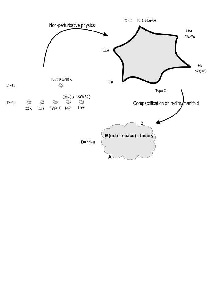
Figure 1: The map of String Theory.

The left part of Fig. 1 is a cartoon of String Theory within the perturbative framework, with six disjoint points of five different superstring theories in ${\rm D}=10$ space-time dimensions and ${\rm D}=11$ $N=1$ supergravity. When non-perturbative degrees of freedom are taken into account it results in M-theory description of String Theory with the same six points, but jointing together. In the bottom of Fig. 1 one finds an effective low-dimensional theory which follows from M-theory after compactifying additional coordinates. Properties of the effective theory are essentially depended on the geometry of internal manifold.

Compactifying M-theory, one arrives at M(oduli space)-theory, which depends on moduli, i.e. some parameters of an effective theory arising upon the compactification. The moduli, but rather transformations of the moduli under (hidden) symmetry groups, form the moduli space, different points of which (points A and B on Fig. 1) correspond to different effective coupling regimes. The effective coupling, say in the A-point, may become weak, so one can study the effective theory perturbatively there. But A and B points of the Moduli space are related to each other via Duality, and it makes possible to predict the behavior of theory in the strong coupling point B by studying the theory in the weak coupling point A.

There are three types of Dualities which connect points in the Moduli space. Annotating on them we will tightly follow [21]. We get started with S-duality, the duality between strong and weak coupling regimes of the same or different type theories. It widely applies for analysis of non-perturbative effects due to Dp-branes, properties of which are collected in Fig. 2.

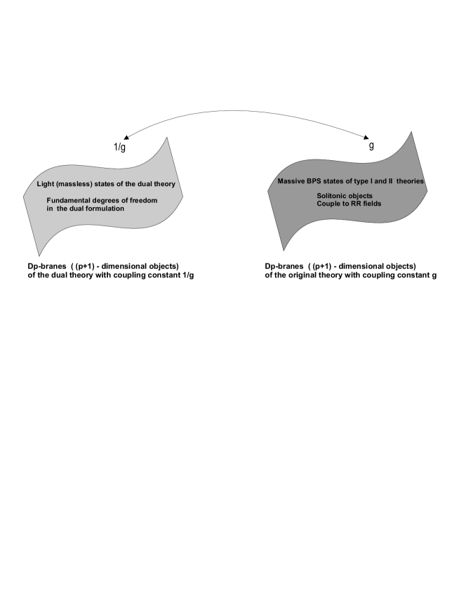
Figure 2: Properties of Dp-branes.

In what follows we will focus on maximally supersymmetric, i.e. type IIA/IIB String Theories. Type IIB superstring theory is invariant under S-duality that, together with the invariance under constant shifts of Ramond–Ramond (RR) fields, results in $SL(2,R)$ symmetry of the theory (which becomes $SL(2,Z)$ after the quantization). On the type IIA side S-duality has a different realization. A stack of $n$ D0-branes with masses $M\sim n/g$ gets transformed into a smooth spectrum of massless particles in the strong coupling constant limit $g\rightarrow\infty$. Such a process may be interpreted as a decompactification of type IIA ${\rm D}=10$ string theory into a ${\rm D}=11$ theory (see Fig. 3).

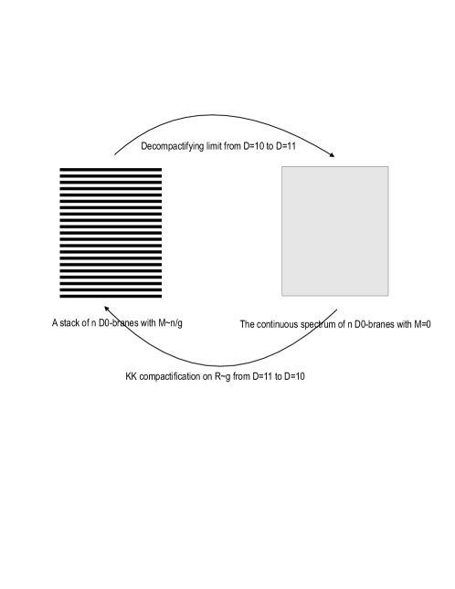
Figure 3: S-duality of type IIA String Theory and M-theory.

Once the latter point is accepted, the spectrum of type IIA $n$ D0-branes naturally arises upon the compactification of ${\rm D}=11$ theory on the circle of radius $R\sim g$. Hence, the strong coupling limit of type IIA theory is indeed a theory in ${\rm D}=11$, referred to as M-theory, and type IIA String Theory is S-dual to M-theory.

Another type of duality, Target-space duality (or T-duality), arises when a string is embedded into a target space of the following configuration ${\cal M}_{D}={\cal M}_{D-n}\times T^{n}$, where $T^{n}$ is a $n$-dimensional internal torus under which a string is wrapped $m$ times (see Fig. 4).

Figure 4: Wrapping of a string on an internal torus.

We are interested in the structure of T-duality group, which can be established as follows. The metric tensor on a $n$-dimensional torus has the same number of degrees of freedom as that of the following coset space

$$\frac{SL(n)}{SO(n)}\times R^{+}.$$

Here $R^{+}$ is the torus volume parameter. Since we are dealing with String Theory, there is also a two-form gauge field $B_{2}$, whose contribution into degrees of freedom on the torus is $\Lambda^{2}R^{n}=n(n-1)/2$. The total contribution of the metric and of the two-form gauge field is matched with the number of degrees of freedom carried by the following coset space

$$\frac{O(n,n)}{O(n)\times O(n)}.$$

The latter is the T-duality group.

What is worth mentioning here is the enhancement of the gravity internal degrees of freedom global symmetry group, from $SL(n)$ to $O(n,n)$, due to the contribution of String Theory gauge field $B_{2}$. We will see in what follows that this statement is general.

We end up with U-duality, which unites the dualities mentioned in the above. To establish the U-duality group, one should study both type IIA/IIB theories in different coupling regimes and in ${\cal M}_{D}={\cal M}_{D-n}\times T^{n}$ space-times. In type IIA picture we have $SL(n)$ to $O(n,n)$ enhancement due to T-duality, and $SL(n)$ to $SL(n+1)$ enlargement through the M-theory interpretation (S-duality). These symmetries jointly generate the larger U-duality group. A convenient way to establish the U-duality group comes as follows [21, 22].

$SL(n)$ algebra corresponds to $A_{n-1}$ Dynkin diagram with $n-1$ nodes (see Fig. 5).

Figure 5: $A_{n-1}$ Dynkin diagram.

The enlargement to $O(n,n)$ corresponds to $D_{n}$ Dynkin diagram with $n$ nodes (Fig. 6), while the enlargement to $SL(n+1)$ algebra gets $A_{n}$ diagram (with $n$ nodes, Fig. 7).

Figure 6: $D_{n}$ Dynkin diagram.

Figure 7: $A_{n}$ Dynkin diagram.

An entanglement of two diagrams, Fig. 6 and Fig. 7, is realized in $E_{n+1}$ diagram, Fig. 8 (with $n+1$ nodes).

Figure 8: $E_{n+1}$ Dynkin diagram.

The latter group is the hidden symmetry global group of String Theory in ${\cal M}_{D}={\cal M}_{D-n}\times T^{n}$ target-space.

A symmetry group of String Theory should also incorporate the symmetry groups of the low-energy effective actions, viz. supergravities. Since ${\cal M}_{D}={\cal M}_{D-n}\times T^{n}$ target space configuration can be interpreted as the toroidal reduction, (a subgroup of) $E_{n+1}$ should appear in the toroidally reduced maximal supergravities. Normally the structure of $E_{n+1}$ is hidden and is recovered after making additional steps like, for example, dualisation of fields.

An interpretation of $E_{n}$ for $n<3$ is subtle (as well as for high $n$, since $E_{8}$ is the end of $E_{n}$ sequence of classical algebras), rather it is a unifying notation for global symmetry groups of the moduli space in the reduced theories. Taking into account the relation of ${\rm D}=11$ $N=1$ supergravity to type IIA supergravity via the reduction on a one-torus, the $E_{n}$ sequence of hidden symmetries can be assigned to the toroidally reduced ${\rm D}=11$ supergravity, and should be incorporated into M-theory. The moduli space of the reduced M-theory in the low-energy approximation is as in Fig. 9.

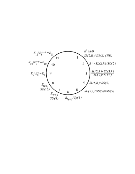
Figure 9: M(oduli)-theory clock.

An amazing fact one can read off Fig. 9 is that when the reduction goes over three-dimensional space-time down to dimensions two, one and zero, the $E_{n}$ sequence of global symmetry algebras still continues. When $n>8$, the global symmetry algebras become Kac–Moody-type infinite-dimensional algebras. It is absolutely unclear why “conspiracy” arises, unless it has presented in the unreduced theory. Following this way, we arrive at the West’s conjecture on $E_{11}$ as a hidden symmetry algebra of M-theory [2].

3 The algebraic structure of $\boldsymbol{E_{11}}$

The conjecture by West [2] is very attractive since we have nothing hidden to search anymore. In its turn, it has several non-trivial corollaries. We have noticed that upon the reduction the symmetry groups get extended from finite-dimensional groups and algebras to infinite-dimensional Kac–Moody-type algebras. Hence M-theory constructed this way contains infinitely many massless fields. Some of them may be auxiliary fields, which do not carry dynamical degrees of freedom. So we have to find the relation between fields corresponding to generators of the Kac–Moody-type algebra and those of perturbative string spectrum.

To make this matching one should know the generators of $E_{11}$. Some of them are easily determined from the $E_{11}$ Dynkin diagram [2, 5].

Deleting the node $11$ results in $A_{10}\sim SL(11)$ algebra. It corresponds to the gravity sector of ${\rm D}=11$ supergravity (the so-called gravity line) [5, 23]. In such a decomposition the simple roots of $E_{11}$ are those of $A_{10}$ and $\alpha_{11}=x-\lambda_{3}$. Here $x$ is orthogonal to the simple roots of $A_{10}$, and $\lambda_{3}$ is one of the fundamental weights of $A_{10}$.

Any root of $E_{11}$ can be written as a combination of simple roots $\alpha=\sum\limits_{i=1}^{10}n_{i}\alpha_{i}+l\alpha_{11}$. The integer $l$ is called the level; it defines the number of times the simple root $\alpha_{11}$ appears in the root decomposition. Our choice of the finite-dimensional subalgebra corresponds to considering the adjoint reps. of $E_{11}$ in terms of the reps. of $A_{10}$.

The following basic facts (see e.g. [25]) are helpful to define the reps. of $E_{11}$ at first three levels: $A^{-1}_{ij}=\lambda_{i}\lambda_{j}$, $i,j=1,\dots,10$ (for simply-laced algebras);

$$A^{-1}_{jk}=\frac{j(11-k)}{11},\quad j\geq k;\qquad A^{-1}_{jk}=A^{-1}_{kj},\quad k\geq j;$$

$\alpha^{2}=2,0,-2,-4,\dots$ (for a Kac–Moody algebra with the symmetric Cartan matrix $A_{ij}$). Summing up the above we get the following generators at levels $0$, $1$, $2$ and $3$ [5]

$$l=0,~{}{K^{a}}_{b}\quad{\mathrm{of}}\quad A_{10};\qquad l=1,~{}R^{[abc]};$$

$$l=2,~{}R^{[abcdef]};\qquad l=3,~{}R^{[abcdefgh],i}.$$

They correspond to graviton, a 3rd rank tensor field of ${\rm D}=11$ SUGRA, its 6th rank dual partner, and the dual to graviton field. There also is another level 3 generator $R^{[abcdefghi]}$, which does not occur in $E_{11}$ since the dimension of a linear space corresponding to this generator (the so-called multiplicity) is equal to zero.

The obtained generators form the following, non-closed, subalgebra [2] which is a part of $E_{11}$

$$[{K^{a}}_{b},{K^{c}}_{d}]=\delta^{c}_{b}{K^{a}}_{d}-\delta^{a}_{d}{K^{c}}_{b},\qquad[{K^{a}}_{b},R^{cde}]=\delta_{b}^{c}R^{ade}+\delta_{b}^{d}R^{aec}+\delta_{b}^{e}R^{acd}\equiv 3\delta_{b}^{[c}R^{|a|de]},$$

$$[R^{abc},R^{def}]=2R^{abcdef},\qquad[R^{abcdef},R^{ghi}]=R^{abcdefgh,i}+R^{abcdefig,h}+R^{abcdefhi,g},$$ (3.1)

$$[{K^{a}}_{b},R^{c_{1}\dots c_{6}}]=6\delta_{b}^{[c_{1}}R^{|a|c_{2}\dots c_{6}]},\quad[{K^{a}}_{b},R^{c_{1}\dots c_{8},d}]=8\delta_{b}^{[c_{1}}R^{|a|c_{2}\dots c_{8}],d}+\delta_{b}^{d}R^{c_{1}\dots c_{8},a}.$$

One can continue constructing the generators (we recall that there are infinitely many generators of $E_{11}$), but they will not be in such a transparent correspondence with fields anymore [27]. Nevertheless, we have got enough information to make an intermediate conclusion: The standard fields of ${\rm D}=11$ SUGRA (the graviton, the 3rd rank tensor field) have to be included together with their duals. Hence, at low-energies, we deal with a duality-symmetric formulation of M-theory.

This point is important in context of the effective dynamical description of M-theory. It is a well-known fact that the construction of ${\rm D}=11$ supergravity action with a 6th rank tensor field instead of the standard antisymmetric tensor gauge field runs into trouble [28, 29]. On the other hand, the 6th rank tensor field is needed for coupling of the dynamical M5-brane [6, 7] to ${\rm D}=11$ supergravity. The problem is only overcome within the duality-symmetric formulation of ${\rm D}=11$ supergravity with 3rd and 6th rank tensor fields [8]. Therefore, the part of the algebra (3.1) corresponding to tensor gauge fields fits very well the dynamics of M-theory with “electric” M2 and “magnetic” M5 branes.

But we still have a question on introducing the gravity into the game. Though the action of [8] has included the Einstein-Hilbert action, it is the incomplete action from the point of view of $E_{11}$. It has to be completed with the graviton dual field.

Another reason to include the graviton dual field into M-theory effective action was noticed in [19]. There we pointed out that the direct way of getting the maximally duality-symmetric type IIA supergravity action (see [14]) through the reduction of the duality-symmetric ${\rm D}=11$ supergravity action requires another starting point than the construction of [8]. Such a ${\rm D}=11$ supergravity formulation should be completely duality-symmetric in the bosonic fields that requires the dualisation of gravity too.

Before doing anything on this way, let us make a comment on (3.1). One may notice that the generator of (3.1), corresponding to the dual to graviton field, appears as an interplay between two generators which correspond to M2 and M5 branes of M-theory. The way of $R^{[abcdefgh],i}$ coming seems to be special, so it is natural to pose the following question: Does including the graviton dual field an artifact of M-theory, or it does appear even in pure gravitational theory?

4 The hidden symmetry algebra of gravitational theory

Long ago it was realized that ${\rm D}=4$ gravity reduced to lower (${\rm D}=3$, ${\rm D}=2$) dimensions possesses unexpected symmetries (the $SL(2,R)$s by Ehlers [30] and by Matzner–Misner [31]). Their interplay leads to an infinite-dimensional group (the Geroch group [32]) which acts on the solutions to the Einstein equation in the background with two commuting Killing vectors [33]. The structure of the Geroch group was established in [34], where it was shown that the infinitesimal form of the Geroch group corresponds to the affine Kac–Moody algebra $SL(2,R)^{+}$.

The Ehlers $SL(2,R)$ is established after dualisation of the Kaluza–Klein vector to a scalar field upon the reduction from ${\rm D}=4$ to ${\rm D}=3$. This scalar (the axion) together with $g_{33}$ component of the metric tensor (the dilaton) form $SL(2,R)/SO(2)$ coset space. The Matzner–Misner $SL(2,R)$ arises upon the direct reduction from ${\rm D}=4$ to ${\rm D}=2$ and corresponds to the global symmetry group of the internal two-torus (the moduli space group).

On account of the discussed $SL(2,R)^{+}$ Geroch algebra of the reduced to ${\rm D}=2$ four-dimensional gravity and its subsequent extension to $SL(2,R)^{++}$ upon the reduction to ${\rm D}=1$ [35], one may expect the very-extended Kac–Moody-type algebra $SL(2,R)^{+++}$ in the end. Following the West’s proposal, this algebra should be the true symmetry algebra of ${\rm D}=4$ gravity. For ${\rm D}$-dimensional gravity this algebra becomes $SL(D-2,R)^{+++}$. Since $SL(2,R)^{+++}\sim A_{1}^{+++}$, the hidden symmetry algebra (for ${\rm D}>3$) is $A_{D-3}^{+++}$.

As for $E_{11}$ one may figure out the generators of $A_{D-3}^{+++}$ classifying them w.r.t. reps. of the gravity line. It corresponds to $A_{D-1}\sim SL(D)$ in the case (see the following Dynkin diagram of $A_{D-3}^{+++}$).

Clearly, we have $A_{D-1}$ generators at level 0 (they are the generators of $SL(D)$), and the generators $R^{[a_{1}\dots a_{D-3}],b}$, $R^{[a_{1}\dots a_{D-3}b]}$ at $l=1$. It is easy to recognize the generator corresponding to the dual to graviton field, $R^{[a_{1}\dots a_{D-3}],b}$, while the last generator does not enter the algebra having the multiplicity zero.

From now on it becomes clear that the presence of the graviton dual field is not an artifact of the $E_{11}$ construction. The corresponding generator enters the symmetry algebra of any theory which contains gravity. For instance, the following subalgebra of ${\rm D}=11$ pure gravity is included in (3.1)

$$[{K^{a}}_{b},{K^{c}}_{d}]=\delta^{c}_{b}{K^{a}}_{d}-\delta^{a}_{d}{K^{c}}_{b},\qquad[{K^{a}}_{b},R^{c_{1}\dots c_{8},d}]=8\delta_{b}^{[c_{1}}R^{|a|c_{2}\dots c_{8}],d}+\delta_{b}^{d}R^{c_{1}\dots c_{8},a},$$ (4.1)

and this non-closed subalgebra is a part of the infinite-dimensional algebra $A_{8}^{+++}$. It is also clear that as soon as the way of constructing the duality-symmetric gravity will be outlined the generalization to the completely duality-symmetric ${\rm D}=11$ supergravity will be almost straightforward.

Before proceeding further, let us make a remark on the index structure of generators of (4.1). The symmetry properties of the gravity line generators ${K^{a}}_{b}$ are not restricted, neither to be completely symmetric nor to be completely antisymmetric. The graviton dual field generators $R^{a_{1}\dots a_{D-3},b}$ are completely antisymmetric over the first $D-3$ indices. However, if we impose the following additional restriction on the index structure

$$R^{[a_{1}\dots a_{D-3},b]}=0,$$ (4.2)

the subalgebra (4.1) splits off the rest of $A_{8}^{+++}$ and forms its closed part. Equation (4.2) is also required to close the algebra (3.1).

5 Duality-symmetric formulation of gravity

We are turning now to the dynamical realization of the duality-symmetric M-theory at low-levels of $E_{11}$. It should include the graviton and its dual field, so we focus first on the construction of the duality-symmetric gravitational theory action.

The following line of reasoning may be helpful in such a quest. The standard gravity action

$$S=\int d^{D}x\,\sqrt{|g|}R$$

depends on the dynamical metric tensor field $g_{mn}=g_{nm}$. To include its dual field, we have to add a new term to the action, which in general depends on the metric tensor, on the graviton dual field $\mathcal{G}$ and its ‘field strength’ ${\mathcal{R}}=\partial\mathcal{G}+\cdots$, and possibly on some auxiliary fields $\xi_{i}$, which are required for different reasons. It could be, for instance, the covariantization of the problem.

The duality-symmetric action becomes

$$S=\int d^{D}x\,\sqrt{|g|}R+\mathcal{L}_{\rm add.}(g,\mathcal{G},\mathcal{R},\xi_{i}),$$ (5.1)

and its variation over the variables leads to the following set of equations of motion

$$R_{mn}-\tfrac{1}{2}g_{mn}R+\frac{\delta\mathcal{L}_{\rm add.}}{\delta g^{mn}}=0,\qquad\frac{\delta\mathcal{L}_{\rm add.}}{\delta\mathcal{G}}=0,\qquad\frac{\delta\mathcal{L}_{\rm add.}}{\delta\xi_{i}}=0.$$ (5.2)

At first glance, equations (5.2) describe the extended, with respect to the original degrees of freedom, dynamical system. However, we require a special form of the new term in (5.1) which, on the one hand, does not spoil the original dynamics (the set of equations (5.2) is reduced to the Einstein equation in the end), and on the other hand, it should contain some specific relations, the duality relations between dual fields, on account of which it could be possible to recover the original dynamics in terms of the dual field.

Another remark concerns the convenient choice of variables to simplify matching with generators of (4.1). We have noted that the generators ${K^{a}}_{b}$ entering (4.1) have the unrestricted index structure. Therefore, they do not correspond to the symmetric metric tensor. But they are well fitted to vielbeins $e^{a}_{m}$, whose index structure is also unrestricted. Moreover, if we treat the upper index of the vielbein as that of an internal symmetry type, and dualize the vielbein over the lower index, similar to a vector field, we precisely recover the dual field, ${A^{a}}_{[m_{1}\dots m_{D-3}]}$, corresponding to the generator $R^{[a_{1}\dots a_{D-3}],b}$. Hence, it is convenient for our purposes to consider gravity in the first order formulation.

Let us make the setting more precise considering the following set of equations

$$\Sigma_{abc}\cdot R^{bc}+\frac{\delta}{\delta e^{a}}\left(v\cdot\mathcal{F}^{a[D-2]}\cdot i_{v}\mathcal{F}^{b[2]}\eta_{ab}\right)=0,$$ (5.3)

$$d(v\cdot i_{v}\mathcal{F}^{a[2]})=0,$$ (5.4)

$$i_{v}\mathcal{F}^{a[D-2]}\cdot d(v\cdot i_{v}\mathcal{F}_{a}^{[2]})+i_{v}\mathcal{F}^{a[2]}\cdot d(v\cdot\mathcal{F}_{a}^{[D-2]})=0.$$ (5.5)

Written in the differential forms notation (see Appendix), equations (5.3)–(5.5) are in exact correspondence to equations (5.2). Equation (5.3) corresponds to the Einstein equation extended with contribution of new additional term, $\mathcal{L}_{\rm add.}$. This term depends on the vielbein $e^{a}$ as well as on the vielbein dual field $A^{a[D-3]}$ through the following generalized field strengths

$$\mathcal{F}^{a[2]}=de^{a}-\ast(dA^{a[D-3]}+\ast\tilde{G}^{a[2]}),$$ (5.6)

$$\mathcal{F}^{a[D-2]}=-\ast\mathcal{F}^{a[2]}.$$ (5.7)

The exact definition of $\ast\tilde{G}^{a[2]}$ is not important for the present discussion, so we skip it for a while. The rest is a one-form [9]

$$v=\frac{da(x)}{{\sqrt{-\partial_{m}a~{}g^{mn}~{}\partial_{n}a}}},$$

constructed out the auxiliary scalar field $a(x)$. $\eta_{ab}$ is apparently reserved for the tangent space Minkowski metric tensor.

One may notice that at least one particular solution to equations (5.3)–(5.5), $\mathcal{F}^{a[2]}=0$, reduces this system to the single Einstein equation. Moreover, this particular solution corresponds to one of the first-order in derivatives duality relations between fields which effectively contain the second order dynamical equations. Taking the external derivative of $\mathcal{F}^{a[2]}=0$ we obtain the dynamics of gravity in terms of the dual field

$$d(\ast dA^{a[D-3]})+\dots=0,$$ (5.8)

while applying the derivative to the second duality relation, $\mathcal{F}^{a[D-2]}=0$, results in the following form of the Einstein equation

$$R_{mn}-\tfrac{1}{2}g_{mn}R\equiv d(\ast de_{a})-{\ast}{\tilde{J}}^{[1]}_{a}=0.$$ (5.9)

The exact expression of the “current” ${\tilde{J}}^{[1]}_{a}$ has the following, convenient for further references, form

$${\tilde{J}}^{[1]}_{a}=(-)^{\frac{D(D-5)}{2}}{J}^{[1]}_{a}+{\ast}d{S}^{[D-2]}_{a},$$ (5.10)

with

$${J}^{[1]}_{a}={\ast}\big{[}{\omega}^{bc}({e})\cdot d{\Sigma}_{{a}{b}{c}}+(-)^{D-3}~{}{{\omega}}^{b}_{~{}{d}}({e})\cdot{\omega}^{{d}{c}}({e})\cdot{\Sigma}_{{a}{b}{c}}\big{]},$$ (5.11)

and

$${S}^{[D-2]}_{a}={\ast}({e}^{b}\cdot{e}_{a}){e}^{m}_{c}{e}^{n}_{b}\partial_{[{m}}{e}^{c}_{{n}]}.$$

Note that (5.11) involves the resolved connection

$${\omega}^{{a}{b}}({e})=\tfrac{1}{2}{e}^{c}\big{[}{e}^{m}_{c}{e}^{{n}{a}}\partial_{[{m}}{e}_{{n}]}^{b}-{e}^{m}_{c}{e}^{{n}{b}}\partial_{[{m}}{e}_{{n}]}^{a}-{e}^{{n}{a}}{e}^{{s}{b}}\partial_{[{n}}{e}_{{s}]{c}}\big{]},$$ (5.12)

which follows from the torsion free constraint

$$T^{a}\equiv de^{a}-{\omega^{a}}_{b}\cdot e^{b}=0,$$ (5.13)

as in the so-called “one and half” formalism (see [36]).

Equations (5.3)–(5.5) together with equation (5.13) can be derived from the first order action [19, 20] (see Appendix for the notation)

$$S=\int_{{\mathcal{M}}^{D}}\,R^{ab}\cdot\Sigma_{ab}+\tfrac{1}{2}v\cdot\mathcal{F}^{a[D-2]}\cdot i_{v}\mathcal{F}^{b[2]}\eta_{ab}.$$ (5.14)

The first term of (5.14) is the standard Einstein–Hilbert–Palatini action and the second one is a slightly generalized PST term [9]. The special structure of the latter is important to prove that the duality relation $\mathcal{F}^{a[2]}=0$ is the general solution to equation (5.4) (see [20] in the case), and that the scalar field $a(x)$ is the auxiliary field. Indeed, on the mass-shell $\mathcal{F}^{a[2]}=0$, the equation of motion of $a(x)$, equation (5.5), is identically satisfied, and does not carry any additional dynamical information.

Finally, $\tilde{G}^{a[2]}$ entering (5.6) is defined by $d\ast\tilde{G}^{a[2]}=\ast\tilde{J}^{a[1]}$. The presence of $\tilde{G}^{a[2]}$ sacrifices the locality of the action, and of the generalized field strengths (5.6), (5.7). However, the dual field equation of motion (5.8) can be rewritten in the local form after the dual field redefinition [20].

6 Duality-symmetric gravity in the linearized approximation

There are numerous indications that the linearized gravity admits dualisation in the local form (see e.g. [37, 38, 39, 40, 41, 42, 43, 44, 45, 46]), and solely in terms of the dual field. However, the generalization of the construction to the non-linear case should be resulted in a duality-symmetric theory. The reasons for that are as follows.

As for bosonic fields, the field dual to graviton has to be described by a second order, in space-time derivatives, equation of motion. Its structure in a curved background is

$$\Box({\mathrm{dual~{}f\/ield}})+\dots=0,$$

where $\dots$ corresponds to possible self-interactions and interactions with the background gravity field. The box $\Box$ is the d’Alembertian operator, and this operator is constructed out the space-time derivatives and the background metric. The dual field dynamics within the full non-linear self-consistent theory (which takes into account the backreaction of the graviton dynamics) will contain the d’Alembertian with the dynamical (non-background) metric. Therefore, the resulted theory will be a duality-symmetric theory which manages the dynamics of both fields, the graviton and its dual partner.

Our previous consideration [20] of the duality-symmetric gravity linearization has indicated that on-shell we encounter the local formulation. Here we would like to extend the analysis to check the locality of the linearized duality-symmetric gravity off-shell.

Let us make a quick recap of the on-shell linearized formulation. We expand the vielbein near the flat space

$${e}^{a}(x)=dX^{m}u^{a}_{m}+{\mathcal{E}}^{a}(x),$$ (6.1)

with a constant matrix $u^{a}_{m}$. The spin connection (5.12) linear in $\mathcal{E}^{a}(x)$ then becomes

$${\omega}^{{a}{b}}({e})\cong\tfrac{1}{2}dX^{k}u^{c}_{k}\big{[}u^{m}_{c}u^{{n}{a}}\partial_{[{m}}{\mathcal{E}}^{b}_{{n}]}-u^{m}_{c}u^{{n}{b}}\partial_{[{m}}{\mathcal{E}}^{a}_{{n}]}-u^{{n}{a}}u^{{s}{b}}\partial_{[{n}}{\mathcal{E}}_{{s}]{c}}\big{]}+\mathcal{O}({\mathcal{E}}^{2}),$$ (6.2)

that means

$${J}^{[1]}_{a}\cong\mathcal{O}({\mathcal{E}}^{2}).$$ (6.3)

Hence the latter expression does not enter the linearized equation of motion. Furthermore,

$${S}^{[D-2]}_{a}={\ast}\left(dX^{k}u^{b}_{k}\cdot dX^{l}u_{{l}{a}}\right)u^{m}_{c}u^{n}_{b}\partial_{[{m}}{\mathcal{E}}^{c}_{{n}]}+\mathcal{O}({\mathcal{E}}^{2})\equiv{\mathbb{S}}^{[D-2]}_{a}+\mathcal{O}({\mathcal{E}}^{2}).$$

In effect, equation of motion (5.9) becomes

$$d({\ast}d{\mathcal{E}}_{a}-{\mathbb{S}}^{[D-2]}_{a})=0,$$ (6.4)

and it has the structure of the Bianchi identity $d(\cdots)=0$ of the dual field strength. This expression is apparently local, so the non-locality corresponding to a self-interacting part of the non-linear action disappears in the linearized limit.

So far we discussed the linearized limit on-shell. Having the on-shell locality does not guarantee the locality off-shell. Let us check the locality of the linearized action and the action symmetries.

The covariant action for the duality-symmetric gravity in the linearized limit is

$$S=\int_{{\mathcal{M}}^{D}}\left([R^{ab}\cdot\Sigma_{ab}]_{\tt{lin.}}+\tfrac{1}{2}v\cdot\mathcal{F}^{m[D-2]}\cdot i_{v}\mathcal{F}^{n[2]}\eta_{mn}\right).$$ (6.5)

The first term of (6.5) is the linearized Einstein–Hilbert–Palatini action and the second term is the linearized version of the PST term of (5.14).

The generalized field strengths which enter (6.5) are defined by

$$\mathcal{F}_{m}^{[D-2]}\equiv\mathcal{F}_{a}^{[D-2]}u_{m}^{a}=\left(dA_{a}^{[D-3]}-(\ast d\mathcal{E}_{a}-{\mathbb{S}}_{a}^{[D-2]})\right)u^{a}_{m},\qquad\mathcal{F}_{m}^{[2]}=-\ast\mathcal{F}_{m}^{[D-2]},$$ (6.6)

and there is no difference between flat and curved indices in the limit. Clearly, the linearized action (6.5) does not contain non-local constituents, hence we encounter the locality at the level of action. But what about the action symmetries?

The covariance of the model is guaranteed by the PST-like construction of the action, and the local Lorentz transformations, which act on the tangent flat space indices, also become truly local (see [20] for details). The remainder is the special symmetries of the approach, the so-called PST symmetries [9], to the analysis of which we are turning now.

Varying the action results in

$$\delta S=\int_{{\mathcal{M}}^{D}}\left(\delta A^{{m}[D-3]}+\frac{\delta a}{{\sqrt{-(\partial a)^{2}}}}i_{v}{\mathcal{F}}^{{m}[D-2]}\right)\eta_{{m}{n}}\cdot d({v}\cdot i_{v}{\mathcal{F}}^{{n}[2]})$$

$$\phantom{\delta S=}{}+\int_{{\mathcal{M}}^{D}}\left(\delta\mathcal{E}^{m}+\frac{\delta a}{{\sqrt{-(\partial a)^{2}}}}i_{v}{\mathcal{F}}^{{m}[2]}\right)\eta_{{m}{n}}\cdot d({v}\cdot i_{v}{\mathcal{F}}^{{n}[D-2]})$$

$$\phantom{\delta S=}{}-\int_{{\mathcal{M}}^{D}}\delta{\mathbb{S}}^{{m}[D-2]}\eta_{{m}{n}}\cdot{v}\cdot i_{v}{\mathcal{F}}^{{n}[2]}.$$ (6.7)

The first two terms of (6.7) vanish under the following transformations of fields

$$\delta a({x})=0,\qquad\delta\mathcal{E}^{m}=da\cdot{\varphi}^{{m}[0]},\qquad\delta A^{{m}[D-3]}=da\cdot{\varphi}^{{m}[D-4]},$$ (6.8)

$$\delta a({x})=\Phi({x}),\qquad\!\delta\mathcal{E}^{m}=-\frac{\Phi}{{\sqrt{-(\partial a)^{2}}}}i_{v}{\mathcal{F}}^{{m}[2]},\qquad\!\delta A^{{m}[D-3]}=-\frac{\Phi}{{\sqrt{-(\partial a)^{2}}}}i_{v}{\mathcal{F}}^{{m}[D-2]}\!\!\!\!\!$$ (6.9)

with local gauge parameters $\varphi^{m[0]}$, $\varphi^{m[D-4]}$, $\Phi$. However, the third term of (6.7) does not generally vanish under (6.8), (6.9).

Indeed, the variation of this term under (6.8) results in

$$\delta{\mathbb{S}}^{{m}[D-2]}\eta_{{m}{n}}\cdot{v}\cdot i_{v}{\mathcal{F}}^{{n}[2]}\sim v_{s}\partial_{k}\varphi^{s[0]}(v^{m}{\mathcal{F}_{m}}^{kl}v_{l}-v^{k}{\mathcal{F}_{m}}^{ml}v_{l})-\partial_{s}\varphi^{s[0]}{\mathcal{F}_{m}}^{ml}v_{l}.$$

One may notice that this variation is equal to zero once

$$u^{a}_{m}\mathcal{F}_{a,[np]}=u^{a}_{m}\mathcal{F}_{[a,np]}.$$

In its turn, (6.6) requires

$$u^{a}_{m}\mathcal{F}_{a,[n_{1}\dots n_{D-2}]}=u^{a}_{m}\mathcal{F}_{[a,n_{1}\dots n_{D-2}]},$$

that leads to

$$u^{a}_{m}A_{[a,n_{1}\dots n_{D-3}]}=0.$$ (6.10)

The invariance of the action under the second special symmetry (6.9) also imposes the constraint (6.10). Once this constraint is relaxed, the PST transformations of the dual field $A^{m[D-3]}$ receive non-local corrections.

The encountered constraint on the dual field index structure corresponds, on the hidden symmetry algebra side, to equation (4.2). Recall, the latter is required to close the subalgebra (4.1).

7 Linearized gravity with matter fields and its dualisation

Having discussed the locality of the duality-symmetric linearized gravity action based on the algebra (4.1), let us take a further step towards the dynamical realization of the M-theory algebra (3.1).

To make a contact to M-theory we have to extend the action (6.5) at least with a three-form field kinetic term. Once this gauge field is taken into account, the expansion of the vielbein (cf. (6.1)) gets modified to the following form

$$e^{a}(x)=\tilde{e}^{a}(x)+\mathcal{E}^{a}(x),$$ (7.1)

where $\tilde{e}^{a}(x)$ is the solution to the linearized Einstein equation with the 3-form field energy-momentum tensor. Putting it differently, we have to expand over the curve background in the case rather than over the flat space-time as it has been done before.

The difference between a curve space and the Minkowski flat space becomes clear once we present (5.12) as

$$\omega^{ab}(e)=\tfrac{1}{2}e^{c}{\Omega_{c}}^{ab}(e,\partial e),$$

so expanding the vielbein as in (7.1) we schematically get

$$\omega^{ab}(e)\cong\tfrac{1}{2}\tilde{e}^{c}{\Omega_{c}}^{ab}(\tilde{e},\partial\mathcal{E})+\tfrac{1}{2}\mathcal{E}^{c}{\Omega_{c}}^{ab}(\tilde{e},\partial\tilde{e})+\mathcal{O}(\mathcal{E}^{2})+\cdots.$$

Clearly, the latter expansion contains the part linear in the bare $\mathcal{E}^{a}$ which was absent in the pure gravity case (see (6.2)). As a result, (6.3) gets modified with terms linear in $\mathcal{E}^{a}$, and equation (6.4) becomes (for ${\rm D}=11$)

$$d(\ast d\mathcal{E}_{a}-{S}^{[9]}_{a})=-\ast J_{a}^{[1]}.$$ (7.2)

The r.h.s. of (7.2) cannot be transformed into a local curl. Put it differently, dualisation of the linearized gravity with matter requires introducing non-locality. The “current” form $\ast\tilde{J}_{a}^{[1]}$ of (5.10) is closed but not exact in the case, so its “pre-current” form $\ast\tilde{G}^{[2]}_{a}$ ($d\ast\tilde{G}^{[2]}_{a}=\ast\tilde{J}_{a}^{[1]}$) is a non-local expression. Since the “pre-current” enters the duality relations (cf. (5.6), (5.7)) its non-locality induces the non-locality of the action. Then, symmetries of the action also become non-local, and (6.10) does not save the locality.

To make our consideration less formal let us reformulate things in more familiar fashion. We will do that for ${\rm D}=4$ linearized gravity with matter; the generalization to a higher-dimensional case is straightforward. The pure linearized gravity action is as follows

$$A=\int\,d^{4}x\,\partial_{a}h_{bc}\mathcal{M}^{abcijk}\partial_{i}h_{jk}.$$ (7.3)

Here $h_{ab}=h_{ba}$ is the linearized graviton field and

$$\mathcal{M}^{abcijk}=(\eta^{ai}\eta^{bc}\eta^{jk}-\eta^{ai}\eta^{bj}\eta^{ci}+2\eta^{ak}\eta^{bj}\eta^{ci}-2\eta^{ak}\eta^{bc}\eta^{ij})_{\rm symm.}.$$ (7.4)

We use the notation of [47]; the symmetry properties of (7.4) is apparent from (7.3).

Equation of motion which follows from (7.3) can be written in the following form

$$\tilde{\mathcal{M}}^{abcijk}\partial_{a}\partial_{i}h_{jk}=0,$$ (7.5)

with $\tilde{\mathcal{M}}^{abcijk}=\eta^{ai}\eta^{bc}\eta^{jk}-\eta^{ai}\eta^{bj}\eta^{ci}+\eta^{ak}\eta^{bj}\eta^{ci}-\eta^{ak}\eta^{bc}\eta^{ij}-\eta^{ic}\eta^{jk}\eta^{ab}+\eta^{ak}\eta^{cj}\eta^{bi}$. Equation (7.5) is the Bianchi identity of the dual to graviton field, ${U_{rs}}^{|bc}$, which is defined by

$$\epsilon^{aprs}\partial_{p}{U_{rs}}^{|bc}=\tilde{\mathcal{M}}^{abcijk}\partial_{i}h_{jk}.$$ (7.6)

So, the dualisation is straightforward and does not violate the locality.

When the matter source is taken into account, equation (7.5) gets transformed into

$$\tilde{\mathcal{M}}^{abcijk}\partial_{a}\partial_{i}h_{jk}=T^{bc}.$$ (7.7)

Here $T^{bc}$ is the energy-momentum tensor of matter fields. Its structure (see, e.g., [47, 48] for details) is as follows

$$T^{bc}\equiv\left[\partial^{c}\phi_{A}\left(\frac{\partial L}{\partial(\partial_{b}\phi_{A})}\right)-\eta^{bc}L\right]+\partial_{a}\psi^{abc},$$

where $\psi^{abc}=-\psi^{bac}$ is an arbitrary third rank tensor. Then, equation (7.7) becomes

$$\partial_{a}\left(\tilde{\mathcal{M}}^{abcijk}\partial_{i}h_{jk}-\psi^{abc}\right)=\left[\partial^{c}\phi_{A}\left(\frac{\partial L}{\partial(\partial_{b}\phi_{A})}\right)-\eta^{bc}L\right],$$ (7.8)

which is nothing but equation (7.2) written in terms of other variables. For a general Lagrangian $L(\phi_{A},\partial_{a}\phi_{A})$ it is quite unexpectable that the r.h.s. of (7.8) can be presented as a local curl.

Moreover, it cannot be done anyway. If it were done it would be possible, due to a 3rd rank tensor $\psi^{abc}$, to ‘neutralize’ the contribution of matter fields to the energy-momentum tensor. Thus, the energy-momentum tensor could always be set to zero, and the dynamics of gravity with matter fields would be the same as the dynamics of pure gravitational field. Presumably, the latter is wrong that completes our arguments.

Therefore, the dualisation of the linearized gravity with matter fields cannot be generally done in the local form. It does not depend on the nature of matter fields $\phi_{A}$ which would be scalar, spinor, vector, tensor or spin-tensor fields.

8 Conclusions

We conclude with the following points. Dualities and hidden symmetries of String Theory are closely related to each other. It has been shown that Dualities of String Theory require the modification of String Theory to M-theory. The algebraic structure of M-theory is encoded in hidden symmetries of the String Theory low-energy effective actions. Such an algebraic structure may be realized dynamically in different ways. Here we have followed [9, 8, 19, 20].

An essential feature of [19, 20] is non-locality of the non-linear action and of the symmetries of the approach. Here we have focused on the locality of the linearized duality-symmetric gravity action. We have observed that the requirement of locality of the linearized duality-symmetric gravity leads to the constraint on the index structure of the dual field (see (6.10)). The corresponding constraint was previously found on the hidden symmetry of M-theory [2, 5] side. Note that this constraint has nothing to do with the action of the model (6.5) which is local, as well as with the equations of motion which follow from the local action. We have observed that this constraint ensures the locality of the special gauge transformations, equations (6.8), (6.9), of the linearized duality-symmetric gravity action. It points at an interesting and quite unexpected relation between the dynamical local symmetries of the action and properties of the hidden symmetry algebra. Furthermore, since the vielbein and the dual field are related to each other through the duality relations (6.6), the constraint (6.10) eliminates the antisymmetric component of the vielbein ${\mathcal{E}_{[m}}^{n]}$, hence leading to the Fierz–Pauli-type description of the spin-2 duality-symmetric linearized theory.

The encountered constraint, on the hidden symmetry algebra side, is responsible for closing the subalgebra of the graviton and of the dual field generators. It leaves no room for other fields corresponding to the Kac–Moody-type algebra, inclusion of which would be helpful, for instance, in quantum description of the model. Recall that the amplitude of the spin-2 single-particle exchange violates the Froissart bound, breaking Unitarity at high energies. Unitarity can be restored but within the Regge poles theory, where the single-particle exchange is replaced with the Reggeon exchange, with a bunch of infinitely many particles belonging to the Regge trajectory. It is natural to query whether the fields of the Kac–Moody algebra has a similar correspondence to the spin-2 field as in the Regge theory, but an answer is unclear for a while.

On the other hand, when the constraint is imposed, we have just a well-defined, from the point of view of the locality, duality-symmetric theory, symmetries of which are the standard for the approach and are well-defined too. If one would try to make the embedding of the symmetries into an extended symmetry structure, one should introduce compensator fields, which would ‘un-Higgs’ the system, thus restoring the large symmetry. Following this way, we could notice that indeed some of the compensators would be the true Higgs fields responsible for the generation of masses of other compensators.

Progress in these directions could be achieved on the way of establishing the correspondence between string theory higher spin modes and those of the appropriate Kac–Moody algebra. An interesting problem solution to which may help on this way is to relax the constraint on the dual to the vielbein field, and to include other fields of the Kac–Moody hidden symmetry algebra into the construction of the duality-symmetric action.

Finally, let us make a short remark on the sigma-model approach of [10, 11, 12, 13]. This approach is based on the conjecture which claims that the full geometrical data of M-theory (and ${\rm D}=11$ supergravity as its low-energy limit as well) can be mapped onto a geodesic motion in the $E_{10}/K(E_{10})$ coset space. The established there ‘dictionary’ between parameters of the coset space and M-theory fields works good up to the third level of $E_{10}$ decomposition with respect to $SL(10)$ finite subalgebra. At the third level, where the dual to graviton field appears, there is a mismatch between the dynamics of the coset space parameters and that of ${\rm D}=11$ supergravity bosonic fields. Such a discrepancy may be resolved with taking into account higher levels of $E_{10}$ on both sides of the correspondence or with taking into account a ‘gradient’ conjecture of [10]. The latter is equivalent to introducing the (spatial) non-locality into the theory. We have encountered the non-locality in the duality-symmetric theory of gravity with matter fields, so the question is how to realize the ‘gradient’ conjecture on our side.

Appendix A Notation and conventions

Our choice of the signature is the mostly minus. Letters from the middle of the Latin alphabet are reserved for the curved indices, letters from the beginning are used for the indices in tangent space. The Levi-Civita tensor $\epsilon^{a_{1}\cdots a_{D}}$ is defined by

$$\epsilon^{01\dots(D-1)}=1,\qquad\epsilon_{01\dots(D-1)}=(-)^{D-1},$$

that implies

$$\epsilon^{a_{1}\dots a_{D}}\epsilon_{a_{1}\dots a_{D}}=(-)^{D-1}D!.$$

An $n$-form has the following coordinate representation

$$\omega^{[n]}=\frac{1}{n!}dx^{m_{n}}\cdots dx^{m_{1}}\omega^{[n]}_{m_{1}\dots m_{n}},$$

and the exterior derivative acts from the right.

The Hodge star is defined by

$$\ast\big{(}dx^{k_{n}}\cdots dx^{k_{1}}\big{)}=\frac{1}{(D-n)!}\frac{\alpha_{n}}{\sqrt{|g|}}\,dx^{m_{D-n}}\cdots dx^{m_{1}}{\epsilon_{m_{1}\dots m_{D-n}}}^{k_{1}\dots k_{D-n}},$$

with coefficients $\alpha_{n}$ fixed to provide the universal identity $\ast^{2}=1$.

The curvature of $SO(1,D-1)$ connection $\omega^{ab}$ is $R^{ab}=d\omega^{ab}-{\omega^{a}}_{c}\cdot\omega^{cb}$,

$$\Sigma_{a_{1}\dots a_{n}}=\frac{1}{(D-n)!}\epsilon_{a_{1}\dots a_{D}}e^{a_{n+1}}\cdot\dots\cdot e^{a_{D}}$$

is a $(D-n)$-form constructed out of vielbeins $e^{a}$. The wedge product between forms is supposed.

Acknowledgements

Discussions with Igor Bandos, Martin Cederwall, Vladimir Lyakhovsky, Dmitri Sorokin, Kellog Stelle, Mikhail Vasiliev, Dmitri Vassilevich, Yuri Zinoviev are kindly acknowledged. Work supported in part by the INTAS grant #05-1000008-7928.

References

- [1]
- [2] West P.C., and M-theory, Classical Quantum Gravity 18 (2001), 4443–4460, hep-th/0104081.
- [3] Gaberdiel M.R., Olive D.I., West P.C., A class of Lorentzian Kac–Moody algebras, Nuclear Phys. B 645 (2002), 403–437, hep-th/0205068.
- [4] Buyl S., Kac–Moody algebras in M-theory, hep-th/0608161 (and references therein).
- [5] West P.C., Very extended and at low levels, gravity and supergravity, Classical Quantum Gravity 20 (2002), 2393–2406, hep-th/0212291.
- [6] Bandos I., Lechner K., Nurmagambetov A., Pasti P., Sorokin D., Tonin M., Covariant action for super-five-brane of M theory, Phys. Rev. Lett. 78 (1997), 4332–4335, hep-th/9701149.
- [7] Aganagic M., Park J., Popescu C., Schwarz J.H., World-volume action of the M theory five-brane, Nuclear Phys. B 496 (1997), 191–214, hep-th/9701166.
- [8] Bandos I., Berkovits N., Sorokin D., Duality-symmetric eleven-dimensional supergravity and its coupling to M-branes, Nuclear Phys. B 522 (1998), 214–233, hep-th/9711055.
-
[9]
Pasti P., Sorokin D., Tonin M., Note on manifest Lorentz and general coordinate invariance in duality symmetric models, Phys. Lett. B 352 (1995), 59–63, hep-th/9503182.
Pasti P., Sorokin D., Tonin M., Duality symmetric actions with manifest space-time symmetries, Phys. Rev. D 52 (1995), 4277–4281, hep-th/9506109.
Pasti P., Sorokin D., Tonin M., On Lorentz invariant actions for chiral -forms, Phys. Rev. D 55 (1997), 6292–6298, hep-th/9611100. - [10] Damour T., Henneaux M., Nicolai H., and a “small tension expansion” of M-theory, Phys. Rev. Lett. 89 (2002), 221601, 4 pages, hep-th/0207267.
- [11] Englert F., Houart L., invariant formulation of gravity and M-theories: exact BPS solutions, J. High Energy Phys. 2004 (2004), no. 1, 002, 45 pages; hep-th/0311255.
- [12] Henneaux M., Persson D., Spindel Ph., Spacelike singularities and hidden symmetries of gravity, arXiv:0710.1818.
- [13] Damour T., Nicolai H., Symmetries, singularities and the de-emergence of space, arXiv:0705.2643.
- [14] Bandos I.A., Nurmagambetov A.J., Sorokin D.P., Various faces of type IIA supergravity, Nuclear Phys. B 676 (2004), 189–228, hep-th/0307153.
- [15] Cremmer E., Julia B., Lü H., Pope C.N., Dualisation of dualities II: Twisted self-duality of doubled fields and superdualities, Nuclear Phys. B 535 (1998), 242–292, hep-th/9806106.
- [16] Nurmagambetov A.J., The sigma-model representation for the duality-symmetric supergravity, in Proceedings of Fifth International Conference “Symmetry in Nonlinear Mathematical Physics” (June 23–29, 2003, Kyiv), Editors A.G. Nikitin, V.M. Boyko, R.O. Popovych and I.A. Yehorchenko, Proceedings of Institute of Mathematics, Kyiv 50 (2004), Part 2, 894–901, hep-th/0312157.
- [17] Nurmagambetov A.J., Sigma-model-like action for type IIA supergravity in doubled field approach, in Proceedings of International Workshop SQS’03 (July 24–29, 2003, Dubna), 2003, 84–89.
- [18] Nurmagambetov A.J., On the sigma-model structure of type IIA supergravity action in doubled field approach, JETP Lett. 79 (2004), 191–195, hep-th/0403100.
- [19] Nurmagambetov A.J., Duality-symmetric gravity and supergravity: testing the PST approach, Ukr. J. Phys. 51 (2006), 330–338, hep-th/0407116.
- [20] Nurmagambetov A.J., Duality-symmetric approach to General Relativity and supergravity, SIGMA 2 (2006), 020, 34 pages, hep-th/0602145.
- [21] Morrison D.R., TASI lectures on compactification and duality, hep-th/0411120.
- [22] Nurmagambetov A.J., On E(11) of M-theory: 1. Hidden symmetries of maximal supergravities and LEGO of Dynkin diagrams, in Proceedings of II International Conference on QED and Statistical Physics (September 19–23, Kharkov, Ukraine), Problems of Atomic Science and Technology 3 (2007), 51–55.
- [23] Lambert N.D., West P.C., Coset symmetries in dimensionally reduced bosonic string theory, Nuclear Phys. B 615 (2001), 117–132, hep-th/0107209.
- [24] Nurmagambetov A.J., Diagrammar and metamorphosis of coset symmetries in dimensionally reduced type IIB supergravity, JETP Lett. 79 (2004), 355–359, hep-th/0403101.
- [25] Kac V.G., Infinite dimensional Lie algebras, Birkhäuser, Boston, 1983.
- [26] Bergshoeff E., Nutma T.A., De Baetselier I., and the embedding tensor, arXiv:0705.1304.
- [27] Kleinschmidt A., Schnakenburg I., West P.C., Very-extended Kac–Moody algebras and their interpretation at low levels, Classical Quantum Gravity 21 (2004), 2493–2525, hep-th/0309198.
- [28] Nicolai H., Townsend P.K., Nieuwenhuizen P., Comments on 11-dimensional supergravity, Lett. Nuovo Cimento 30 (1981), 315–320.
- [29] D’Auria R., Fre P., Geometric supergravity in and its hidden supergroup, Nuclear Phys. B 201 (1982), 101–140, Erratum, Nuclear Phys. B 206 (1982), 496.
- [30] Ehlers J., Les théories relativistes de la gravitation, CNRS, Paris, 1959.
- [31] Matzner R., Misner C., Gravitational field equations for sources with axial symmetry and angular momentum, Phys. Rev. 154 (1967), 1229–1232.
- [32] Geroch R., A method for generating solutions of Einstein’s equations, J. Math. Phys. 12 (1971), 918–924.
- [33] Breitenlohner P., Maison D., On the Geroch group, Ann. Inst. H. Poincaré 46 (1987), 215–246.
- [34] Julia B., Kac–Moody symmetry of gravitation and supergravity theories, AMS-SIAM Seminar Proceedings, Chicago, 1982, Preprint LPTENS-82-22, 1982, 25 pages.
- [35] Nicolai H., A hyperbolic Lie algebra from supergravity, Phys. Lett. B 276 (1992), 333–340.
- [36] van Nieuwenhuizen P., Supergravity, Phys. Rep. 68 (1981), 189–398.
- [37] Garcia-Compean H., Obregon O., Plebansky J.F., Ramirez C., Towards a gravitational analogue to S-duality in non-Abelian gauge theories, Phys. Rev. D 57 (1998), 7501–7506, hep-th/9711115.
- [38] Garcia-Compean H., Obregon O., Ramirez C., Gravitational duality in MacDowell–Mansouri gauge theory, Phys. Rev. D 58 (1998), 104012, 3 pages, hep-th/9802063.
- [39] Nieto J.A., S-duality for linearized gravity, Phys. Lett. A 262 (1999), 274–281, hep-th/9910049.
- [40] Hull C.M., Gravitational duality, branes and charges, Nuclear Phys. B 509 (1998), 216–251, hep-th/9705162.
- [41] Hull C.M., Strongly coupled gravity and duality, Nuclear Phys. B 583 (2000), 237–259, hep-th/0004195.
- [42] Hull C.M., Duality in gravity and higher spin gauge fields, J. High Energy Phys. 2001 (2001), no. 9, 027, 25 pages, hep-th/0107149.
- [43] Boulanger N., Cnockaert S., Henneaux M., A note on spin-s duality, J. High Energy Phys. 2003 (2003), no. 6, 060, 18 pages, hep-th/0306023.
- [44] Henneaux M., Teitelboim C., Duality in linearized gravity, Phys. Rev. D 71 (2005), 024018, 8 pages, gr-qc/0408101.
- [45] Julia B., Levie J., Ray S., Gravitational duality near de Sitter space, J. High Energy Phys. 2005 (2005), no. 11, 025, 13 pages, hep-th/0507262.
- [46] Ajith K.M., Harikumar E., Sivakumar M., Dual linearized gravity in arbitrary dimensions, Classical Quantum Gravity 22 (2005), 5385–5396, hep-th/0411202.
- [47] Padmanabhan T., From graviton to gravity: myths and reality, gr-qc/0409089.
- [48] Leclerc M., Canonical and gravitational stress-energy tensors, Internat. J. Modern Phys. D 15 (2006), 959–990, gr-qc/0510044.