KUNS-2126 $D_{4}$ Flavor Symmetry for Neutrino Masses and Mixing

Abstract

We present the $D_{4}\times Z_{2}$ flavor symmetry, which is different from the previous work by Grimus and Lavoura. Our model reduces to the standard model in the low energy and there is no FCNC at the tree level. Putting the experimental data, parameters are fixed, and then the implication of our model is discussed. The condition to realize the tri-bimaximal mixing is presented. The possibility for stringy realization of our model is also discussed.

1 Introduction

It is the important task to find an origin of the observed hierarchies in masses and flavor mixing for quarks and leptons. Neutrino experimental data provide us an important clue for this task. Especially, recent experiments of the neutrino oscillation go into the new phase of precise determination of mixing angles and mass squared differences [1, 2]. Those indicate the tri-bimaximal mixing for three flavors in the lepton sector [3]. Therefore, it is necessary to find a natural model that leads to this mixing pattern with good accuracy.

Flavor symmetries, in particular non-Abelian discrete flavor symmetries, are interesting ideas to realize realistic patterns of mass matrices. Actually, several types of models with non-Abelian discrete flavor symmetries have been proposed [4]. Furthermore, non-Abelian discrete flavor symmetries can be realized in the simple geometrical understanding of superstring theory [5, 6] as well as extra dimensional models. The $D_{4}$ symmetry can appear typically in heterotic string models on factorizable orbifolds including the $Z_{2}$ orbifold. Indeed, several semi-realistic models with $D_{4}$ flavor symmetries have been constructed in Ref. [5, 7] and in those models three families correspond to a singlet and a doublet under the $D_{4}$ flavor symmetry. Therefore, taking $D_{4}$ symmetry as the flavor symmetry of quarks and leptons, these mass spectra and the flavor mixing matrix should be carefully examined to establish the realistic model of quarks and leptons [8, 9].

The $D_{4}$ flavor symmetry was at first proposed for the neutrino mass matrix by Grimus and Lavoura [8]. In this model, the atmospheric neutrino mixing is maximal while the solar neutrino mixing is arbitrary. They introduced three electroweak Higgs doublets together with two neutral singlets in the scalar sector to reproduce the large flavor mixing angles. Then, the tree level flavor changing neutral scalar vertices do not vanish. Moreover, when we consider supersymmetric extension of this $D_{4}$ flavor model, such a supersymmetric model would have three pairs of up and down Higgs fields. That would violate the gauge coupling unification, which is one of important aspects of the minimal supersymmetric standard model, unless one introduces extra colored supermultiplets.

In this paper, we propose alternative $D_{4}$ flavor model with one Higgs doublet, which reduces to the standard model in the low energy. There is no tree level flavor changing neutral current (FCNC) in our model. The higher dimensional operators provide the charged lepton and neutrino masses. Putting the experimental data, our parameters are fixed, and then the implication of our model is discussed.

The paper is organized as follows: we present the framework of the $D_{4}$ model in Sec. 2, and discuss the neutrino masses, flavor mixing angles and Higgs potential in Sec. 3. In Sec. 4, the numerical results are discussed. Section 5 is devoted to the summary and discussion.

2 $D_{4}$ flavor symmetry and Yukawa couplings

We present the framework of our $D_{4}$ flavor model. The $D_{4}$ symmetry has five irreducible representations, that is, a doublet $2$ and four singlets, $1_{++}$, $1_{+-}$, $1_{-+}$ and $1_{--}$, where $1_{++}$ is a trivial singlet and the others are non-trivial singlets. Their products are decomposed as

$$2\times 2=1_{++}+1_{+-}+1_{-+}+1_{--},\qquad 1_{ab}\times 1_{cd}=1_{ef},$$ (1)

where $a,b,c,d=\pm$, $e=ac$ and $f=bd$. Here, the left-handed lepton doublets are denoted as $l_{\alpha}\ (\alpha=e,\mu,\tau)$ and the right-handed charged leptons and right-handed neutrinos are denoted as $e_{R},\mu_{R},\tau_{R}$, $N_{e},N_{\mu},N_{\tau}$, respectively. The first family leptons are assigned to $D_{4}$ trivial singlets, while second and third family ones are to $D_{4}$ doublets. The electroweak Higgs doublet $h$ is a $D_{4}$ trivial singlet. We summarize charges of flavor symmetry in Table 1, where new gauge singlet scalar fields $\chi$, $\chi_{-+}$, $\chi_{1}$, $\chi_{2}$ are introduced and additional $Z_{2}$ charges are assigned for leptons and scalars.

	$l_{e}$	$(l_{\mu},l_{\tau})$	$e_{R}$	$(\mu,\tau)_{R}$	$N_{e}$	$(N_{\mu},N_{\tau})$	$h$	$\chi$	$\chi_{-+}$	$(\chi_{1},\chi_{2})$
$D_{4}$	$1_{++}$	2	$1_{++}$	2	$1_{++}$	2	$1_{++}$	$1_{++}$	$1_{-+}$	2
$Z_{2}$	+	+	$-$	$-$	+	+	+	$-$	$-$	+

Table 1: $D_{4}$ and $Z_{2}$ charges given for leptons and scalars.

2.1 Charged lepton mass matrix

We write down the Yukawa interactions, which are invariant under the gauge group of the standard model and the flavor symmetry $D_{4}\times Z_{2}$, by using the multiplication rule of $D_{4}$ in Eq. (1),

$$-{\cal L}_{l} = y_{e}\bar{e}l_{e}h\chi+y_{\tau}(\bar{\mu}l_{\mu}+\bar{\tau}l_{\tau})h\hat{\chi}+y^{\prime}_{\tau}(-\bar{\mu}l_{\mu}+\bar{\tau}l_{\tau})h\hat{\chi}_{-+}$$ (2)

$$+y_{e\tau}\bar{e}(l_{\mu}\hat{\chi}_{1}+l_{\tau}\hat{\chi}_{2})h\hat{\chi}+y^{\prime}_{e\tau}\bar{e}(l_{\mu}\hat{\chi}_{1}-l_{\tau}\hat{\chi}_{2})h\hat{\chi}_{-+}$$

$$+y_{\tau e}(\bar{\mu}\hat{\chi}_{1}+\bar{\tau}\hat{\chi}_{2})l_{e}h\hat{\chi}+y^{\prime}_{\tau e}(\bar{\mu}\hat{\chi}_{1}+\bar{\tau}\hat{\chi}_{2})l_{e}h\hat{\chi}_{-+}$$

$$+y^{a}_{\mu\tau}(\bar{\mu}\hat{\chi}_{1}+\bar{\tau}\hat{\chi}_{2})(l_{\mu}\hat{\chi}_{1}+l_{\tau}\hat{\chi}_{2})h\hat{\chi}+y^{b}_{\mu\tau}(\bar{\mu}\hat{\chi}_{1}-\bar{\tau}\hat{\chi}_{2})(l_{\mu}\hat{\chi}_{1}-l_{\tau}\hat{\chi}_{2})h\hat{\chi}$$

$$+y^{c}_{\mu\tau}(\bar{\mu}\hat{\chi}_{2}+\bar{\tau}\hat{\chi}_{1})(l_{\mu}\hat{\chi}_{2}+l_{\tau}\hat{\chi}_{1})h\hat{\chi}+y^{d}_{\mu\tau}(\bar{\mu}\hat{\chi}_{2}-\bar{\tau}\hat{\chi}_{1})(l_{\mu}\hat{\chi}_{2}-l_{\tau}\hat{\chi}_{1})h\hat{\chi}$$

$$+y^{\prime}{}^{a}_{\mu\tau}(\bar{\mu}\hat{\chi}_{1}+\bar{\tau}\hat{\chi}_{2})(l_{\mu}\hat{\chi}_{1}-l_{\tau}\hat{\chi}_{2})h\hat{\chi}_{-+}+y^{\prime}{}^{b}_{\mu\tau}(\bar{\mu}\hat{\chi}_{1}-\bar{\tau}\hat{\chi}_{2})(l_{\mu}\hat{\chi}_{1}+l_{\tau}\hat{\chi}_{2})h\hat{\chi}_{-+}$$

$$+y^{\prime}{}^{c}_{\mu\tau}(\bar{\mu}\hat{\chi}_{2}+\bar{\tau}\hat{\chi}_{1})(l_{\mu}\hat{\chi}_{2}-l_{\tau}\hat{\chi}_{1})h\hat{\chi}_{-+}+y^{\prime}{}^{d}_{\mu\tau}(\bar{\mu}\hat{\chi}_{2}-\bar{\tau}\hat{\chi}_{1})(l_{\mu}\hat{\chi}_{2}+l_{\tau}\hat{\chi}_{1})h\hat{\chi}_{-+}$$

$$+\cdots+h.c.,$$

where $\hat{\chi}$ and $\hat{\chi}_{-+}$ denote $\chi/\Lambda$ and $\chi_{-+}/\Lambda$ respectively, and $\Lambda$ is the cutoff scale. The scale $\Lambda$ is taken to be the Planck one in our numerical study. The ellipsis in Eq. (2) denotes higher order contributions but they are negligibly small in our considerations.

We take the vacuum expectation values of scalar fields as follows:

$$\left<h\right>=v,\quad\left<(\chi_{1},\chi_{2})\right>=(V_{1},V_{2}),\quad\left<\chi\right>=V_{a},\quad\left<\chi_{-+}\right>=V_{b}\ ,$$ (3)

where $v=174{\rm GeV}$ and others are taken to be $D_{4}$ symmetry breaking scale. After spontaneous symmetry breaking, the mass matrix of charged lepton becomes

$$M_{l} = v\left[\begin{array}[]{ccc}y_{e}\alpha_{a}&(y_{e\mu}\alpha_{a}-y^{\prime}_{e\mu}\alpha_{b})\alpha&(y_{e\mu}\alpha_{a}+y^{\prime}_{e\mu}\alpha_{b})\alpha\\ (y_{\mu e}\alpha_{a}-y^{\prime}_{\mu e}\alpha_{b})\alpha&y_{\tau}\alpha_{a}-y^{\prime}_{\tau}\alpha_{b}&(y_{\mu\tau}\alpha_{a}+y^{\prime}_{\mu\tau}\alpha_{b})\alpha^{2}\\ (y_{\mu e}\alpha\alpha_{a}+y^{\prime}_{\mu e}\alpha_{b})\alpha&(y_{\mu\tau}\alpha_{a}-y^{\prime}_{\mu\tau}\alpha_{b})\alpha^{2}&y_{\tau}\alpha_{a}+y^{\prime}_{\tau}\alpha_{b}\\ \end{array}\right],$$ (7)

where $\alpha_{a}\equiv V_{a}/\Lambda$ and $\alpha_{b}\equiv V_{b}/\Lambda$ and we assume the vacuum alignment in the $D_{4}$ doublet scalar field, $V_{1}=V_{2}$, so that, $\left<(\chi_{1},\chi_{2})\right>=(V,V)$. The parameter $\alpha$ is defined as $\alpha\equiv V/\Lambda$. This vacuum alignment is important for the masses and mixings in the neutrino sector. Since the value of $\alpha$ is sufficiently small as discussed later, the charged lepton mass matrix can be approximately regarded as diagonal. The masses of charged leptons are given by

$$m_{e}=y_{e}\alpha_{a}v,\quad m_{\mu}=y_{\tau}\alpha_{a}v-y^{\prime}_{\tau}\alpha_{b}v,\quad m_{\tau}=y_{\tau}\alpha_{a}v+y^{\prime}_{\tau}\alpha_{b}v.$$ (8)

We need the fine-tuning to obtain the difference between the masses of the muon and the tau, $m_{\mu}/m_{\tau}\ll 1$, as discussed in Ref. [8].

2.2 Neutrino mass matrix

Let us consider the neutrino sector. We can write down the possible Dirac mass terms up to the dimension five operators by the same prescription as the charged lepton sector,

$$-{\cal L}_{D} = y_{1}\bar{N}_{e}l_{e}\tilde{h}+y_{2}(\bar{N}_{\mu}l_{\mu}+\bar{N}_{\tau}l_{\tau})\tilde{h}$$ (9)

$$+y_{12}\bar{N}_{e}(l_{\mu}\hat{\chi}_{1}+l_{\tau}\hat{\chi}_{2})\tilde{h}+y_{21}(\bar{N}_{\mu}\hat{\chi}_{1}+N_{\tau}\hat{\chi}_{2})l_{e}\tilde{h}$$

$$+y^{a}_{23}(\bar{N}_{\mu}\hat{\chi}_{1}+\bar{N}_{\tau}\hat{\chi}_{2})(l_{\mu}\hat{\chi}_{1}+l_{\tau}\hat{\chi}_{2})\tilde{h}$$

$$+y^{b}_{23}(\bar{N}_{\mu}\hat{\chi}_{1}-\bar{N}_{\tau}\hat{\chi}_{2})(l_{\mu}\hat{\chi}_{1}-l_{\tau}\hat{\chi}_{2})\tilde{h}$$

$$+y^{c}_{23}(\bar{\mu}\hat{\chi}_{2}+\bar{\tau}\hat{\chi}_{1})(l_{\mu}\hat{\chi}_{2}+l_{\tau}\hat{\chi}_{1})\tilde{h}$$

$$+y^{d}_{23}(\bar{\mu}\hat{\chi}_{2}-\bar{\tau}\hat{\chi}_{1})(l_{\mu}\hat{\chi}_{2}-l_{\tau}\hat{\chi}_{1})\tilde{h}$$

$$+\cdots+h.c.\ ,$$

where $\tilde{h}=i\tau_{2}h^{*}$. The Majorana mass terms are given as

$${\cal L}_{R} = M_{1}N_{e}^{T}C^{-1}N_{e}+M_{2}(N_{\mu}^{T}C^{-1}N_{\mu}+N_{\tau}^{T}C^{-1}N_{\tau})$$ (10)

$$+y_{a}N_{e}^{T}C^{-1}(N_{\mu}\chi_{1}+N_{\tau}\chi_{2})$$

$$+y^{a}_{b}(N_{\mu}^{T}\chi_{1}+N_{\tau}^{T}\chi_{2})C^{-1}(N_{\mu}\chi_{1}+N_{\tau}\chi_{2})/\Lambda$$

$$+y^{b}_{b}(N_{\mu}^{T}\chi_{1}-N_{\tau}^{T}\chi_{2})C^{-1}(N_{\mu}\chi_{1}-N_{\tau}\chi_{2})/\Lambda$$

$$+y^{c}_{b}(N_{\mu}^{T}\chi_{2}+N^{T}_{\tau}\chi_{1})C^{-1}(N_{\mu}\chi_{2}+N_{\tau}\chi_{1})/\Lambda$$

$$+y^{d}_{b}(N_{\mu}^{T}\chi_{2}-N_{\tau}^{T}\chi_{1})C^{-1}(N_{\mu}\chi_{2}-N_{\tau}\chi_{1})/\Lambda$$

$$+\cdots+h.c.$$

Then the neutrino mass matrices of Dirac $M_{D}$ and Majorana $M_{R}$ are given by

$$M_{D} = v\left(\begin{array}[]{ccc}y_{1}&y_{12}\alpha&y_{12}\alpha\\ y_{21}\alpha&y_{2}&y_{23}\alpha^{2}\\ y_{21}\alpha&y_{32}\alpha^{2}&y_{2}\\ \end{array}\right),\qquad M_{R}=\left(\begin{array}[]{ccc}M_{1}&y_{a}\Lambda\alpha&y_{a}\Lambda\alpha\\ y_{a}\Lambda\alpha&M_{2}&y_{b}\Lambda\alpha^{2}\\ y_{a}\Lambda\alpha&y_{b}\Lambda\alpha^{2}&M_{2}\\ \end{array}\right).$$ (17)

Similarly to the case of charged leptons, the ellipses in Eqs. (9) and (10) correspond to higher order contributions but they are negligible.

The neutrino mass matrix is given by the see-saw mechanism,

$$M_{\nu}=M_{D}M_{R}^{-1}M_{D}^{T}.$$ (18)

The neutrino mass matrix has the following structure,

$$M_{\nu} \approx v^{2}\left(\begin{array}[]{ccc}A&B&B\\ B&C&D\\ B&D&C\\ \end{array}\right),$$ (22)

where

$$A = \frac{y_{1}^{2}M_{2}^{2}}{M_{1}M_{2}^{2}-2\alpha^{2}\Lambda^{2}M_{2}y_{a}^{2}},\qquad B=-\frac{y_{1}y_{2}y_{a}\alpha\Lambda M_{2}}{M_{1}M_{2}^{2}-2\alpha^{2}y_{a}^{2}\Lambda^{2}M_{2}},$$

$$C = \frac{y_{2}^{2}(M_{1}M_{2}-y_{a}^{2}\alpha^{2}\Lambda^{2})}{M_{1}M_{2}^{2}-2\alpha^{2}y_{a}^{2}\Lambda^{2}M_{2}},\qquad D=\frac{y_{2}^{2}y_{a}^{2}\alpha^{2}\Lambda^{2}}{M_{1}M_{2}^{2}-2\alpha^{2}y_{a}^{2}\Lambda^{2}M_{2}}.$$ (23)

In these expressions, higher order terms are neglected under the assumption of

$$M_{1}M_{2}^{2}\gg\alpha^{4}\Lambda^{3},\quad M_{2}\gg\alpha^{2}M_{1},\quad M_{2}\gg\alpha^{2}\Lambda,\quad\Lambda\gg M_{1}\ .$$ (24)

These assumptions are justified by the numerical analyses as discussed later. The neutrino mass matrix is diagonalized by the following mixing matrix,

$$V=\left(\begin{array}[]{ccc}c&s&0\\ -s/\sqrt{2}&c/\sqrt{2}&1/\sqrt{2}\\ -s/\sqrt{2}&c/\sqrt{2}&-1/\sqrt{2}\\ \end{array}\right),$$ (28)

where $c\equiv\cos\theta_{12}$ and $s\equiv\sin\theta_{12}$ and $\theta_{12}$ corresponds to the solar mixing angle [8]. Then the neutrino mass matrix Eq. (22) is represented by the solar mixing and neutrino mass eigenvalues $m_{i}$ $(i=1\sim 3)$ such as $M_{\nu}=V\mathrm{diag}(m_{1},m_{2},m_{3})V^{T}$, which is

$$\left(\begin{array}[]{ccc}A&B&B\\ B&C&D\\ B&D&C\\ \end{array}\right)v^{2}$$ (32)

$$=\left(\begin{array}[]{ccc}c^{2}m_{1}+s^{2}m_{2}&-cs(m_{1}-m_{2})/\sqrt{2}&-cs(m_{1}-m_{2})/\sqrt{2}\\ -cs(m_{1}-m_{2})/\sqrt{2}&(s^{2}m_{1}+c^{2}m_{2}+m_{3})/2&(s^{2}m_{1}+c^{2}m_{2}-m_{3})/2\\ -cs(m_{1}-m_{2})/\sqrt{2}&(s^{2}m_{1}+c^{2}m_{2}-m_{3})/2&(s^{2}m_{1}+c^{2}m_{2}+m_{3})/2\\ \end{array}\right)\ ,$$ (36)

and we have the relations,

$$Av^{2}=c^{2}m_{1}+s^{2}m_{2},\quad Bv^{2}=-\frac{cs}{\sqrt{2}}(m_{1}-m_{2}),\quad$$

$$Cv^{2}=\frac{1}{2}(s^{2}m_{1}+c^{2}m_{2}+m_{3}),\quad Dv^{2}=\frac{1}{2}(s^{2}m_{1}+c^{2}m_{2}-m_{3}).$$ (38)

For neutrino masses, we find

$$m_{1}+m_{2} = \left(A+C+D\right)v^{2}\ ,$$

$$m_{1}-m_{2} = -\frac{\sqrt{2}}{cs}Bv^{2}\ ,$$

$$m_{3} = Cv^{2}-Dv^{2}\ .$$ (39)

Then, the mass squared differences and the solar mixing angle are expressed by

$$\Delta m_{\mathrm{atm}}^{2} = -\frac{1}{4}\left(A+C+D-\frac{\sqrt{2}}{cs}B\right)^{2}v^{4}+\left(C-D\right)^{2}v^{4},$$

$$\Delta m_{\mathrm{sol}}^{2} = \left(A+C+D\right)\frac{\sqrt{2}}{cs}Bv^{4},$$

$$\cot 2\theta_{12} = \frac{1}{2\sqrt{2}B}\left(C-A+D\right).$$ (40)

2.3 Potential analysis

Here, we analyze the scalar potential and discuss the assumption of vacuum alignment, $V_{1}=V_{2}$. The relevant scalar potential of ($\chi$, $\chi_{-+}$, $\chi_{1}$, $\chi_{2}$) is given by

$$-{\cal L}_{v} = -\mu_{1}^{2}\chi^{2}-\mu_{2}^{2}\chi_{-+}^{2}-\mu_{3}^{2}(\chi_{1}^{2}+\chi_{2}^{2})$$

$$+\lambda_{1}\chi^{4}+\lambda_{2}\chi_{-+}^{4}+\lambda_{3a}(\chi_{1}^{2}+\chi_{2}^{2})^{2}+\lambda_{3b}(\chi_{1}^{2}-\chi_{2}^{2})^{2}+\lambda_{3c}\chi_{1}^{2}\chi_{2}^{2}$$

$$+\lambda_{12}\chi^{2}\chi_{-+}^{2}+\lambda_{13}\chi^{2}(\chi_{1}^{2}+\chi_{2}^{2})+\lambda_{23}\chi_{-+}^{2}(\chi_{1}^{2}+\chi_{2}^{2})+\lambda_{123}\chi\chi_{-+}(\chi_{1}^{2}-\chi_{2}^{2}).$$

The minimum conditions are

$$\frac{\partial{\cal L}_{v}}{\partial\chi} = 2V_{a}\left(-\mu_{1}^{2}+2\lambda_{1}V_{a}^{2}+\lambda_{12}V_{b}^{2}+\lambda_{13}(V_{1}^{2}+V_{2}^{2})+\lambda_{123}\frac{V_{b}}{2V_{a}}(V_{1}^{2}-V_{2}^{2})\right)=0,$$

$$\frac{\partial{\cal L}_{v}}{\partial\chi_{-+}} = 2V_{b}\left(-\mu_{2}^{2}+2\lambda_{2}V_{b}^{2}+\lambda_{12}V_{a}^{2}+\lambda_{23}(V_{1}^{2}+V_{2}^{2})+\lambda_{123}\frac{V_{a}}{2V_{b}}(V_{1}^{2}-V_{2}^{2})\right)=0,$$

$$\frac{\partial{\cal L}_{v}}{\partial\chi_{1}} = 2V_{1}\left(\frac{}{}-\mu_{3}^{2}+2\lambda_{3a}(V_{1}^{2}+V_{2}^{2})+2\lambda_{3b}(V_{1}^{2}-V_{2}^{2})+\lambda_{3c}V_{2}^{2}\right.$$

$$\left.+\lambda_{13}V_{a}^{2}+\lambda_{23}V_{b}^{2}+\lambda_{123}V_{a}V_{b}\frac{}{}\right)=0,$$

$$\frac{\partial{\cal L}_{v}}{\partial\chi_{2}} = 2V_{2}\left(\frac{}{}-\mu_{3}^{2}+2\lambda_{3a}(V_{1}^{2}+V_{2}^{2})-2\lambda_{3b}(V_{1}^{2}-V_{2}^{2})+\lambda_{3c}V_{1}^{2}\right.$$ (42)

$$\left.+\lambda_{13}V_{a}^{2}+\lambda_{23}V_{b}^{2}-\lambda_{123}V_{a}V_{b}\frac{}{}\right)=0.$$

Since there are sixteen parameters ($\mu_{1,2,3}$, $\lambda_{1,2,3a,3b,3c}$, $\lambda_{12,13,23,123}$, $V_{a,b,1,2}$) while there are four equations, these equations can be solved. For this analysis, the following relation is important,

$$(4\lambda_{3b}-\lambda_{3c})(V_{1}^{2}-V_{2}^{2})+2\lambda_{123}V_{a}V_{b}=0,$$ (43)

which is derived from $\partial{\cal L}_{v}/\partial\chi_{1}=0$ and $\partial{\cal L}_{v}/\partial\chi_{2}=0$. To align the vacuum of $V_{1}=V_{2}$, one requires $\lambda_{123}=0$, which is an assumption in our model. We may impose additional symmetry to realize $\lambda_{123}=0$. Inserting $\lambda_{123}=0$, we have

$$V_{a}^{2} = \frac{(2\lambda_{2}\lambda_{3}-2\lambda_{23}^{2})\mu_{1}^{2}+(2\lambda_{13}\lambda_{23}-\lambda_{12}\lambda_{3})\mu_{2}^{2}+(2\lambda_{12}\lambda_{23}-4\lambda_{2}\lambda_{13})\mu_{3}^{2}}{4\lambda_{1}\lambda_{2}\lambda_{3}+4\lambda_{12}\lambda_{13}\lambda_{23}-4\lambda_{1}\lambda_{23}^{2}-4\lambda_{2}\lambda_{13}^{2}-\lambda_{3}\lambda_{12}^{2}},$$

$$V_{b}^{2} = \frac{(2\lambda_{13}\lambda_{23}-\lambda_{12}\lambda_{3})\mu_{1}^{2}+(2\lambda_{1}\lambda_{3}-2\lambda_{13}^{2})\mu_{2}^{2}+(2\lambda_{12}\lambda_{13}-4\lambda_{1}\lambda_{23})\mu_{3}^{2}}{4\lambda_{1}\lambda_{2}\lambda_{3}+4\lambda_{12}\lambda_{13}\lambda_{23}-4\lambda_{1}\lambda_{23}^{2}-4\lambda_{2}\lambda_{13}^{2}-\lambda_{3}\lambda_{12}^{2}},$$

$$V^{2} = \frac{(\lambda_{12}\lambda_{23}-2\lambda_{2}\lambda_{13})\mu_{1}^{2}+(\lambda_{12}\lambda_{13}-2\lambda_{1}\lambda_{23})\mu_{2}^{2}+(4\lambda_{1}\lambda_{2}-\lambda_{12}^{2})\mu_{3}^{2}}{4\lambda_{1}\lambda_{2}\lambda_{3}+4\lambda_{12}\lambda_{13}\lambda_{23}-4\lambda_{1}\lambda_{23}^{2}-4\lambda_{2}\lambda_{13}^{2}-\lambda_{3}\lambda_{12}^{2}},$$ (44)

where $\lambda_{3}\equiv 4\lambda_{3a}+\lambda_{3c}$. It is found that we can take $V_{a}\sim V_{b}$, which is necessary to obtain muon and tau masses by adjusting parameters.

3 Numerical discussion

Let us discuss our numerical results. We define the following two dimensionless parameters, which are the ratios of $M_{2}$ and $\alpha\Lambda$ to $M_{1}$, respectively,

$$r\equiv\frac{M_{2}}{M_{1}}\ ,\quad k\equiv\frac{\alpha\Lambda}{M_{1}}\ .$$ (45)

By using these parameters and Eq. (2.2), the mass squared differences and the solar mixing angle are rewritten as

$$\Delta m_{\mathrm{atm}}^{2} = \frac{-(y_{1}^{2}r^{2}+y_{2}^{2}r+\sqrt{2}y_{1}y_{2}y_{a}kr/cs)^{2}/4+y_{2}^{4}(r-2y_{a}^{2}k^{2})^{2}}{(r^{2}-2y_{a}^{2}k^{2}r)^{2}}\cdot\frac{v^{4}}{M_{1}^{2}}\ ,$$

$$\Delta m_{\mathrm{sol}}^{2} = \frac{-\sqrt{2}y_{1}y_{2}y_{a}kr(y_{1}^{2}r^{2}+y_{2}^{2}r)}{(r^{2}-2y_{a}^{2}k^{2}r)^{2}cs}\cdot\frac{v^{4}}{M_{1}^{2}}\ ,$$

$$\cot 2\theta_{12} = \frac{y_{1}^{2}r-y_{2}^{2}}{2\sqrt{2}y_{1}y_{2}y_{a}k}\ .$$ (46)

The neutrino masses are given as

$$m_{1} = \frac{1}{2}\cdot\frac{y_{a}^{2}r^{2}+y_{2}^{2}r+\sqrt{2}y_{1}y_{2}y_{a}kr/cs}{r^{2}-2y_{a}^{2}k^{2}r}\times\frac{v^{2}}{M_{1}},$$

$$m_{2} = \frac{1}{2}\cdot\frac{y_{a}^{2}r^{2}+y_{2}^{2}r-\sqrt{2}y_{1}y_{2}y_{a}kr/cs}{r^{2}-2y_{a}^{2}k^{2}r}\times\frac{v^{2}}{M_{1}},$$

$$m_{3} = \frac{y_{2}^{2}(r-2y_{a}^{2}k^{2})}{r^{2}-2y_{a}^{2}k^{2}r}\times\frac{v^{2}}{M_{1}}.$$ (47)

When we put the best fit values of mass squared differences and the solar mixing angle as $\Delta m_{\rm atm}^{2}=2.4\times 10^{-3}$eV², $\Delta m_{\rm sol}^{2}=7.6\times 10^{-5}$eV², and $\sin^{2}\theta_{12}=0.32$ [1], we have typical values of parameters in this model,

$$r=0.12,\qquad k=-0.80,\qquad M_{1}=4.9\times 10^{15}{\rm GeV},$$ (48)

where we take all Yukawa couplings as $y_{1}=y_{2}=y_{a}=y_{b}=1$. By taking the cutoff scale $\Lambda$ as the Planck scale $2.43\times 10^{18}\ {\rm GeV}$, we find

$$|\alpha|=1.6\times 10^{-3}.$$ (49)

Therefore, the assumption to regard the diagonal mass matrix (7) are justified. The assumption of Eq.(24) turns to

$$|r|\gg|\alpha|^{2},\quad|r|^{2}\gg|\alpha k^{3}|,\quad|r|\gg|\alpha k|,\quad|k|\gg|\alpha|\ ,$$ (50)

which are also justified by the result in Eq.(48). The neutrino masses are given as

$$m_{1}\sim 3.4{\rm meV},\quad m_{2}\sim-9.4{\rm meV},\quad m_{3}\sim 49{\rm meV}\ ,$$ (51)

which indicate the normal mass hierarchy.

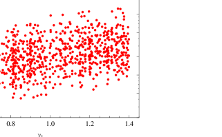
Figure 1: Semilogarithmic plots for $\alpha$ versus $y_{1}$.

In the above numerical results, we have assumed all Yukawa couplings to be $1$. Now let us consider how much the above results change by varying Yukawa couplings. Following the above results, we assume that $|r|\ll 1$ and $ky_{a}={\cal O}(1)$ for $y_{1},y_{2}={\cal O}(1)$. Then, we approximate Eq. (46) as

$$\Delta m_{\mathrm{atm}}^{2}\sim\frac{y_{2}^{4}}{r^{2}}\frac{v^{4}}{M_{1}^{2}}\ ,\qquad\Delta m_{\mathrm{sol}}^{2}\sim-\frac{\sqrt{2}y_{1}y_{2}^{3}}{4y_{a}^{3}k^{3}cs}\frac{v^{4}}{M_{1}^{2}}\ ,\qquad\cot 2\theta_{12}\sim-\frac{y_{2}}{2\sqrt{2}y_{1}y_{a}k}\ .$$ (52)

Hence, the parameters $k$, $r$, and $M_{1}$ are obtained as

$$k\sim\frac{-1}{2\sqrt{2}}\frac{y_{2}}{y_{1}y_{a}}\tan 2\theta_{12}\sim 0.9\times\frac{y_{2}}{y_{1}y_{a}},\qquad r\sim\sqrt{\frac{\Delta m_{\mathrm{sol}}^{2}}{\Delta m_{\mathrm{atm}}^{2}}}\left(\frac{y_{2}}{y_{1}}\right)^{2}\sim 0.2\times\left(\frac{y_{2}}{y_{1}}\right)^{2},$$

$$M_{1}\sim 2\sqrt{2}v^{2}\left(\frac{\cot^{3}2\theta_{12}}{cs\Delta m_{\mathrm{sol}}^{2}}\right)^{1/2}y_{1}^{2}\sim 3\times 10^{15}\times y_{1}^{2}{\rm~{}~{}GeV},$$ (53)

which leads to

$$\alpha=\frac{M_{1}k}{\Lambda}\sim 0.001\times\frac{y_{1}y_{2}}{y_{a}}.$$ (54)

The ratio $y_{2}/y_{1}$ must be of ${\cal O}(1)$ in order that the above approximation is valid, i.e. $y_{a}k={\cal O}(1)$. Thus, values of $k$, $r$ and $M_{1}$ are of the same order as those in Eq. (48). However, the value of $\alpha$ would change its order in some region even if we vary $y_{1},y_{2}$ and $y_{a}$ by ${\cal O}(1)$, because $\alpha$ depends basically on a cube of ${\cal O}(1)$ parameters, i.e. $2^{3}\sim 10$ and $0.5^{3}\sim 0.1$. Let us investigate this behavior numerically. We use Eq. (46) and vary $y_{1}$, $y_{2}$, and $y_{a}$ in the range of $0.5-1.4$ and taking account for the $3\sigma$ error-bar of input experimental data $\Delta m^{2}_{\rm atm}$, $\Delta m^{2}_{\rm sol}$, and $\theta_{12}$. We show the random plots of $\alpha$ versus $y_{1}$ in Fig. 1. It is found that the value of $\alpha$ is predicted around $10^{-4}-10^{-2}$. The dependences of the value of $\alpha$ on other Yukawa couplings such as $y_{2}$ and $y_{a}$ are similar to the case of $y_{1}$. Thus we obtain small $\alpha$ as long as Yukawa couplings are of ${\cal O}(1)$.

4 Summary and Discussion

We have presented the $D_{4}\times Z_{2}$ flavor symmetry, which is different from the previous work by Grimus and Lavoura. Our model has one Higgs doublet although the neutrino mass matrix has the same structure as the one in the model by Grimus and Lavoura. Our model reduces to the standard model in the low energy and there is no FCNC at the tree level.

In order to realize the tri-bimaximal mixing, the condition $\cot 2\theta_{12}=\frac{1}{2\sqrt{2}}$ must be satisfied. Then, we have the condition $y_{1}^{2}r-y_{2}^{2}=y_{1}y_{2}y_{a}k$. Taking Yukawa couplings to be order one, this condition turns to simple one $r\simeq k+1$, which is easily realized by adjusting parameters in our model.

It would be interesting to study supersymmetric extension of our model. In such a supersymmetric $D_{4}$ model, we would have a specific pattern of superpartner mass matrices. We would study it in a separate paper [10].

Finally, we comment on the possibility for stringy realization of our model. The $D_{4}$ flavor symmetry can be derived e.g. from heterotic string models on factorizable orbifolds including the $Z_{2}$ orbifold like $Z_{2}\times Z_{M}$ orbifolds [5, 6]. Indeed, several semi-realistic models have been constructed with three families [5, 7], where three families consist of $D_{4}$ trivial singlets and doublets. From this viewpoint, our $D_{4}$ flavor structure would be natural. However, such orbifold models include only $D_{4}$ trivial singlets and doublets, but not $D_{4}$ non-trivial singlets as fundamental states. The $D_{4}$ non-trivial singlet $\chi_{-+}$ plays an important role in our model. We need to assume that $\chi_{-+}$ is a composite scalar of doublets, in order to obtain $\chi_{-+}$ from the $Z_{2}$ orbifold. Another possibility would be factorizable heterotic orbifold models including the $Z_{4}$ orbifold like $Z_{4}\times Z_{M}$ orbifolds, because such orbifold models can lead to the $D_{4}$ flavor symmetry, where non-trivial singlets as well as trivial singlets and doublets can appear as fundamental modes [6]. Thus, it would be interesting to consider the realization of our $D_{4}$ model from $Z_{4}$ orbifold models.

References

- [1] M. Maltoni, T. Schwetz, M. Tortola, and J.W.F. Valle, New J. Phys. 6, 122 (2004).
- [2] G.L. Fogli, E. Lisi, A. Marrone, and A. Palazzo, Prog. Part. Nucl. Phys. 57, 742 (2006).
-
[3]
P.F. Harrison, D.H. Perkins, and W.G. Scott,
Phys. Lett. B 530, 167 (2002);
P.F. Harrison and W.G. Scott, Phys. Lett. B 535, 163 (2002). -
[4]
See for review, e.g.
E. Ma, arXiv:hep-ph/0612013 (2006); arXiv:0705.0327 (2007) and references therein. - [5] T. Kobayashi, S. Raby and R. J. Zhang, Nucl. Phys. B 704, 3 (2005).
- [6] T. Kobayashi, H. P. Nilles, F. Ploger, S. Raby and M. Ratz, Nucl. Phys. B 768, 135 (2007).
-
[7]
T. Kobayashi, S. Raby and R. J. Zhang,
Phys. Lett. B 593, 262 (2004);
W. Buchmuller, K. Hamaguchi, O. Lebedev and M. Ratz, Nucl. Phys. B 785, 149 (2007);
O. Lebedev, H. P. Nilles, S. Raby, S. Ramos-Sanchez, M. Ratz, P. K. S. Vaudrevange and A. Wingerter, Phys. Lett. B 645, 88 (2007). - [8] W. Grimus and L. Lavoura, Phys. Lett. B 572, 189 (2003).
-
[9]
W. Grimus, A. S. Joshipura, S. Kaneko, L. Lavoura, and M. Tanimoto,
JHEP 0407 078 (2004);
W. Grimus, A. S. Joshipura, S. Kaneko, L. Lavoura, H. Sawanaka, and M. Tanimoto, Nucl. Phys. B 713 151 (2005);
P. Ko, T. Kobayashi, J. h. Park and S. Raby, Phys. Rev. D 76, 035005 (2007) [Erratum-ibid. D 76, 059901 (2007)];
A. Blum, R.N. Mohapatra, and W. Rodejohann, Phys. Rev. D 76 053003 (2007);
A. Blum, C. Hagedorn, and M. Lindner, arXiv:0709.3450. - [10] H. Ishimori, T. Kobayashi, H. Ohki, Y. Omura, R. Takahashi, M. Tanimoto, in preparation.