The RR Lyrae Period-Luminosity-(Pseudo-)Color and Period-Color-(Pseudo-)Color Relations in the Strömgren Photometric System: Theoretical Calibration

Abstract

We present a theoretical calibration of the RR Lyrae period-luminosity-color and period-color-color relations in the multiband uvby Strömgren photometric system. Our theoretical work is based on calculations of synthetic horizontal branches (HBs) for four different metallicities, fully taking into account evolutionary effects for a wide range in metallicities and HB morphologies. While our results show that “pure” period-luminosity and period-color relations do not exist in the Strömgren system, which is due to the large scatter that is brought about by evolutionary effects when the $uvby$ bandpasses are used, they also reveal that such scatter can be almost completely taken into account by incorporating Strömgren pseudo-color [$C_{0}\equiv(u\!-\!v)_{0}-(v\!-\!b)_{0}$] terms into those equations, thus leading to tight period-luminosity-pseudo-color (PLpsC) and period-color-pseudo-color (PCpsC) relations. We provide the latter in the form of analytical fits, so that they can be applied with high precision even in the case of field stars. In view of the very small sensitivity of $C_{0}$ to interstellar reddening, our PLpsC and PCpsC relations should be especially useful for the derivation of high-precision distance and reddening values. In this sense, we carry out a first application of our relations to field RR Lyrae stars, finding evidence that the stars RR Lyr, SU Dra, and SS Leo – but not SV Hya – are somewhat overluminous (by amounts ranging from $\simeq 0.05$ to 0.20 mag in $y$, and thus $V$) with respect to the average for other RR Lyrae stars of similar metallicity.

1. Introduction

Due to the special characteritics of the Strömgren (1963) $uvby$ passband system, it represents an invaluable tool in the study of the physical parameters of stars, such as effective temperature, surface gravity, metallicity, and even age (e.g., Schuster & Nissen, 1989; Grundahl et al., 2000). More recently, it has also been shown that this system – and its u passband in particular – provides us with a sensitive diagnostic of radiative levitation and gravitational settling phenomena taking place in hot horizontal branch (HB) stars (Grundahl et al., 1999). While observations in this system have traditionally been limited to bright and nearby stellar systems, over the past decade and a half, with the advent of modern CCD detectors and increasingly large collector areas, the range of systems within reach of observations in the uvby passband has been increasing dramatically, thus giving a renewed impetus for astrophysical applications of $uvby$ observations. Accordingly, the main purpose of the present paper is to present the first extensive theoretical calibration of the RR Lyrae (RRL) period-luminosity-color and period-color-color relationships in the Strömgren system, thus enabling the latter’s use for distance and reddening determinations throughout the old components of the Local Group.

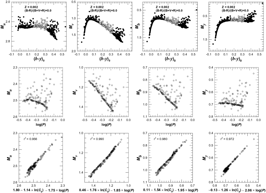
Figure 1.— Upper panels: Morphology of the HB in the CMD when different Strömgren bandpasses (from left to right, $u$, $v$, $b$, $y$) are used, based on synthetic calculations. RRL variables are shown as open circles, and non-variable stars as black circles. Middle panels: Corresponding distributions in the absolute magnitude–log-period (or PL) plane. Lower panels: Corresponding RRL distributions in the absolute magnitude–log-period–(pseudo-)color plane. Note the dramatic reduction in scatter that is brought about with the inclusion of a $C_{0}$-dependent term (the correlation coefficient $r$ is shown in the lower panels). All plots refer to an HB simulation with $Z=0.002$ and an intermediate HB type, as indicated in the upper panels.

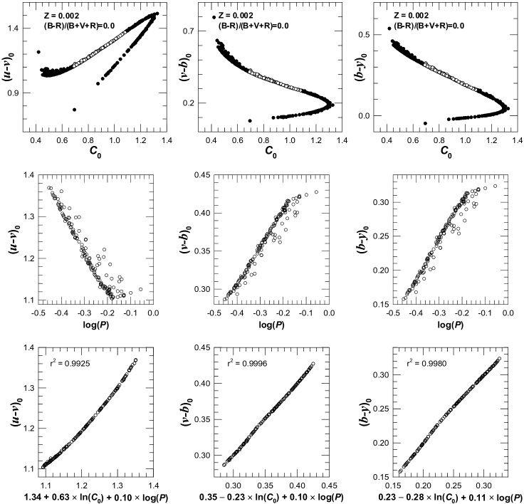
Figure 2.— Upper panels: Morphology of the HB in the color-pseudo color plane when different Strömgren-based colors are used [left: $(u\!-\!v)_{0}$; middle: $(v\!-\!b)_{0}$; right: $(b\!-\!y)_{0}$], based on synthetic calculations. RRL variables are shown as open circles, and non-variable stars as black circles. Middle panels: Corresponding distributions in the color–log-period (or PC) plane. Lower panels: Corresponding RRL distributions in the color–log-period–(pseudo-)color plane. Note the dramatic reduction in scatter that is brought about with the inclusion of a $C_{0}$-dependent term (the correlation coefficient $r$ is shown in the lower panels). All plots refer to an HB simulation with $Z=0.002$ and an intermediate HB type, as indicated in the upper panels.

HB stars form a prop to estimate parameters in globular clusters (GC) and nearby galaxies, including their distance, age, and chemical composition. RRL variables, in particular, as the cornerstone of the Population II distance scale, can help us determine the distances to old and sufficiently metal-poor systems, in which this type of variable star is commonly found in large numbers. RRL stars are radially pulsating variable stars with periods in the range between about 0.2 d and 1.0 d, and they are abundantly present in GCs and the dwarf galaxies in the neighborhood of the Milky Way (e.g., Catelan, 2004, 2005, and references therein). RRL stars have also been positively identified in the M31 field (e.g., Brown et al., 2004; Dolphin et al., 2004) and in some of Andromeda’s companions (e.g., Pritzl et al., 2005a), and in at least four M31 globular clusters (Clementini et al., 2001).

While period-luminosity (PL) relations in the near-infrared bandpasses have been known and studied for a long time now (e.g., Longmore, Fernley, & Jameson, 1986; Bono et al., 2001; Catelan, Pritzl, & Smith, 2004; Del Principe et al., 2006), to the best of our knowledge no such studies have ever been carried out in the Strömgren (1963) passband system, perhaps in view of the fact that the latter does not contain any bandpasses in the near infrared, and indeed in the Johnson-Cousins system there are no good PL relations in the visual, except perhaps in $I$ (Catelan et al., 2004). However, given that the Strömgren (1963) has already proved superior to the wide-band Johnson-Cousins system in deriving stellar physical parameters, it seemed to us well worth the while to carry out a theoretical investigation of the PL (and period-color, or PC) relation in this system. Accordingly, we have carried out, on the basis of evolutionary models and HB simulations, the first analysis of the subject, discovering the presence of tight PL-pseudo-color (PLpsC) and PC-pseudo-color (PCpsC) relations for RRL stars – where the pseudo-color is defined as $C_{0}\equiv(u\!-\!v)_{0}-(v\!-\!b)_{0}$, and is well known to be quite insensitive to reddening (e.g., Crawford & Mandwewala, 1976).

We begin by presenting, in §2, the theoretical framework upon which our study is based. In §3, we explain the origin of the derived PLpsC and PCpsC relations in the Strömgren system. In §4 we provide the first calibration of the RRL PLpsC and PCpsC relations. §5 presents some comments and warnings regarding the application of these relations to the analysis of empirical data. A first comparison with the observations is presented in §6. Finally, some concluding remarks are provided in §7.

2. Models

The HB simulations computed in the present paper are similar to those described in Catelan (2004) and Catelan et al. (2004), to which the reader is referred for further details and references about the HB synthesis method. Catelan et al. argue that these models are consistent with a distance modulus to the Large Magellanic Cloud of $(m\!-\!M)_{0}=18.47$ mag. Note, however, that this value is based on the empirical prescriptions for the LMC by Gratton et al. (2004); using the independent measurements by Borissova et al. (2004), a distance modulus of $(m\!-\!M)_{0}=18.50$ mag would derive instead.

As in Catelan et al. (2004), we employed four sets of evolutionary tracks to compute our HB simulations. These tracks were computed by Catelan et al. (1998) for $Z=0.0005$ and $Z=0.0010$, and by Sweigart & Catelan (1998) for $Z=0.0020$ and $Z=0.0060$. The evolutionary tracks assume a main-sequence helium abundance of $Y_{\rm MS}=23\%$ by mass and scaled-solar compositions. Helium-enhanced tracks were also computed. The mass distribution along the HB in our simulations is represented by a normal deviate with a mass dispersion $\sigma_{M}=0.02\,M_{\odot}$. In the present paper, we have incorporated color transformation and bolometric correction tables for the uvby system, as provided by Clem et al. (2004), to carry out the transformations from the theoretical $(\log L,\log T_{\rm eff})$ plane to the empirical ones. Those tables include the relevant ranges of effective temperature and surface gravities for HB stars, thus being clearly adequate for RRL work. We warn the reader that the quoted bolometric corrections, over the full range of interest for RRL work, differ systematically (${\rm BC}_{y}={\rm BC}_{V}+0.03$) from those adopted in Catelan et al. (2004), which in turn came from VandenBerg (1999, priv. comm.). This is likely due to a different bolometric correction for the Sun, as adopted in the VandenBerg and in the Clem et al. studies. Therefore, when compared with the Catelan et al. (2004) $V$-band magnitudes, the present $y$-band magnitudes are, for the same gravity and temperature combination, 0.03 mag brighter. This also implies distances to the LMC that are correspondingly longer, compared to Catelan et al. (2004) (see §4.2 below).

To define the blue edge of the instability strip, we use equation (1) in Caputo et al. (1987), but applying a shift by $-200$ K to the temperature values thus derived. The width of the instability strip has been taken as $\Delta\log T_{\rm eff}=0.075$; this provides the temperature of the red edge of the instability strip for each star once its blue edge has been determined. These choices provide a good agreement with more recent theoretical prescriptions and the observations (see §6 in Catelan, 2004, for a detailed discussion).

We include both RRab (also classified as RR0) and RRc (RR1) variables in our synthetic PLpsC and PCpsC relations. The computed periods for those stars are based on equation (4) in Caputo et al. (1998). Therefore, to compare our model prescriptions with the observations, the observed RRc periods must be “fundamentalized” by adding 0.128 to the logarithm of the period.

3. Genesis of the RRL PLpsC and PCpsC Relations

In Figures 1 and 2, we show results for an HB simulation computed for $Y_{\rm MS}=23\%$ and a metallicity $Z=0.002$, and an intermediate HB morphology, as indicated by a value of the Lee-Zinn parameter $\mathcal{L}\equiv\mathcal{(B-R)/(B+V+R)}=0.0$ (where $\mathcal{B,R,V}$ represent the numbers of blue, red, and variable – RRL-type – HB stars, respectively). In the upper row of Figure 1, from left to right, one finds the resulting color-magnitude diagrams (CMDs) in the $[M_{u},\,(b\!-\!y)_{0}$], $[M_{v},\,(b\!-\!y)_{0}$], $[M_{b},\,(b\!-\!y)_{0}$], and $[M_{y},\,(b\!-\!y)_{0}]$ planes, respectively, whereas the middle and bottom rows show the resulting PL and (simple, log-linear) PLpsC relations. In the upper row of Figure 2, on the other hand, one finds the resulting $[(u\!-\!v)_{0},C_{0}]$, $[(v\!-\!b)_{0},C_{0}]$, and $[(b\!-\!y)_{0},C_{0}]$ color-(pseudo-) color diagrams, whereas the middle and bottom rows of the same figure show the resulting period-color and (simple, log-linear) PCpsC relations.

In the Strömgren system, the magnitudes in the y passband are required to closely match those in the $V$ passband of the Johnson-Cousins system, which is why the CMD in the upper right panel of Figure 1 appears so similar to those routinely derived in the latter system. Such a similarity also allows us to compare our simulations with Catelan et al. (2004), since the latter have shown that the flatness of the HB in their $V$-band simulations impacts directly the corresponding PL relation. Indeed, as was the case in $V$, the horizontal nature of the $M_{y},\,(b\!-\!y)_{0}$ CMD also leads to an essentially flat PL relation in $M_{y}$, with much scatter as a consequence of evolutionary effects. In like vein, the bluer Strömgren passbands show a behavior totally analogous to that described in Catelan et al. (2004) for the bluer $UB$ passbands of the Johnson-Cousins system: as can be seen from Figure 1, the effects of luminosity and temperature variations are nearly orthogonal in the period-absolute magnitude plane, which leads to large amounts of scatter in the corresponding PL relations.

In this sense, Catelan et al. (2004) have pointed out that such scatter is so large in the $UBV$ passbands as to virtually render the corresponding PL relations useless, as opposed to what happens for redder passbands where the effects of temperature and luminosity variations become increasingly parallel in the period-absolute magnitude plane. As a consequence, increasingly tight, and therefore useful, PL relations obtain towards the near-infrared. In the Strömgren system, on the other hand, near-infrared bandpasses are lacking, so that one must resort to a different strategy in order to obtain useful relationships involving the pulsation period and the absolute magnitude in this filter system.

In this sense, our simulations reveal that, if a pseudo-color $C_{0}$ term is added to the PL relations, the scatter essentially disappears (see the bottom row in Fig. 1). This is especially encouraging in view of the fact that the pseudo-color $C_{0}$ of the Strömgren system is barely affected by reddening (e.g., Crawford & Mandwewala, 1976), thus being very close to its uncorrected value, $C_{1}\equiv(u\!-\!v)-(v\!-\!b)$. Quantitatively, one finds $C_{0}=C_{1}-0.15\,E(\bv)$. As a consequence, calibrated PLpsC relationships in which this pseudo-color index is used are expected to provide us with very useful tools to derive the distances to RRL-rich stellar systems, and even to individual (e.g., field) RRL stars.

In like vein, the bottom row of Figure 2 reveals that, by adding in a pseudo-color term, one is also able to reduce dramatically the scatter that was present in the original period-color relations (middle row in Fig. 2). Accordingly, our resulting PCpsC relationships are also expected to allow one to determine the reddenings of the systems to which the RRL belong, based only on the observed periods, (reddening-insensitive) pseudo-colors, and the reddened colors of individual RRL stars.

4. The RRL PLpsC and PCpsC Relations Calibrated

We have computed, for each of the four metallicity values indicated in §2 and a $Y_{\rm MS}=23\%$, extensive sequences of HB simulations that produce from very blue to very red HB types. These simulations do not include such effects as HB bimodality or the impact of second parameters other than age or mass loss on the red giant branch (but see §4.1 below for the effects of an increase in the helium abundance).

The whole set of simulations contains a total of 336,576 synthetic RRL stars with metallicities ranging from $Z=0.0005$ to $0.006$ and HB morphologies from $\mathcal{L}=-0.95$ to +0.95. As in Catelan & Cortés (2008), we find that, for each individual metallicity, the derived Strömgren magnitudes are well described by analytical fits that involve up to cubic terms in (the log of) $C_{0}$, whereas a linear term in $\log P$ suffices. Rather than providing the forms of these relations for each metallicity separately (see Catelan & Cortés, 2008, for the $Z=0.002$ case), we have here attempted to obtain fits in which all metallicities are simultaneously taken into account. This was accomplished by adopting a simple quadratic dependence on metallicity for each of the coefficients in the original fit. Here we provide fits for Strömgren $y$ and for the colors $b-y$, $v-b$, and $u-v$, from which the individual magnitudes in $u$, $v$, $b$ can be straightforwardly computed.

The final relations that we obtained are thus of the form:

$${\rm mag\,\,or\,\,color}=\sum_{i=0}^{2}a_{i}(\log Z)^{i} + \sum_{i=0}^{2}b_{i}(\log Z)^{i}(\ln C_{0})$$ (1)

$$+ \sum_{i=0}^{2}c_{i}(\log Z)^{i}(\ln C_{0})^{2}$$

$$+ \sum_{i=0}^{2}d_{i}(\log Z)^{i}(\ln C_{0})^{3}$$

$$+ e_{0}(\log P),$$

where “mag” stands for the absolute magnitude in $y$, whereas “color” represents any of the colors $b-y$, $v-b$, and $u-v$. In this expression, $C_{0}$ is the Strömgren system’s pseudo-color, and $P$ is the fundamental RRL period (in days). The corresponding coefficients, along with their errors, are given in Table 1. (Naturally, the $c_{0}$ coefficient that appears in this table is not the same as the Strömgren pseudo-color $C_{0}$, which is given in capital letters throughout this paper to avoid confusion.)

Table 1Coefficients of the Fits

Coefficient	Value	Error		Coefficient	Value	Error
$y$				$b-y$
$a_{0}$	$+0.0895$	$0.0052$		$a_{0}$	$+0.2440$	$0.0005$
$a_{1}$	$+0.0037$	$0.0037$		$a_{1}$	$+0.0044$	$0.0004$
$a_{2}$	$-0.0252$	$0.0007$		$a_{2}$	$-0.0002$	$0.0001$
$b_{0}$	$-0.5242$	$0.0766$		$b_{0}$	$-0.5472$	$0.0076$
$b_{1}$	$+0.6885$	$0.0564$		$b_{1}$	$-0.1280$	$0.0056$
$b_{2}$	$+0.1458$	$0.0102$		$b_{2}$	$-0.0164$	$0.0010$
$c_{0}$	$+3.2354$	$0.6837$		$c_{0}$	$-2.3427$	$0.0682$
$c_{1}$	$+3.0981$	$0.4920$		$c_{1}$	$-1.6363$	$0.0491$
$c_{2}$	$+0.6059$	$0.0874$		$c_{2}$	$-0.3065$	$0.0087$
$d_{0}$	$-11.7261$	$1.5383$		$d_{0}$	$-8.4066$	$0.1534$
$d_{1}$	$-5.5043$	$1.0822$		$d_{1}$	$-5.7964$	$0.1079$
$d_{2}$	$-0.6123$	$0.1885$		$d_{2}$	$-1.0051$	$0.0188$
$e_{0}$	$-2.0066$	$0.0015$		$e_{0}$	$+0.1044$	$0.0001$
$v-b$				$u-v$
$a_{0}$	$+0.5569$	$0.0007$		$a_{0}$	$+1.5574$	$0.0007$
$a_{1}$	$+0.1121$	$0.0005$		$a_{1}$	$+0.1124$	$0.0005$
$a_{2}$	$+0.0124$	$0.0001$		$a_{2}$	$+0.0125$	$0.0001$
$b_{0}$	$-0.5220$	$0.0103$		$b_{0}$	$+0.4855$	$0.0104$
$b_{1}$	$-0.1267$	$0.0076$		$b_{1}$	$-0.1215$	$0.0077$
$b_{2}$	$-0.0087$	$0.0014$		$b_{2}$	$-0.0078$	$0.0014$
$c_{0}$	$-1.5715$	$0.0918$		$c_{0}$	$-1.0571$	$0.0930$
$c_{1}$	$-1.0406$	$0.0661$		$c_{1}$	$-1.0305$	$0.0669$
$c_{2}$	$-0.1842$	$0.0117$		$c_{2}$	$-0.1830$	$0.0119$
$d_{0}$	$-7.6106$	$0.2067$		$d_{0}$	$-7.4495$	$0.2093$
$d_{1}$	$-4.8869$	$0.1454$		$d_{1}$	$-4.8832$	$0.1472$
$d_{2}$	$-0.7979$	$0.0253$		$d_{2}$	$-0.7988$	$0.0256$
$e_{0}$	$+0.0882$	$0.0002$		$e_{0}$	$+0.0884$	$0.0002$

Table 2Analytical Fits: Quality Diagnostics

Fit	$r$	std. error
$y$	$+0.9978$	$0.0084$
$b-y$	$+0.9998$	$0.0008$
$v-b$	$+0.9996$	$0.0011$
$u-v$	$+0.9999$	$0.0011$

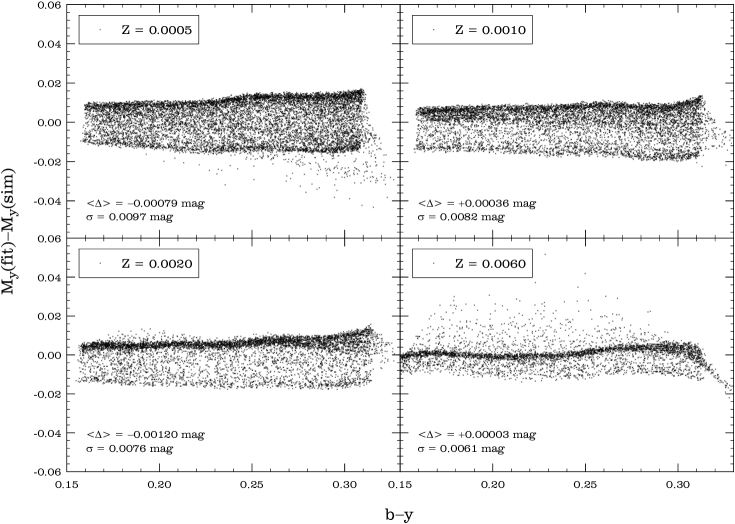
Figure 3.— Difference between the absolute magnitude in $y$, as predicted by equation (1), and its input value (from the HB simulations), plotted as a function of the $b-y$ color (from the same simulations) for four different metallicities: $Z=0.0005$ (upper left), 0.001 (upper right), 0.002 (lower left), 0.006 (lower right). A total of 28,992 randomly selected synthetic stars is shown for all metallicities. The average magnitude difference is indicated in the lower left corner of each panel, along with the corresponding standard deviation. The latter is a direct indicator of the precision with which equation (1) is able to provide the $M_{y}$ values. Note, accordingly, that for all metallicities equation (1) yields $M_{y}$ values with a precision better than 0.01 mag.

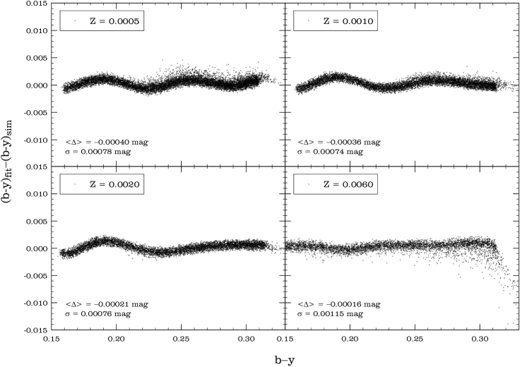
Figure 4.— As in Figure 3, but for $b-y$. Note that the precision in the $b-y$ colors provided by equation (1) is at the mmag level.

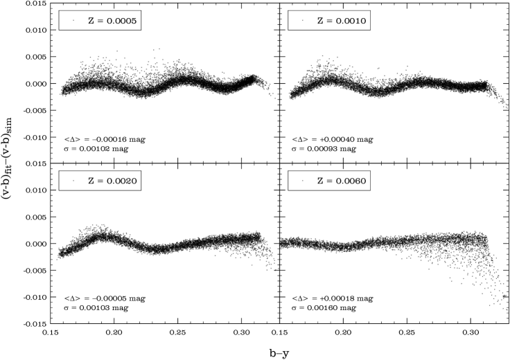
Figure 5.— As in Figure 3, but for $v-b$. Note that the precision in the $v-b$ colors provided by equation (1) is at the mmag level.

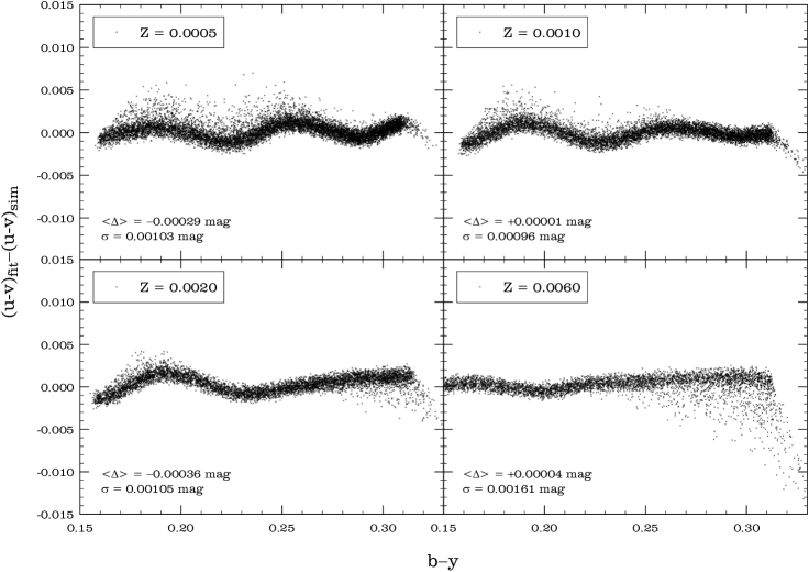
Figure 6.— As in Figure 3, but for $u-v$. Note that the precision in the $u-v$ colors provided by equation (1) is at the mmag level.

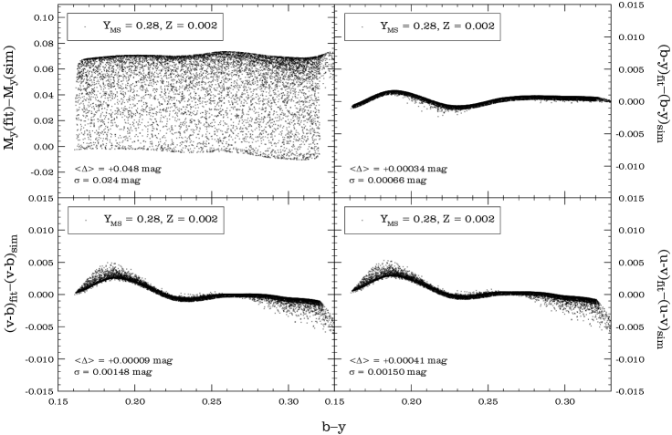
Figure 7.— Effect of an increase in the helium abundance upon the derived relations. Here we give the difference between the quantities predicted by equation (1) and its input value from HB simulations computed for a $Y_{\rm MS}=0.28$ and $Z=0.002$. Upper left: $M_{y}$; upper right: $b-y$; lower left: $v-b$; lower right: $u-v$. All quantities are plotted as a function of the $b-y$ value from the simulations. A total of 8338 synthetic stars is shown in each panel. As can be seen, an increased helium has a clear influence upon the absolute magnitudes, but not so upon the derived colors.

We stress that these equations are able to reproduce the input values (from the HB simulations) with remarkable precision. This is shown in Table 2, where the correlation coefficient $r$ and the standard error of the estimate are given for each of the four equations. We also show, in Figures 3, 4, 5, and 6, the residuals [in the sense eq. (1) minus input values (from the simulations)] for a random subset of 28,992 synthetic stars drawn from the original pool of 336,576 synthetic RRL stars in the HB simulations, for the fits computed for $y$, $b-y$, $v-b$, and $u-v$, respectively. These plots further illustrate that the Strömgren magnitudes and colors can be predicted from the data provided in equation (1) and Table 1 with great precision.

Finally, we note that equation (1) can be trivially expressed in terms of [Fe/H]; this can be accomplished using the relation

$$\log Z={\rm[M/H]}-1.765,$$ (2)

which is the same as equation (9) in Catelan et al. (2004). In this sense, the effects of an enhancement in $\alpha$-capture elements with respect to a solar-scaled mixture, such as observed amongst Galactic halo stars (e.g., Pritzl, Venn, & Irwin, 2005b, and references therein), can be taken into account by using the following scaling relation (Salaris, Chieffi, & Straniero, 1993):

$${\rm[M/H]}={\rm[Fe/H]}+\log(0.638\,f+0.362),$$ (3)

where $f=10^{\rm[\alpha/Fe]}$. However, such a relation should be used with due care for metallicities $Z>0.003$ (VandenBerg et al., 2000).

4.1. The Effect of Helium Abundance

As already stated (§2), the aforementioned simulations are based on a fixed mass dispersion ($\sigma_{M}=0.020\,M_{\odot}$) and helium abundance (23%). However, several authors have pointed out that old, helium-enhanced populations may exist, even at low metallicities, thus opening the possibility that helium-enhanced RRL stars may also exist (see Catelan, 2005, for a review). How would a helium enhancement affect the derived relations for RRL stars?

In order to answer this question, we have computed additional sets of synthetic HBs for a $Y_{\rm MS}=28\%$ ($Z=0.0020$), and applied the same relations as in equation (1) to check how much we would err by assuming that the relations derived for a $Y_{\rm MS}=23\%$ are valid also for a higher $Y$. The enhanced-$Y$ simulations cover the full range of HB types, from very blue to very red, and include a total of 8338 synthetic RRL stars.

The residuals, in the sense equation (1) minus simulations, are shown in Figure 7. In this figure, the upper left panel shows the residuals for $M_{y}$, the upper right one for $b-y$, the lower left one for $v-b$, and the lower right one for $u-v$. As in the previous figures, the average residual and standard deviation are also provided in the insets.

It is immediately apparent that our derived relations for $b-y$, $v-b$, and $u-v$ can be safely applied to RRL stars with a significantly enhanced helium content, the implied errors being significantly smaller than 0.01 mag. In the case of $M_{y}$, there is a clear offset in the zero point, as well as an increased dispersion in comparison with Figure 3. Still, the standard deviation remains a modest $0.024$ mag, and the full dispersion range is of order 0.08 mag only – to be compared with the actual dispersion in $M_{y}$ magnitudes from the HB simulations in the enhanced-$Y$ case, which amounts to a full 0.59 mag (i.e., $M_{y}$ values for individual RRL stars range from 0.58 mag at their faintest to $-0.01$ mag at their brightest). Therefore, if a correction to the zero point $a_{0}$ for $M_{y}$ in Table 1 by $dM_{y}/dY=-0.048/(0.28-0.23)=-0.96$ (i.e., in the sense that eq. 1 predicts too faint magnitudes) is duly taken into account, equation (1) can also be used to provide useful information on the absolute magnitudes of RRL stars with enhanced helium abundances.

To close, we note that, as in Catelan et al. (2004), we have also checked the effect of changing the mass dispersion $\sigma_{M}$ upon our results, and found that equation (1) adequately covers the possibility of different $\sigma_{M}$ values.

4.2. Average Relations for $M_{y}$

It is common practice, in RRL work, to employ a simple, linear relation between average absolute magnitude in the visual and [Fe/H] (e.g., Catelan, 2005, and references therein). On the basis of our models, we find the following relation:

$$M_{y}=(1.4350\pm 0.0009)+(0.2800\pm 0.0003)\,\log Z,$$ (4)

with a correlation coefficient $r=0.835$. As shown by several authors, and as also discussed by Catelan et al. (2004), a quadratic relation may be superior to such a simple linear relation; we accordingly obtain:

$$M_{y}=(2.259\pm 0.007) + (0.883\pm 0.005)\,\log Z$$ (5)

$$+ (0.108\pm 0.001)\,(\log Z)^{2},$$

with a correlation coefficient $r=0.843$. (The small errors in the coefficients are a consequence of the large number of synthetic stars used in deriving these relations.) Note that this expression is basically identical to equation (8) in Catelan et al. (2004), which was obtained for the $V$ band following a similar procedure as in the present paper, except that their zero points differ by 0.03 mag (in the sense that eq. 5 provides slightly brighter magnitudes, as expected; see §2). The true distance modulus to the LMC implied by equation (5) is 18.49 mag (using the data for LMC RRL from Gratton et al., 2004) or 18.53 mag (using instead data from Borissova et al., 2004). Such a value is in agreement, within the errors, with the distance modulus recently determined by Catelan & Cortés (2008), who pegged the zero point of their distance scale to RR Lyr’s trigonometric parallax, and found $(m-M)_{0}^{\rm LMC}=18.44\pm 0.11$.

Equations (4) and (5) are shown in Figure 8. Naturally, absolute magnitudes for individual RRL stars, as derived on the basis of either of these equations, will be much less reliable than those based on equation (1), since the latter is the only one that is able to take evolutionary effects into account on a star-by-star basis. We will come back to this point momentarily (see also Catelan & Cortés, 2008).

5. On Applying Our Relations to RRL Stars

When applying our equation (1) in globular cluster work, the metallicity of the cluster will often be known a priori. However, metallicity estimates may also be unavailable, especially when dealing with field RRL stars. Yet, for a reliable application of our relations to field stars, an estimate of their metallicities must be provided.

The Strömgren system itself may again come to our rescue in such a case. In a forthcoming paper, we shall provide a technique to derive metallicities for RRL stars, based on the Strömgren parameters $m_{0}=(v-b)_{0}-(b-y)_{0}$ (also called the Strömgren “metal-line index”; Strömgren 1963) and $C_{0}$. In the meantime, we recall that RRL metallicities can also be obtained on the basis of their $V$-band light curves using Fourier decomposition (e.g., Jurcsik & Kovács, 1996; Jurcsik, 1998; Kovács & Kupi, 2007; Morgan, Wahl, & Wieckhorst, 2007); since the $y$-band magnitudes are very similar to those in the Johnson-Cousins $V$-band, this means that available calibrations of Fourier decomposition parameters as a function of metallicity can be employed in the Strömgren system as well. Naturally, the reader should keep in mind that such calibrations can only be applied to variable stars that do not show the Blazhko (1907) effect. In addition, in Jurcsik & Kovács a deviation parameter $D_{m}$ was defined to measure the degree of reliability of an ab-type RRL light curve for application of the Fourier decomposition method. In particular, when $D_{m}<3$, the physical, chemical, and photometric parameters, as derived from Fourier fits, should be considered more reliable. Unfortunately, high-$S/N$ light curves in the Strömgren system are more difficult to obtain than in the Johnson-Cousins system, due to the fact that in the former case we are dealing with an intermediate-band system. Longer exposure times may accordingly be needed, but care should be taken to keep these exposures sufficiently short that an insignificant fraction of the star’s pulsation period is encompassed by them.

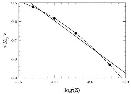
Figure 8.— Correlation between average $M_{y}$ magnitude and metallicity, with equations (4) and (5) (continuous and dashed lines, respectively) overplotted.

The reader should be warned that our relations should be compared against empirical quantities obtained for the so-called equivalent static star. Several procedures have been advanced in the literature for the determination of the latter on the basis of empirically derived magnitudes and colors (e.g., Bono, Caputo, & Stellingwerf, 1995, and references therein). In particular, one should note that, according to the hydrodynamical models provided by Bono et al., one should expect differences between temperatures derived from intensity- or magnitude-averaged colors, on the one hand, and those based on the actual color of the equivalent static star, on the other. As a workaround, these authors set forth very useful amplitude-dependent corrections, which become more important the bluer the bandpass. Unfortunately, to the best of our knowledge a similar study has never been extended to bandpasses bluer than $B$ (but see Bono, Caputo, & Stellingwerf, 1994), as would be required to quantitatively evaluate the impact of nonlinear phenomena upon the derived average quantities using $u$ and $v$ in particular. In this sense, an extension to the Strömgren system of the work that was carried out by Bono et al. in the Johnson-Cousins system would be of great interest. On the other hand, and as noted by the referee, $C_{0}$, being a difference between two colors, is presumably affected to a lesser degree than are the colors themselves (see also Catelan & Cortés, 2008).

Table 3Applications to Field RRL Stars

Star	$P$ (day)	[Fe/H]	$C_{0}$	$(b-y)_{0}$	$(b-y)_{0}$	$\Delta(b-y)_{0}$	$M_{y}$	$M_{y}$	$\Delta M_{y}$
SV Hya	0.479	$-1.10$	0.903	0.212	0.229	0.017	0.680	0.674	$-0.006$
RR Lyr	0.567	$-1.39$	0.853	0.241	0.249	0.008	0.599	0.549	$-0.051$
RR Lyr	0.567	$-1.16$	0.853	0.241	0.252	0.011	0.662	0.587	$-0.075$
SU Dra	0.661	$-1.38$	0.864	0.252	0.256	0.008	0.602	0.402	$-0.200$
SS Leo	0.627	$-1.50$	0.837	0.246	0.257	0.011	0.573	0.463	$-0.111$

As a first, rough approximation to the amplitude-dependent corrections that may be expected in the case of the $(b\!-\!y)_{0}$ color index, Table 4 in Bono et al. (1995), which was computed for the broadband $\bv$ color, may be used as a guide. This table indicates that, except at the very highest amplitudes ($A_{B}>1.8$ mag), the corrections needed to go from the average $\bv$ color (computed directly in intensity or magnitude units) to the color of the equivalent static star are always smaller than 0.025 mag for an ab-type RRL star (a similar limit obtains for RRc stars with amplitudes that are smaller than $A_{B}=1$ mag). It is worth noting, in this sense, that Catelan & Cortés (2008), in their study of the star RR Lyr, have indeed found only small differences between the average magnitudes (including the bluer filters), colors, and $C_{0}$ values, computed following different recipes for finding the properties of the equivalent static star.

Observers are also strongly warned against using single-epoch photometry to derive $C_{1}$ values to be used along with our relations: according to the light curves presented by Siegel (1982), ab-type RRL may present amplitudes in $C_{1}$ that may reach up to 0.6 mag. According to our derived relations, changes in $C_{0}$ by $\pm 0.3$ mag lead to average changes in $M_{y}$ by ${}^{-0.40\pm 0.03}_{+0.61\pm 0.27}$ mag, in $b\!-\!y$ by ${}^{-0.10\pm 0.01}_{+0.11\pm 0.05}$ mag, in $v\!-\!b$ by ${}^{-0.07\pm 0.01}_{+0.12\pm 0.07}$ mag, and in $u\!-\!v$ by ${}^{+0.23\pm 0.01}_{-0.18\pm 0.07}$ mag.

To close, we also note that there do exist some calibrations to derive $T_{\rm eff}$ from $(b\!-\!y)_{0}$, which show that this color is indeed a very good indicator of effective temperature (e.g., Clem et al., 2004). Unfortunately, these calibrations are based on evolutionary states that precede core helium-burning stars. On the other hand, the plane $(b\!-\!y)_{0}-C_{0}$ has been described as a good indicator of effective temperature (and surface gravities) for RRL stars (e.g., Siegel, 1982; McNamara, 1997). Given its tremendous potential, it is very unfortunate that there are not more empirical studies based on Strömgren filters for RRL stars, the papers by Epstein (1969) and Siegel (1982) being notable exceptions.

6. Comparisons with the Observations

While a detailed comparison with the empirical data is beyond the scope of the present paper, in this section we provide a first application of our relations to observations of field RRL stars (see also Catelan & Cortés, 2008). In this sense, Table 3 provides a comparison between colors and magnitudes, as derived from our relations, and (in the case of the $b-y$ colors) those from previous studies (from McNamara, 1997, unless otherwise noted), for stars within the general range of validity of our relations. In column 1, we provide the star’s name; in column 2, the period (in days). The metallicity [Fe/H] is indicated in column 3, whereas column 4 gives the star’s $C_{0}$ value. Column 5 gives the star’s $(b\!-\!y)_{0}$ color from McNamara (1997), whereas column 6 gives the same quantity, as derived from the listed $C_{0}$ and $P$ values on the basis of our equation (1). Column 7 gives the difference between these two color estimates. Column 8 provides $M_{y}$, based on our equation (1), whereas column 9 lists the $M_{y}$ value derived on the basis of equation (5). Column 10 lists the difference between these two $M_{y}$ estimates.

For the star RR Lyr, we provide two different rows, corresponding to two different possibilities for the star’s metallicity value, both based on the Clementini et al. (1995) measurements (which, according to Bragaglia et al. 2001, provide [Fe/H] for the star in the Zinn & West 1984 scale). The global metallicity $Z$ is obtained, on the basis of the indicated [Fe/H] values, using equations (2) and (3). An $\alpha$-enhancement $[\alpha/{\rm Fe}]=+0.31$ (again from Clementini et al., 1995) is assumed for ${\rm[Fe/H]}<-1$, and $[\alpha/{\rm Fe}]=0$ at higher metallicities.

6.1. Colors

Comparing the $(b\!-\!y)_{0}$ colors derived on the basis of our equation (1) with those from McNamara (1997), we find an average difference of $0.011$ mag (in the sense our fit minus McNamara), with standard deviation $0.005$ mag, and a maximum difference of $0.017$ mag (see Table 3). Clearly, our relations provide a very good match to McNamara’s intrinsic color determinations for RRL stars, at least in $(b\!-\!y)$, though a systematic overestimate by $\approx 0.01$ mag cannot be ruled out.

6.2. Absolute Magnitudes

Note that $M_{y}$ values, as derived on the basis of equation (1), do indeed refer to the absolute magnitude of the individual star. $M_{y}$ values derived on the basis of a simple $M_{y}-{\rm[Fe/H]}$ relation such as equation (5), on the other hand, simply provide the average absolute magnitude of RRL stars of metallicity similar to a given star’s. It thus follows that a comparison between these two quantities provides us with a direct estimate of the degree of overluminosity (due to evolutionary effects) in $y$ (and thus similarly in $V$) of individual RRL stars (see also Catelan & Cortés, 2008). This degree of overluminosity is then precisely what the last column of Table 3 provides.

It thus appears that all of the stars that we have studied but one (SV Hya) are somewhat overluminous compared to the expected mean $M_{y}$ for their metallicities. In the case of RR Lyr itself, we find an overluminosity in the range between $0.051-0.075$ mag, depending on the adopted metallicity scale (see Table 3), which is only slightly smaller than the similar result (namely, an overluminosity of $0.077\pm 0.010$ mag in $y$) recently obtained by Catelan & Cortés (2008) on the basis of relations that they derived for $Z=0.002$ models. As pointed out by Catelan & Cortés, due to the fact that empirical versions of our equations (4) and (5) are normally based on the assumption that RR Lyr is representative of the average for its metallicity, a correction to the zero points of these empirical calibrations by this same amount is required (as indeed performed by Catelan & Cortés). This, and again as shown by Catelan & Cortés on the basis of the latest trigonometric parallax values for RR Lyr, leads to a revised true distance modulus for the Large Magellanic Cloud of $(m-M)_{0}=18.44\pm 0.11$ mag.

7. Conclusions

We have presented the first calibration of the RRL PLpsC and PCpsC relations in the uvby bandpasses of the Strömgren system. Though we have shown that “pure” PL and PC relations do not exist in this system due to the scatter brought about by evolutionary effects, we have also demonstrated that the latter can be satisfactorily taken into account by including pseudo-color- (i.e., $C_{0}$-) dependent terms in the calibration – thus leading to our reported period-luminosidy-pseudo-color (PLpsC) and period-color-pseudo-color (PCpsC) relations. The latter are provided in the form of analytical fits (eq. 1 and Table 1), which we show to be able to provide $M_{y}$ values that can be trusted at the $\approx\pm 0.01$ mag level, and $b-y$, $v-b$, and $u-v$ colors that are good at the mmag level. We also show that these relations remain good even in the case of helium-enhanced RRL stars, and provide a helium-dependent correction to the zero point of the relation for $M_{y}$. These relations should be of great help in deriving reddenings and distances to even individual field RRL stars.

By applying our derived relations to a sample of four field RRL stars with Strömgren parameters from the literature (McNamara, 1997), we find evidence that RR Lyr, SU Dra, and SS Leo are overluminous in $y$ (and thus $V$) compared to other stars of similar metallicity, by $0.05-0.08$ mag (depending on the metallicity scale), 0.20 mag, and 0.11 mag, respectively (see also Catelan & Cortés, 2008). SV Hya, on the other hand, appears more representative of the average for its peers, to within 0.01 mag. The fact that we can derive the evolutionary status of even individual field RRL stars using our relations clearly demonstrates the great potential of Strömgren photometry in applications of RRL stars to studies of the Galactic and extragalactic distance scale.

References

- Blazhko (1907) Blazhko, S. 1907, Astron. Nachr., 175, 325
- Bono et al. (1994) Bono, G., Caputo, F., & Stellingwerf, R. F. 1994, ApJ, 432, L51
- Bono et al. (1995) Bono, G., Caputo, F., & Stellingwerf, R. F. 1995, ApJS, 99, 263
- Bono et al. (2001) Bono, G., Caputo, F., Castellani, V., Marconi, M., & Storm, J. 2001, MNRAS, 326, 1183
- Borissova et al. (2004) Borissova, J., Minniti, D., Rejkuba, M., Alves, D., Cook, K. H., & Freeman, K. C. 2004, A&A, 423, 97
- Bragaglia et al. (2001) Bragaglia, A., Gratton, R. G., Carretta, E., Clementini, G., Di Fabrizio, L., & Marconi, M. 2001, AJ, 122, 207
- Brown et al. (2004) Brown, T. M., Ferguson, H., Smith, E., Kimble, R. A., Sweigart, A. V., Renzini, A., & Rich, R. M. 2004, AJ, 127, 2738
- Caputo et al. (1987) Caputo, F., de Stefanis, P., Paez, E., & Quarta, M. L. 1987, A&AS, 68, 119
- Caputo et al. (1998) Caputo, F., Santolamazza, P., & Marconi, M. 1998, MNRAS, 293, 364
- Carretta & Gratton (1997) Carretta, E., & Gratton, R. 1997, A&AS, 121, 95
- Catelan (2004) Catelan, M. 2004, ApJ, 600, 409
- Catelan (2005) Catelan, M. 2005, preprint (astro-ph/0507464)
- Catelan et al. (1998) Catelan, M., Borissova, J., Sweigart, A. V., & Spassova, N. 1998, ApJ, 494, 265
- Catelan & Cortés (2008) Catelan, M., & Cortés, C. 2008, ApJ, in press (astro-ph/0802.2063)
- Catelan et al. (2004) Catelan, M., Pritzl, B. J., & Smith, H. A. 2004, ApJS, 154, 633
- Clem et al. (2004) Clem, J. L., VandenBerg, D. A., Grundahl, F., & Bell, R. A. 2004, AJ, 127, 1227
- Clementini et al. (1995) Clementini, G., Carretta, E., Gratton, R., Merighi, R., Mould, J. R., & McCarthy, J. K. 1995, AJ, 110, 2319
- Clementini et al. (2001) Clementini, G., Federici, L., Corsi, C., Cacciari, C., Bellazzini, M., & Smith, H. A. 2001, ApJ, 559, L109
- Crawford & Mandwewala (1976) Crawford, D. L., & Mandwewala, N. 1976, PASP, 88, 917
- Del Principe et al. (2006) Del Principe, M., et al. 2006, ApJ, 652, 362
- Dolphin et al. (2004) Dolphin, A. E., Saha, A., Olszewski, E. W., Thim, F., Skillman, E. D., Gallagher, J. S., & Hoessel, J. 2004, AJ, 127, 875
- Epstein (1969) Epstein, I. 1969, AJ, 74, 1131
- Gratton et al. (2004) Gratton, R. G., Bragaglia, A., Clementini, G., Carretta, E., Di Fabrizio, L., Maio, M., & Taribello, E. 2004, A&A, 421, 937
- Grundahl et al. (1999) Grundahl, F., Catelan, M., Landsman, W. B., Stetson, P. B., & Andersen, M. I. 1999, ApJ, 524, 242
- Grundahl et al. (2000) Grundahl, F., VandenBerg, D. A., Bell, R. A., Andersen, M. I., & Stetson, P. B. 2000, AJ, 120, 1884
- Jones et al. (1987) Jones, R. V., Carney, B. W., Latham, D. W., & Kurucz, R. L. 1987, ApJ, 312, 254
- Jurcsik (1998) Jurcsik, J. 1998, A&A, 333, 571
- Jurcsik & Kovács (1996) Jurcsik, J., & Kovács, G. 1996, A&A, 312, 111
- Kovács & Kupi (2007) Kovács, G., & Kupi, G. 2007, A&A, 462, 1007
- Longmore et al. (1986) Longmore, A. J., Fernley, J. A., & Jameson, R. F. 1986, MNRAS, 220, 279
- McNamara (1997) McNamara, D. H. 1997, PASP, 109, 857
- Morgan et al. (2007) Morgan, S. M., Wahl, J. N., & Wieckhorst, R. M. 2007, MNRAS, 374, 1421
- Pritzl et al. (2005a) Pritzl, B. J., Armandroff, T. E., Jacoby, G. H., & Da Costa, G. S. 2005a, AJ, 129, 2232
- Pritzl et al. (2005b) Pritzl, B. J., Venn, K. A., & Irwin, M. 2005b, AJ, 130, 2140
- Salaris et al. (1993) Salaris, M., Chieffi, A., & Straniero, O. 1993, ApJ, 414, 580
- Schuster & Nissen (1989) Schuster, W. J., & Nissen, P. E. 1989, A&A, 221, 65
- Siegel (1982) Siegel, M. J. 1982, PASP, 94, 1225
- Stellingwerf (1984) Stellingwerf, R. F. 1984, ApJ, 277, 322
- Strömgren (1963) Strömgren, B. 1963, QJRAS, 4, 8
- Sweigart & Catelan (1998) Sweigart, A. V., & Catelan, M. 1998, ApJ, 501, L63
- VandenBerg et al. (2000) VandenBerg, D. A., Swenson, F. J., Rogers, F. J., Iglesias, C. A., & Alexander, D. R. 2000, ApJ, 532, 430
- Zinn & West (1984) Zinn, R., & West, M. J. 1984, ApJS, 55, 45