Mass accretion rates in self-regulated disks of T Tauri stars

Abstract

We have studied numerically the evolution of protostellar disks around intermediate and upper mass T Tauri stars ($0.25~{}M_{\odot}<M_{\ast}<3.0~{}M_{\odot}$) that have formed self-consistently from the collapse of molecular cloud cores. In the T Tauri phase, disks settle into a self-regulated state, with low-amplitude nonaxisymmetric density perturbations persisting for at least several million years. Our main finding is that the global effect of gravitational torques due to these perturbations is to produce disk accretion rates that are of the correct magnitude to explain observed accretion onto T Tauri stars. Our models yield a correlation between accretion rate $\dot{M}$ and stellar mass $M_{\ast}$ that has a best fit $\dot{M}\propto M_{\ast}^{1.7}$, in good agreement with recent observations. We also predict a near-linear correlation between the disk accretion rate and the disk mass.

1. Introduction

Gaseous circumstellar disks are known to extend anywhere from several to perhaps hundreds of AU around T Tauri stars (TTS), due to the detection of millimeter and submillimeter emission from the associated dust (e.g., Beckwith et al., 1990; Andrews & Williams, 2005). It has recently been recognized that such disks also exist around brown dwarfs (BD), with masses as small as $0.01~{}M_{\sun}$, but with comparable disk-to-star mass ratios as found for TTS (Klein et al., 2003; Scholz et al., 2006). Spectroscopic observations demonstrate that BD share similar accretion properties with TTS. In particular, both have a large scatter in the mass accretion rate ($2-3$ orders of magnitude) at a given stellar mass (Scholz & Jayawardhana, 2006) and, when data for BD and TTS are taken together, the accretion rates $\dot{M}$ show a strong direct dependence on stellar masses $M_{\ast}$, with an approximate scaling $\dot{M}\propto M_{\ast}^{2}$ (e.g., Muzerolle et al., 2003, 2005; Mohanty et al., 2005; Natta et al., 2006).

The origin of the above relation is uncertain. Padoan et al. (2005) have argued that this relation is a consequence of Bondi-Hoyle accretion from the large-scale gas distribution in the parent cloud. Such a scenario neglects the importance of disk physics in determining the accretion rate, and also fails to explain the similarity of accretion rates onto TTS located within molecular clouds and H II regions (Hartmann et al., 2006). An alternative idea is that the accretion onto the stellar surface is controlled by viscous disk evolution. Alexander & Armitage (2006) and Hartmann et al. (2006) have invoked different initial input parameters or scaling relations into the standard viscous disk evolution models of Hartmann et al. (1998) in order to explain the approximate $\dot{M}\propto M_{\ast}^{2}$ scaling. These models treat disks as isolated smooth axisymmetric structures that evolve due to an unspecified source of turbulent viscosity that has ad-hoc spatial dependence as well as temporal independence. Dullemond et al. (2006) have taken a more fundamental approach of linking the disk evolution to the properties of the collapsing core from which it forms, but still relies upon the ad-hoc $\alpha$-viscosity prescription to model the angular momentum transport within the disk.

In this Letter, we take the basic approach of studying the mass accretion rate within disks that have formed self-consistently due to the collapse of cloud cores. The disks are actually profoundly nonaxisymmetric when formed in this manner, and experience significant envelope-induced gravitational instability and accretion bursts during their early evolution (Vorobyov & Basu, 2005, 2006, hereafter VB05,VB06, respectively). Here, we explore the late evolution of such self-consistently formed disks, when their evolution is governed by low amplitude nonaxisymmetric density perturbations (Vorobyov & Basu, 2007, hereafter VB07). The gravitational torques produced by these perturbations are sufficient to explain the observed magnitudes and scatter of accretion rates of TTS, and even approximately fit the observed $\dot{M}-M_{\ast}$ relation.

2. Model description

We use the thin-disk approximation to compute the evolution of rotating, gravitationally bound cloud cores. This allows efficient calculation of the long-term evolution of a large number of models. The derivation of the relevant equations, details of the numerical code and tests are given in VB06. The basic equations of mass and momentum transport are

$$\frac{{\partial\Sigma}}{{\partial t}} = -\nabla_{p}\cdot\left(\Sigma\mbox{\boldmath$v$}_{p}\right),$$ (1)

$$\Sigma\frac{d\mbox{\boldmath$v$}_{p}}{dt} = -\nabla_{p}{\cal P}+\Sigma\mbox{\boldmath$g$}_{p}\,,$$ (2)

where $\Sigma$ is the mass surface density, ${\cal P}$ is the vertically integrated gas pressure, $\mbox{\boldmath$v$}_{p}$ is the velocity in the disk plane, $\mbox{\boldmath$g$}_{p}$ is the gravitational acceleration in the disk plane, and $\nabla_{p}$ is the gradient along the planar coordinates of the disk. Equations (1) and (2) are closed with a barotropic equation that makes a transition from isothermal to adiabatic evolution at $\Sigma=\Sigma_{\rm cr}=36.2$ g cm^-2. This approach bypasses the detailed cooling and heating mechanisms, but provides a good fit to the density-temperature relation in collapsing cloud cores (see VB06). In the late phase of disk evolution, the stellar irradiation is expected to be a significant source of heating and is neglected in our simulation. Much of the region of enhanced temperature would fall within our “sink cell” (see below), but our calculated temperatures at $\sim 10$ AU are also somewhat lower than found in models of stellar irradiation onto flared passive disks (Chiang & Goldreich, 1997). Further details of such a comparison are given by VB07.

Equations (1) and (2) are solved in polar coordinates $(r,\phi)$ on a numerical grid with $128\times 128$ points. The radial points are logarithmically spaced. The innermost grid point is located at $r=5$ AU, and the size of the first adjacent cell is 0.3 AU. We introduce a “sink cell” at $r<5$ AU, which represents the central protostar plus some circumstellar disk material, and impose a free inflow inner boundary condition. The outer boundary is such that the cloud has a constant mass and volume.

The gas has a mean molecular mass $2.33\,m_{\rm H}$ and is initially isothermal with temperature $T$ ($=10$ K) and isothermal sound speed $c_{\rm s}$. The initial distributions of $\Sigma$ and angular velocity $\Omega$ are those characteristic of a collapsing axisymmetric magnetically supercritical core (Basu, 1997):

$$\Sigma={r_{0}\Sigma_{0}\over\sqrt{r^{2}+r_{0}^{2}}}\>,$$ (3)

$$\Omega=2\Omega_{0}\left({r_{0}\over r}\right)^{2}\left[\sqrt{1+\left({r\over r_{0}}\right)^{2}}-1\right].$$ (4)

The asymptotic $r^{-1}$ power-law dependence of these quantities is a robust result of rotating cloud collapse simulations (Norman et al., 1980; Narita et al., 1984). These profiles have the property that the specific angular momentum $j=\Omega r^{2}$ is a linear function of the enclosed mass $m$. The scale length $r_{0}=kc_{\rm s}^{2}/(G\Sigma_{0})$, where $k\simeq 1$ (Basu, 1997). For the models in this paper, we adopt $k=\sqrt{2}/\pi$. These initial profiles are characterized by the important dimensionless free parameter $\gamma\equiv\Omega_{0}^{2}r_{0}^{2}/c_{\rm s}^{2}$. The asymptotic ($r\gg r_{0}$) ratio of centrifugal to gravitational acceleration has magnitude $\sqrt{2}\,\gamma$ (see Basu, 1997) and the centrifugal radius of a mass shell initially located at radius $r$ is estimated to be $r_{\rm cf}=j^{2}/(Gm)=\sqrt{2}\,\gamma r$. Since the enclosed mass $m$ is a linear function of $r$ at large radii, this also means that $r_{\rm cf}\propto m$.

We present results from three sets of models in this Letter, each with a different value of $\gamma$. The standard model has $\gamma=\gamma_{1}=1.2\times 10^{-3}$ based on typical values $c_{\rm s}=0.19$ km s^-1, $\Sigma_{0}=0.12$ g cm^-2, and $\Omega_{0}=1.0$ km s^-1 pc^-1. The outer radius is taken to be $r_{\rm out}=0.04$ pc, and the total cloud mass is $0.8\,M_{\sun}$. Other models with $\gamma=\gamma_{1}$ but different mass are generated by varying $r_{0}$ and $\Omega_{0}$ so that their product is constant. All clouds are characterized by the same ratio $r_{\rm out}/r_{0}\approx 6.0$. To generate the second set of models, with $\gamma=\gamma_{2}=2.3\times 10^{-3}$, we set $\Omega_{0}=1.4$ km s^-1 pc^-1 and all other quantities the same as in the standard model with $\gamma=\gamma_{1}$. Models of varying mass are then generated in the same manner as for the $\gamma_{1}$ models. The third set of models, with $\gamma=\gamma_{3}=3.4\times 10^{-3}$, are also obtained in this way, by first using $\Omega_{0}=1.7$ km s^-1 pc^-1. Overall, there are 6 models with $\gamma=\gamma_{1}$, 14 models with $\gamma=\gamma_{2}\simeq 2\,\gamma_{1}$, and 12 with $\gamma=\gamma_{3}\simeq 3\,\gamma_{1}$. The range of initial cloud masses amongst our models is $0.25\,M_{\sun}-3.0\,M_{\sun}$.

The numerical simulations start in the prestellar phase and continue into the late accretion phase, long after the formation of a protostar and a protostellar disk. The disk evolution is followed for approximately 3 Myr after the formation of the protostar. In the early phase, when the infall of matter from the surrounding envelope is substantial, mass is transported inward by the gravitational torques from spiral arms that are a manifestation of the envelope-induced gravitational instability in the disk (VB05; VB06). In the late phase, when the gas reservoir of the envelope is depleted, the distinct spiral structure is replaced by ongoing irregular nonaxisymmetric density perturbations in the disk. These perturbations are confined to the disk, of size $\sim 100$ AU, and are not affected by the computational boundary at $\sim 5,000-10,000$ AU. Instead, their longevity is enhanced by swing amplification at the disk’s sharp physical boundary (see VB07). We find that the net effect from these density perturbations is a residual non-zero gravitational torque. In particular, the net gravitational torque in the inner disk tends to be negative during first several million years of the evolution, while the outer disk has a net positive gravitational torque. The inward radial transport of matter due to the negative torque, which is produced self-consistently in our numerical hydrodynamic modeling, is the essence of the accretion mechanism in our model.

Our model accretion rates are consistent with typical accretion rates for intermediate and upper-mass TTS ($0.25~{}M_{\odot}<M_{\ast}<3.0~{}M_{\odot}$). We do not consider objects with masses below $0.25~{}M_{\odot}$, because the numerical noise generated by the inner boundary becomes comparable to the amplitude of density perturbations in compact disks around extremely low-mass objects ($<0.1~{}M_{\odot}$).

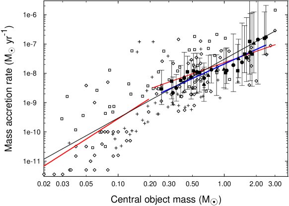
Figure 1.— Mass accretion rates versus stellar masses. The open diamonds represent measurements of TTS and BD from Muzerolle et al. (2005, and references therein); the open squares and crosses represent the confirmed detections and upper limits, respectively, compiled by Natta et al. (2006). The filled triangles, filled circles, and filled squares show the time-averaged quantities for the models with $\gamma=\gamma_{1},\gamma_{2},\>{\rm and}\>\gamma_{3}$, respectively. The bars represent mean positive/negative deviations from the time-averaged accretion rates in each model. The blue line ($\propto M_{\ast}^{1.7}$) is the least-squares fit to the model data. The black line ($\propto M_{\ast}^{2.0}$) is the least-squares fit to the observed confirmed detections, both TTS and BD. The left and right red lines are the least-squares fits to objects with masses in the range $(0.02-0.2)~{}M_{\odot}$ and $(0.2-3.0)~{}M_{\odot}$, respectively.

3. Accretion rates

Figure 1 shows confirmed detections for the mass accretion rate $\dot{M}$ and stellar mass $M_{\ast}$ for TTS and BD of age $0.5-3$ Myr from two recent observational compilations. The open diamonds represent measurements, mostly in Taurus, that have been compiled by Muzerolle et al. (2005, and references therein); the open squares represent detections in $\rho$ Oph obtained by Natta et al. (2006) and crosses represent their upper limits to nondetections. We have excluded objects in the compilation of Muzerolle et al. (2005) that were later observed by Natta et al. (2006). The least-squares best fit to the observational data, both TTS and BD (upper limits excluded), has an exponent $2.0\pm 0.1$ and is shown in Figure 1 by a black line. This value is often quoted in the literature (see § 1). However, we believe that taking a best fit over the whole mass range of BD and TTS may be misleading. Indeed, if we consider separately the intermediate and upper-mass TTS ($0.25~{}M_{\odot}<M_{\ast}<3.0~{}M_{\odot}$) and lower-mass TTS plus BD ($0.02~{}M_{\odot}<M_{\ast}<0.25~{}M_{\odot}$), then the least-squares best fits to each data sample are distinct. In particular, for lower-mass TTS and BD we obtain an exponent $2.3\pm 0.6$ (left red line), whereas for the intermediate and upper-mass TTS we find a much smaller exponent $1.3\pm 0.3$ (right red line).

The above data hints that different mechanisms may be responsible for accretion as one moves along the sequence of stellar masses. However, the observational method of determining $\dot{M}$ also typically varies across the mass sequence, with significant but differing uncertainties. For TTS, the primary determinant of $\dot{M}$ at the stellar surface is UV excess and veiling (see, e.g. Muzerolle et al., 2003), while for BD the primary means is the fitting of emission line profiles. Muzerolle et al. (2003) point out that the latter is considered less accurate than UV excess measurements; it suffers from uncertainties regarding optical depth, rotation, and inclination effects (see also discussion in Mohanty et al., 2005). Quantitative estimates of error bars for either technique are not available in the literature. However, the agreement between the two methods is within a factor $\sim 3-5$ (Muzerolle et al., 2003) where comparable, and this is much smaller than the spread of observed $\dot{M}$ for a given central object mass, implying that the spread of values is primarily due to physical effects of disk age and initial conditions. We also note that the data set of Natta et al. (2006) is based entirely on emission line estimates of accretion onto BD and TTS.

Figure 1 also shows the time-averaged mass accretion rates $\langle\dot{M}\rangle$ and time-averaged stellar masses $\langle M_{*}\rangle$ for our models with $\gamma=\gamma_{1},\gamma_{2},\>{\rm and}\>\gamma_{3}$, respectively. The mass accretion rate $\dot{M}(t)=-2\pi rv_{r}\Sigma$, where $v_{r}$ is the inflow velocity of gas through the sink cell and $r=5$ AU. For most models, the time average is taken between 0.5 Myr and 3.0 Myr after the formation of the protostar. However, protostars with masses above $2.0~{}M_{\odot}$ may enter the T Tauri phase (class II) when they are older than 0.5 Myr. To exclude a possible input from class 0/class I sources in such cases, we start the time average only when the envelope mass has dropped below $10\%$ of the initial cloud mass. The best fit to our model data points is

$$\langle\dot{M}\rangle=10^{-7.7}\;\langle M_{*}\rangle^{1.7}.$$ (5)

and is represented in Figure 1 with a blue line. The least-squares method generates an uncertainty $\pm 0.1$ in the above exponent. The somewhat shallower best-fit slope to the observational data ($1.3\pm 0.3$, right red line) is likely because the short-lived FU Ori bursts are not sampled observationally given the small number of objects. On the other hand, our numerical models produce FU-Ori-like mass accretion bursts (see Fig. 3), which effectively increase $\langle\dot{M}\rangle$ and steepen the model best-fit slope.

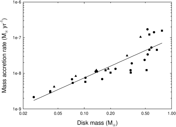
Figure 2.— Time-averaged mass accretion rate $\langle\dot{M}\rangle$ versus time-averaged disk mass $\langle M_{\rm d}\rangle$ for all models. The solid line shows the least-squares fit to the data points. Symbols have the same meaning as in Fig. 1.

It should be noted that our model accretion rates are derived at 5 AU (the sink cell), while the observed accretion rates are measured near the stellar surface. However, our numerical simulations indicate that accretion rates, averaged over many orbital periods, vary little with radius in the inner several tens of AU. Some physical processes operating in the inner several AU and unaccounted in our numerical modeling, will allow accretion onto the stellar surface. The inner accretion rate is expected to match our calculated value when time-averaged, even though it may have significant short term variability.

To quantify the characteristic range of accretion rates obtained in our models, Figure 1 also shows, for each model, the upper and lower bounds on the mass accretion rate $\dot{M}$. These values are obtained by smoothing the accretion rates over $10^{4}$ yr periods (to reduce noise) and typically correspond to the accretion rates at the beginning of the T Tauri phase (upper bound) and at the terminal point of the simulations (lower bound). It is evident that our models can account for the observed range of accretion rates for TTS with masses above $1.0~{}M_{\odot}$. On the other hand, the observed range of accretion rates for the intermediate-mass TTS ($0.25~{}M_{\odot}<M_{\ast}<1.0~{}M_{\odot}$) is greater than that implied by the temporal evolution of our models. We believe that this can be accommodated ultimately by a broader range of initial cloud configurations than we have studied here due to numerical limitations. However, it is remarkable that our models do cover the middle portion of the observed $\dot{M}-M_{\ast}$ phase space.

Figure 2 shows the relation between the time-averaged mass accretion rate $\langle\dot{M}\rangle$ and the time-averaged disk mass $\langle M_{\rm d}\rangle$, to which the least-squares best fit is

$$\langle\dot{M}\rangle=10^{-7.0}\;\langle M_{\rm d}\rangle^{1.1}.$$ (6)

The disk masses are that of matter with surface density above a value 0.1 g cm^-2 that typically characterizes the disk-to-envelope transition (VB07). In our view, equation (6) is the most physically meaningful correlation arising from our simulations of self-consistent disk formation and evolution due to global gravitational torques. However, there is also a mild preference for more massive disks around more massive stars. A plot of $\xi=\langle M_{\rm d}\rangle/\langle M_{*}\rangle$ versus $\langle M_{*}\rangle$ has a best-fit $\xi\propto\langle M_{*}\rangle^{0.3\pm 0.1}$, with values ranging from $\sim 5$% at the low mass end to $\sim 35$% at the high mass end. This serves to steepen the correlation in Figure 1 so that the best fit is $\langle\dot{M}\rangle\propto\langle M_{*}\rangle^{1.7}$.

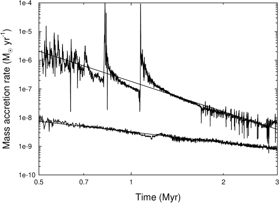
Figure 3.— Mass accretion rate $\dot{M}$ versus time for two models, both with $\gamma=\gamma_{2}$ and initial cloud masses $2.75~{}M_{\odot}$ (top) and $0.35~{}M_{\odot}$ (bottom). The solid lines show the least-squares best fits to the data points.

Finally, Figure 3 shows the typical mass accretion rates obtained in our models as a function of time. The top and bottom lines correspond to models with initial cloud masses $2.75~{}M_{\odot}$ and $0.35~{}M_{\odot}$, respectively, both with $\gamma=\gamma_{2}$. The corresponding time-average protostellar masses are $0.63~{}M_{\odot}$ and $0.026~{}M_{\odot}$, respectively. The more massive disks clearly drive greater mass accretion rates. Furthermore, more massive disks show a wider range of mass accretion rates in the T Tauri phase. The least-squares best fit to the data in Figure 3 yields an exponent $-3.5$ for the $\langle M_{\rm d}\rangle=0.63~{}M_{\odot}$ disk and $-1.2$ for the $\langle M_{\rm d}\rangle=0.026~{}M_{\odot}$ disk. Massive disks have gravitational torques of greater magnitude, which result in greater associated accretion rates. The more massive disk is also violently gravitationally unstable in its early evolution and is characterized by FU-Ori-like accretion bursts (VB05; VB06). We believe that the steeper decline of accretion rate of the $\langle M_{\rm d}\rangle=0.63~{}M_{\odot}$ disk is caused by the greater effect of disk self-gravity and possibly the influence of the more massive stellar object at the center.

4. Conclusions

In this Letter, we have presented models of the late evolution of self-consistently formed protostellar disks that can explain the observed correlation of disk accretion rates with stellar mass for TTS. The formation of the disk and its interaction with the surrounding envelope lead to the development of strong spiral structure during the early evolution of the disk (VB05; VB06). Even after the former has largely disappeared, low-amplitude nonaxisymmetric density perturbations are sustained in the disk for several Myr. The gravitational torques due to these perturbations are sufficient to drive accretion at the rates commonly inferred around TTS. We find that an important property of gravitational torques is that $\langle\dot{M}\rangle$ has an essentially linear dependence on $\langle M_{\rm d}\rangle$. The average disk-to-star mass ratio $\xi$ is in the range $\sim 5\%-35\%$ for models of various masses, given our adopted range of values of initial cloud angular momentum. However, there is a mild trend toward greater values of $\xi$ for models with greater masses. The net result is a best-fit correlation $\langle\dot{M}\rangle\propto\langle M_{*}\rangle^{1.7}$, in good agreement with the observed $\dot{M}-M_{\ast}$ relation.

Since the of values of $\xi$ in our models are $\sim 10$ times greater than estimates made from dust emission (e.g., Andrews & Williams, 2005; Scholz et al., 2006), we anticipate two reasons that this discrepancy may be reduced in the future. Observationally, the inferred gas disk masses may be systematically underestimated using current techniques (see discussion in Hartmann et al., 2006). Theoretically, we need to include additional angular momentum transport mechanisms such as magnetic braking and the magnetorotational instability. We note that only a modest increase in the overall average accretion rate in our current models is required to lead to a dramatic decrease in $\xi$. This is because a small relative increase in the stellar mass can significantly reduce the much smaller disk mass.

References

- Alexander & Armitage (2006) Alexander R. D., & Armitage, P. J. 2006, ApJ, 639, L83
- Andrews & Williams (2005) Andrews, S. M., & Williams, J. P. 2005, ApJ, 631, 1134
- Basu (1997) Basu, S. 1997, ApJ, 485, 240
- Beckwith et al. (1990) Beckwith, S. V. W., Sargent, A. I., Chini, R. S., & Gusten, R. 1990, AJ, 99, 924
- Caselli et al. (2002) Caselli, P., Benson, P. J., Myers, P. C., & Tafalla, M. 2002, ApJ, 572, 238
- Chiang & Goldreich (1997) Chiang, E. I., & Goldreich, P. 1997, ApJ, 490, 368
- Dullemond et al. (2006) Dullemond, C. P., Natta, A., & Testi, L. 2006, ApJ, 645, L69
- Goodman et al. (1993) Goodman, A. A., Benson, P. J., Fuller, G. A., & Myers, P. C. 1993, ApJ, 406, 528
- Hartmann et al. (2006) Hartmann, L., D’Alessio, P., Calvet, N., & Muzerolle, J. 2006, ApJ, 648, 484
- Hartmann et al. (1998) Hartmann, L., Calvet, N., Gullbring, E., & D’Alessio, P. 1998, ApJ, 495, 385
- Klein et al. (2003) Klein, R., Apai, D., Pascucci, I., Henning, Th., & Waters, L. B. F. M. 2003, ApJ, 593, L57
- Mohanty et al. (2005) Mohanty, S., Jayawardhana, R., & Basri, G. 2005, ApJ, 626, 498
- Muzerolle et al. (2003) Muzerolle, J., Hillenbrand, L., Calvet, N., Briceño, C., & Hartmann, L. 2003, ApJ, 592, 266
- Muzerolle et al. (2005) Muzerolle, J., Luhman, K., Briceño, C., Hartmann, L., & Calvet, N. 2005, ApJ, 625, 906
- Narita et al. (1984) Narita, S., Hayashi, C., & Miyama, S. M. 1984, Prog. Theor. Phys., 72, 1118
- Natta et al. (2006) Natta, A., Testi, L., & Randich, S. 2006, A&A, 452, 245
- Norman et al. (1980) Norman, M. L., Wilson, J. R., & Barton, R. T. 1980, ApJ, 239, 968
- Padoan et al. (2005) Padoan, P., Kritsuk, A., Norman, M. L., & Nordlund, A. 2005, ApJ, 622, L61
- Scholz & Jayawardhana (2006) Scholz, A., & Jayawardhana, R. 2006, ApJ, 638, 1056
- Scholz et al. (2006) Scholz, A., Jayawardhana, R., & Wood, K. 2006, ApJ, 645, 1498
- Vorobyov & Basu (2005) Vorobyov, E. I., & Basu, S. 2005, ApJ, 633, L137 (VB05)
- Vorobyov & Basu (2006) Vorobyov, E. I., & Basu, S. 2006, ApJ, 650, 956 (VB06)
- Vorobyov & Basu (2007) Vorobyov, E. I., & Basu, S. 2007, MNRAS, 381, 1009 (VB07)