Constrained MaxLik reconstruction of multimode photon distributions

Abstract

We address the reconstruction of the full photon distribution of multimode fields generated by seeded parametric down-conversion (PDC). Our scheme is based on on/off avalanche photodetection assisted by maximum-likelihood (MaxLik) estimation and does not involve photon counting. We present a novel constrained MaxLik method that incorporates the request of finite energy to improve the rate of convergence and, in turn, the overall accuracy of the reconstruction.

1 Introduction

The reconstruction of photon statistics of quantum optical fields is of the utmost relevance for several applications, ranging from quantum information [1] to the foundations of quantum mechanics [2] and quantum optics [3, 4, 5, 6, 7]. Despite this fact, the realization of photodetectors well suited for this purpose still represents an experimental challenge. The few existing examples [8, 9, 10, 11, 12, 13] show severe limitations. On the other hand, reconstruction schemes based on quantum tomography [14, 15, 16] require phase-matching with a suitable local oscillator and do not represent a technique suited for a diffuse use. This situation prompted various theoretical studies [17, 18, 19, 20] addressed to achieve the reconstruction of the (diagonal) elements of the density matrix exploiting the information achievable with realistic detectors.

In a recent series of papers [21, 22, 23, 24, 25], we have demonstrated how a very satisfactory reconstruction of the statistics of mono-partite and bi-partite quantum optical states may be obtained using the simplest kind of detectors, namely on/off detectors [19, 20] operating in the Geiger mode, whose outcomes are either “off” (no photons detected) or “on”, i.e., a “click”, indicating the detection of one or more photons. Our method recovers the full photon statistics using maximum likelihood (MaxLik) reconstruction on on/off data obtained using variable detection efficiency (by inserting calibrated neutral filters).

In this paper we present a modified version of our method, which improves both convergence and accuracy upon incorporating the obvious a priori constraint of finite signal energy. In particular, we address the reconstruction of the full photon distribution of multimode fields generated by seeded parametric down-conversion. The novel method allows to overcome the increased complexity of the reconstruction problem and represents an important step in view of a widespread application of MaxLik reconstruction.

The paper is structured as follows: in the next Section we describe the constrained MaxLik algorithm in some details, whereas in Section 3 we describe the experimental apparatus and illustrate the application of the method to the reconstruction of the photon distribution of multimode fields generated by seeded parametric down-conversion. Finally, Section 4 closes the paper with some concluding remarks.

2 Constrained MaxLik algorithm

The probability $p_{0}(\eta)$ that a photodetector with quantum efficiency $\eta$ does not click, when an input quantum state $\varrho=\sum_{n,m}\varrho_{nm}|n\rangle\langle m|$ impinges on it, reads as follows:

$$p_{0}(\eta)=\sum_{n}(1-\eta)^{n}\varrho_{n},$$ (1)

where $\varrho_{n}=\varrho_{nn}$ is the $n$-th entry of the photon distribution of the input state. Now, if we consider a set of $N$ detectors with different quantum efficiencies $\eta_{\nu}$, $\nu=1,\ldots,N$, then we can write the “off” probabilities as:

$${\sf P}_{\nu}\equiv p_{0}(\eta_{\nu})=\sum_{n}A_{\nu n}\varrho_{n},$$ (2)

where $A_{\nu n}=(1-\eta_{\nu})^{n}$. Looking at Eq. (2) as a statistical model for the parameters $\varrho_{n}$, we can solve it by the MaxLik estimation. We proceed as follows: first of all, we assume there exists a value $\tilde{n}$ such that $\varrho_{n}$ is negligible for $n>\tilde{n}$; we assign the loglikelihood function (with normalized ${\sf P}_{\nu}$), that is the global probability of the sample:

$${\sf L}=\frac{1}{N_{x}}\log\prod_{\nu}\left(\frac{{\sf P}_{\nu}}{\sum_{\lambda}{\sf P}_{\lambda}}\right)^{{\cal N}_{\nu}}=\sum_{\nu}f_{\nu}\log\frac{{\sf P}_{\nu}}{\sum_{\lambda}{\sf P}_{\lambda}},$$ (3)

where $f_{\nu}={\cal N}_{\nu}/N_{x}$ is the experimental frequency of “off” events, ${\cal N}_{\nu}$ being the number of “off” events for a fixed quantum efficiency $\eta_{\nu}$ and $N_{x}$ the total events amount. The MaxLik estimated $\varrho_{n}$ values are the ones maximizing ${\sf L}$. Since the model is linear and the unknowns $\varrho_{n}$ are positive, we can find the expectation-maximization solution of the MaxLik problem by means of an iterative procedure as described in [26, 17, 21, 27, 28], i.e.:

$$\varrho_{n}^{(h+1)}=\frac{\varrho_{n}^{(h)}}{\sum_{m}{\varrho_{m}^{(h)}}}\sum_{\nu}\frac{A_{\nu n}}{(\sum_{\lambda}A_{\lambda n})}\frac{f_{\nu}}{{\sf P}_{\nu}^{(h)}},$$ (4)

where $\varrho_{n}^{(h)}$ is the value of $\varrho_{n}$ evaluated at the $h$-th iteration, and ${\sf P}_{\nu}^{(h)}=\sum_{n}A_{\nu n}\,\varrho_{n}^{(h)}$. The algorithm (4), known to converge unbiasedly to the MaxLik solution, provides a solution once the initial distribution $\varrho_{n}^{(0)}$ is chosen. On the other hand, the initial distribution slightly affects only the convergence rate and not the precision at convergence [19].

As a matter of fact, the solution obtained above corresponds to the best photon distribution fitting the experimental data, i.e., the measured “off” probabilities. However, it is possible that different photon distributions fit the same experimental data, giving rise to a family of suitable distributions. In these cases it could happen that the MaxLik solution, even if in good agreement with the available experimental knowledge, may be different from the actual (unknown) one. Indeed, this is the case of multimode fields when the number of modes grows. In order to overcome this limitation, we developed a modified version of the MaxLik algorithm, which incorporated the constraint of finite energy for the incoming signal, i.e., the quantity $\sum_{n}n\varrho_{n}$. In practice, we maximize the loglikelihood (3) with a constraint on the energy. Now the function to be maximized with respect to $\varrho_{n}$ is:

$${\sf L}_{\beta}={\sf L}-\beta\sum_{n}n\varrho_{n},$$ (5)

${\sf L}$ being given in (3) and $\beta$ being a Lagrange multiplier. The equations $\frac{\partial{\sf L}_{\beta}}{\partial\varrho_{n}}=0$ lead to:

$$\left(\frac{\sum_{\gamma}{\sf P}_{\gamma}}{\sum_{\mu}f_{\mu}}\right)\sum_{\nu}\frac{A_{\nu n}}{\left[\sum_{\lambda}A_{\lambda n}+\beta\,n\left(\frac{\sum_{\gamma^{\prime}}{\sf P}_{\gamma^{\prime}}}{\sum_{\mu^{\prime}}f_{\mu^{\prime}}}\right)\right]}\frac{f_{\nu}}{{\sf P}_{\nu}}=1,$$ (6)

and, then, by multiplying both the sides of Eq. (6) by $\varrho_{n}$, we get a map ${\boldsymbol{T}}\varrho_{n}=\varrho_{n}$, whose fixed point can be obtained by the following iterative solution:

$$\varrho_{n}^{(h+1)}=\frac{\varrho_{n}^{(h)}}{\sum_{m}{\varrho_{m}^{(h)}}}\sum_{\nu}\frac{A_{\nu n}}{\left[\sum_{\lambda}A_{\lambda n}+\beta\,n\left(\frac{\sum_{\gamma^{\prime}}{\sf P}^{(h)}_{\gamma^{\prime}}}{\sum_{\mu^{\prime}}f_{\mu^{\prime}}}\right)\right]}\frac{f_{\nu}}{{\sf P}^{(h)}_{\nu}}.$$ (7)

The parameter $\beta$ can be tuned in order to control the energy of the reconstructed state and improve both the convergence rate and the overall accuracy. Of course, if we take $\beta=0$, then Eq.s (7) and (4) become the same.

Indeed, in order to use Eq. (7) we need to know the input state energy which, in general, cannot be directly accessible from experimental data. However, in cases when a model of the photon distribution of the input state is available, we can estimate indirectly this energy by a simple fit of the “off” probabilities.

In the following, we consider the multimode field obtained by seeded Parametric Down Conversion (PDC). In this case, the photon distribution is expected to have the form:

$$\varrho_{n}=\frac{({N}_{\rm th})^{n}}{(1+{N}_{\rm th})^{n+M}}\,\exp\left(-\frac{|\alpha|^{2}}{1+{N}_{\rm th}}\right)\,L_{n}^{M-1}\left(-\frac{|\alpha|^{2}}{{N}_{\rm th}(1+{N}_{\rm th})}\right),$$ (8)

where $\varrho_{n}\equiv\varrho_{n}({N}_{\rm th},\alpha,M)$ and $L_{n}^{a}(z)$ are the generalized Laguerre polynomials. Eq. (8) represents the convolution of $M$ thermal states ($M$ spatial modes), all with the same average number of thermal photons ${N}_{\rm th}>0$ except for one, displaced by an amount $\alpha$. This model will be justified by the experimental setup described in Section 3. From Eq.s (1) and (8) we can calculate the “off” probability $p_{0}\equiv p_{0}({N}_{\rm th},\alpha,M,\eta)$, that is:

$$p_{0}=\sum_{n=0}^{\infty}(1-\eta)^{n}\,\varrho_{n}({N}_{\rm th},\alpha,M)=\frac{1}{(1+\eta{N}_{\rm th})^{M}}\,\exp\left(-\frac{\eta|\alpha|^{2}}{1+\eta{N}_{\rm th}}\right),$$ (9)

$\eta$ being the quantum efficiency of the on/off photodetector. Notice that, from Eq. (9), one can obtain the relevant cases for a Poissonian input photon distribution (${N}_{\rm th}\to 0$) and for a multithermal one ($\alpha\to 0$). Thanks to Eq. (9), one can evaluate the input state energy ${N}_{\rm th}+|\alpha|^{2}$, and choose a suitable value for $\beta$.

Before the end of this section, it is worth pointing out that if each spatial mode consists of $M^{\prime}$ temporal modes, then the input photon distribution and the “off” probability are still given by Eq.s (8) and (9), respectively, but with ${\cal M}\rightarrow M\times M^{\prime}$ in place of $M$.

3 Experimental test

In order to test the reliability of the algorithm reported in Eq. (7), we applied it to the reconstruction of a stimulated type-I PDC branch, at different stimulation regimes. In our experiment, whose setup is shown in Fig. 1, a CW Argon laser ($\lambda_{\rm pump}=351.1$ nm) pumps a $5\times 5\times 5$ mm type-I BBO crystal, generating PDC. Together with the pump beam, a CW Nd:Yag laser ($\lambda_{\rm seed}=1064$ nm) is injected into the crystal in the proper way to generate stimulated PDC, and we look at the emission in the ${\mathbf{k}}_{\rm stimul}$ direction ($\lambda_{\rm stimul}=524$ nm).

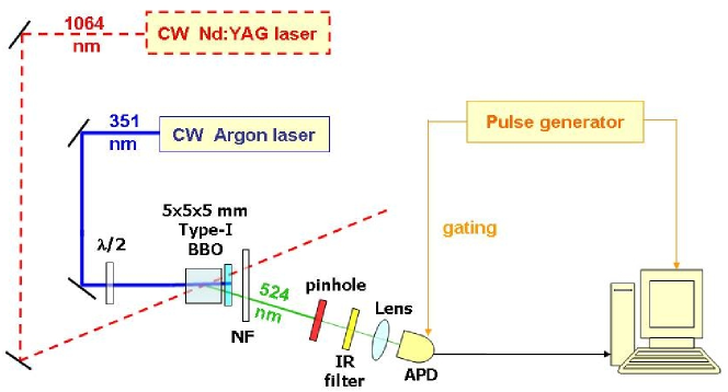
Figure 1: Experimental setup: the stimulated emission at $\lambda_{\rm stimul}=524$ nm is addressed to the NF and then collected by the APD. The number and temporal width of the acquisition windows is set by the pulse generator used for the detector’s gating.

Different values of quantum efficiency have been obtained by inserting properly calibrated Schott neutral filters (NF), starting from $\eta_{\rm max}=28.4\%$; after them, on the optical path of the stimulated branch we put an anti-infrared (IR) filter (to cut off the noise due to the Nd:Yag laser dispersion), a variable pinhole (to control the number $M$ of spatial propagation modes collected) and a fiber coupler connected by a multimode fiber with the detector (avalanche photodiode, Perkin Elmer SPCM-AQR-15). We set the pulse generator in order to open in the APD $2\,10^{5}$ detection windows per second, each one of 20 ns; the pinhole diameter is regulated in order to collect only few spatial modes (more precisely $M=7$), of whom only one stimulated. Moreover, each spatial mode consists of many temporal modes: the total number of modes can then be estimated ${\cal M}=7\,10^{5}$. It is worth to mention that, when the number of modes exceeds few tens, the dependence on this parameter is rather small and a rough estimate of the order of magnitude suffices.

We have performed three separate data collections, each one corresponding to a different stimulation regime: by indicating with $x$ the percentage of stimulated emission on the whole PDC amount collected, our acquisitions were respectively characterized by $x=51.4\%$, $x=78.1\%$ and $x=90.7\%$. The evaluation of the background photons have been performed through an acquisition step without PDC emission (Argon pump off, Nd:Yag seed on), followed by a proper subtraction from data.

\psfrag{P0}{\small$f_{0}$}\psfrag{eta}{\small$\eta$}\psfrag{pn}{\small$\varrho_{n}$}\psfrag{n}{\small$n$}\psfrag{Nave51}{\tiny$N_{\rm ave}=7.23$}\psfrag{x51}{\tiny$x=50.7\%$}\psfrag{chi51}{\tiny$\chi^{2}=4.1\,10^{-2}$}\psfrag{Fid51}{\tiny$F=99.57\%$}\psfrag{Nave78}{\tiny$N_{\rm ave}=16.72$}\psfrag{x78}{\tiny$x=78.1\%$}\psfrag{chi78}{\tiny$\chi^{2}=3.4\,10^{-2}$}\psfrag{Fid78}{\tiny$F=99.97\%$}\psfrag{Nave91}{\tiny$N_{\rm ave}=18.34$}\psfrag{x91}{\tiny$x=90.7\%$}\psfrag{chi91}{\tiny$\chi^{2}=9.1\,10^{-3}$}\psfrag{Fid91}{\tiny$F=99.98\%$}\includegraphics[width=195.12767pt]{51_P0.eps}

\psfrag{P0}{\small$f_{0}$}\psfrag{eta}{\small$\eta$}\psfrag{pn}{\small$\varrho_{n}$}\psfrag{n}{\small$n$}\psfrag{Nave51}{\tiny$N_{\rm ave}=7.23$}\psfrag{x51}{\tiny$x=50.7\%$}\psfrag{chi51}{\tiny$\chi^{2}=4.1\,10^{-2}$}\psfrag{Fid51}{\tiny$F=99.57\%$}\psfrag{Nave78}{\tiny$N_{\rm ave}=16.72$}\psfrag{x78}{\tiny$x=78.1\%$}\psfrag{chi78}{\tiny$\chi^{2}=3.4\,10^{-2}$}\psfrag{Fid78}{\tiny$F=99.97\%$}\psfrag{Nave91}{\tiny$N_{\rm ave}=18.34$}\psfrag{x91}{\tiny$x=90.7\%$}\psfrag{chi91}{\tiny$\chi^{2}=9.1\,10^{-3}$}\psfrag{Fid91}{\tiny$F=99.98\%$}\includegraphics[width=195.12767pt]{51_Pn.eps}

\psfrag{P0}{\small$f_{0}$}\psfrag{eta}{\small$\eta$}\psfrag{pn}{\small$\varrho_{n}$}\psfrag{n}{\small$n$}\psfrag{Nave51}{\tiny$N_{\rm ave}=7.23$}\psfrag{x51}{\tiny$x=50.7\%$}\psfrag{chi51}{\tiny$\chi^{2}=4.1\,10^{-2}$}\psfrag{Fid51}{\tiny$F=99.57\%$}\psfrag{Nave78}{\tiny$N_{\rm ave}=16.72$}\psfrag{x78}{\tiny$x=78.1\%$}\psfrag{chi78}{\tiny$\chi^{2}=3.4\,10^{-2}$}\psfrag{Fid78}{\tiny$F=99.97\%$}\psfrag{Nave91}{\tiny$N_{\rm ave}=18.34$}\psfrag{x91}{\tiny$x=90.7\%$}\psfrag{chi91}{\tiny$\chi^{2}=9.1\,10^{-3}$}\psfrag{Fid91}{\tiny$F=99.98\%$}\includegraphics[width=195.12767pt]{78_P0.eps}

\psfrag{P0}{\small$f_{0}$}\psfrag{eta}{\small$\eta$}\psfrag{pn}{\small$\varrho_{n}$}\psfrag{n}{\small$n$}\psfrag{Nave51}{\tiny$N_{\rm ave}=7.23$}\psfrag{x51}{\tiny$x=50.7\%$}\psfrag{chi51}{\tiny$\chi^{2}=4.1\,10^{-2}$}\psfrag{Fid51}{\tiny$F=99.57\%$}\psfrag{Nave78}{\tiny$N_{\rm ave}=16.72$}\psfrag{x78}{\tiny$x=78.1\%$}\psfrag{chi78}{\tiny$\chi^{2}=3.4\,10^{-2}$}\psfrag{Fid78}{\tiny$F=99.97\%$}\psfrag{Nave91}{\tiny$N_{\rm ave}=18.34$}\psfrag{x91}{\tiny$x=90.7\%$}\psfrag{chi91}{\tiny$\chi^{2}=9.1\,10^{-3}$}\psfrag{Fid91}{\tiny$F=99.98\%$}\includegraphics[width=195.12767pt]{78_Pn.eps}

\psfrag{P0}{\small$f_{0}$}\psfrag{eta}{\small$\eta$}\psfrag{pn}{\small$\varrho_{n}$}\psfrag{n}{\small$n$}\psfrag{Nave51}{\tiny$N_{\rm ave}=7.23$}\psfrag{x51}{\tiny$x=50.7\%$}\psfrag{chi51}{\tiny$\chi^{2}=4.1\,10^{-2}$}\psfrag{Fid51}{\tiny$F=99.57\%$}\psfrag{Nave78}{\tiny$N_{\rm ave}=16.72$}\psfrag{x78}{\tiny$x=78.1\%$}\psfrag{chi78}{\tiny$\chi^{2}=3.4\,10^{-2}$}\psfrag{Fid78}{\tiny$F=99.97\%$}\psfrag{Nave91}{\tiny$N_{\rm ave}=18.34$}\psfrag{x91}{\tiny$x=90.7\%$}\psfrag{chi91}{\tiny$\chi^{2}=9.1\,10^{-3}$}\psfrag{Fid91}{\tiny$F=99.98\%$}\includegraphics[width=195.12767pt]{91_P0.eps}

\psfrag{P0}{\small$f_{0}$}\psfrag{eta}{\small$\eta$}\psfrag{pn}{\small$\varrho_{n}$}\psfrag{n}{\small$n$}\psfrag{Nave51}{\tiny$N_{\rm ave}=7.23$}\psfrag{x51}{\tiny$x=50.7\%$}\psfrag{chi51}{\tiny$\chi^{2}=4.1\,10^{-2}$}\psfrag{Fid51}{\tiny$F=99.57\%$}\psfrag{Nave78}{\tiny$N_{\rm ave}=16.72$}\psfrag{x78}{\tiny$x=78.1\%$}\psfrag{chi78}{\tiny$\chi^{2}=3.4\,10^{-2}$}\psfrag{Fid78}{\tiny$F=99.97\%$}\psfrag{Nave91}{\tiny$N_{\rm ave}=18.34$}\psfrag{x91}{\tiny$x=90.7\%$}\psfrag{chi91}{\tiny$\chi^{2}=9.1\,10^{-3}$}\psfrag{Fid91}{\tiny$F=99.98\%$}\includegraphics[width=195.12767pt]{91_Pn.eps}

Figure 2: On the left: $f_{0}$ non-click frequencies (gray disks) given by the stimulated PDC with different stimulation regimes as functions of the quantum efficiency $\eta$. The black disks are the “off” probabilities obtained by means of the MaxLik reconstructed photon distribution; the solid line corresponds to Eq. (9) with $N_{\rm th}=(1-x)N_{\rm ave}$, $|\alpha|^{2}=xN_{\rm ave}$ and $M=7\,10^{5}$. In each plot we report also the average number of photons ($N_{\rm ave}$) obtained by the fit of the experimental $f_{0}$, the percentage of stimulated emission $x$ and the $\chi^{2}$ of the the MaxLik fit. On the right: MaxLik reconstructed photon distribution (gray bars) and photon distribution given by Eq. (8) with the same values of the parameters given in the respective left plots. In each plot we report also the fidelity $F$ between the two photon distributions. Note the different ranges of $n$.

The obtained results are shown in Figure 2: for the reconstruction we used the MaxLik estimation with constraint on the energy, as described in the previous section. The plots on the left show the $f_{0}$ non-click frequencies given by the stimulated PDC with different stimulation regimes vs. the quantum efficiency $\eta$, and the fit obtained by means of the MaxLik estimation and Eq. (9). The $\chi^{2}$ quantity reported has been defined as the sum of the square differences between the “off” probabilities given by the reconstructed photon statistics and the measured $f_{0}$. To quantify the similarity between the two photon distributions appearing in the plots on the right, instead, we used the fidelity formula:

$$F=\sum_{n}\sqrt{\varrho_{n}^{\rm(ML)}\,\varrho_{n}^{\rm(DMT)}},$$ (10)

where $\varrho_{n}^{\rm(ML)}$ is the MaxLik reconstructed photon distribution and $\varrho_{n}^{\rm(DMT)}$ is the one obtained from Eq. (8).

\psfrag{P0}{\small$f_{0}$}\psfrag{eta}{\small$\eta$}\psfrag{pn}{\small$\varrho_{n}$}\psfrag{n}{\small$n$}\psfrag{NaveNB}{\tiny$N_{\rm ave}=17.55$}\psfrag{xNB}{\tiny$x=90.7\%$}\psfrag{chiNB}{\tiny$\chi^{2}=6.1\,10^{-3}$}\psfrag{FidNB}{\tiny$F=92.81\%$}\includegraphics[width=195.12767pt]{90_NoBETA_P0.eps}

\psfrag{P0}{\small$f_{0}$}\psfrag{eta}{\small$\eta$}\psfrag{pn}{\small$\varrho_{n}$}\psfrag{n}{\small$n$}\psfrag{NaveNB}{\tiny$N_{\rm ave}=17.55$}\psfrag{xNB}{\tiny$x=90.7\%$}\psfrag{chiNB}{\tiny$\chi^{2}=6.1\,10^{-3}$}\psfrag{FidNB}{\tiny$F=92.81\%$}\includegraphics[width=195.12767pt]{90_NoBETA_Pn.eps}

Figure 3: Same plots as the bottom ones in Figure 2, obtained without the energy constraint on the algorithm (notice that here $N_{\rm ave}=17.55$ whereas previously it was $N_{\rm ave}=18.25$): even if the MaxLik fit of the experimental $f_{0}$ set is good, the fidelity between the MaxLik reconstructed photon distribution and the one given by Eq. (8) is quite low.

In Figure 3 we consider the same scenario giving the bottom plots of Figure 2, but now we try to perform the reconstruction without any constraint on the energy ($\beta=0$). We can see that, even if the MaxLik fit of the $f_{0}$ frequencies (left side) is good, the fidelity between the MaxLik reconstructed photon distribution and the one given by Eq. (8) is quite low (right side): a result that confirms the advantage of using the constrained MaxLik method.

4 Concluding remarks

In this paper we have shown how an important improvement on the convergence of the photon statistics reconstruction code, based on MaxLik estimation applied to on/off detection data, can be achieved by increasing the number of Lagrange multipliers when some ”a priori” knowledge of the state is available. In particular we have addressed the reconstruction of the full photon distribution of multimode fields generated by seeded parametric down-conversion, demonstrating the advantages of the constrained MaxLik method. This achievement represents an important step in view of widespread application of this scheme.

References

- [1] Bouwmeester, D.; Ekert, A.K.; Zeilinger, A. The Physics of Quantum Information: Quantum Cryptography, Quantum Teleportation, Quantum Computation, Springer, New York, 2000.
- [2] Genovese, M. Physics Reports, 2005, 413/6.
- [3] Vogel, W.; Welsch, D.G. Quantum Optics - An Introduction, Wiley-vch, Berlin, 2001.
- [4] Schleich, W.P. Quantum Optics in Phase Space, Wiley-Vch, Berlin, 2001.
- [5] Perina, J.; Hradil, Z.; Jurco, B. Quantum Optics and Fundamental Physics, Kluwer, Dordrecht, 1994.
- [6] Leonhardt, U. Measuring the Quantum State of Light , Cambridge Univ. Press, Cambridge, 1997.
- [7] Mandel, L.; Wolf, E. Optical Coherence and Quantum Optics, Cambridge Univ. Press, Cambridge, 1995.
- [8] Zambra, G.; Bondani, M., Rev. Sci. Instrum. 2004, 75, 2762-2765.
- [9] Kim, J.; Takeuchi, S.; Yamamoto, Y. Appl. Phys. Lett. 1999, 74, 902-904.
- [10] Peacock, A.; Verhoeve, P.; Rando, N.; van Dordrecht, A.; Taylor, B.G.; Erd, C.; Perryman, M.A.C.; Venn, R.; Howlett, J.; D. J. Goldie, D.J.; Lumley, J.; Wallis, M. Nature 1996, 381, 135-137.
- [11] Zappa, F.; Lacaita, A.L.; Cova, S.D.; Lovati, P. Opt. Eng., 1996, 35, 938-945.
- [12] Achilles, D.; Silberhorn, C.; Liwa, C.; Banaszek, K.; Walmsley, I.A. Opt. Lett. 2003, 28, 2387-2389.
- [13] Di Giuseppe, G.; Sergienko, A.V.; Saleh, B.E.A.; Teich, M.C. Quantum Information and Computation, Proc. SPIE, 2003 5105, 39-50.
- [14] Munroe, M.; Boggavarapu, D.; Anderson, M.E.; Raymer, M.G. Phys. Rev. A , 1995, 52, 924-927.
- [15] Zhang, Y.;, Kasai, K.; Watanabe, M. Opt. Lett., 2002, 27, 1244-1246.
- [16] Raymer, M.; Beck, M. Quantum States Estimation, Lect. Not. Phys., 649, 235-295, Springer, Berlin-Heidelberg, 2004.
- [17] Mogilevtsev, D. Opt. Comm, 1998, 156, 307-310.
- [18] Mogilevtsev, D. Acta Phys.Slov., 1999, 49, 743-748.
- [19] Rossi, A.R.; Olivares, S.; Paris, M.G.A. Phys. Rev. A, 2004, 70, 055801.
- [20] Rossi, A.R.; Paris, M.G.A. E. Phys. Jour. D, 2005, 32, 223-226.
- [21] Zambra, G.; Andreoni, A.; Bondani, M.; Gramegna, M.; Genovese, M.; Brida, G.; Rossi, A.; Paris, M.G.A. Phys. Rev. Lett., 2005, 95, 063602/1-4.
- [22] Gramegna, M.; Genovese, M.; Brida, G.; Bondani, M.; Zambra, G.; Andreoni, A.; Rossi, A.R.; Paris, M.G.A. Laser Physics, 2006, 16, 385-392;
- [23] Brida, G.; Genovese, M.; Gramegna, M.; Paris, M.G.A.; Predazzi, E.; Cagliero, E. Open Systems Information Dynamics, 2006, 13, 333-341.
- [24] Brida, G.; Genovese, M.; Piacentini, F.; Paris, M.G.A. Optics Letters, 2006, 31, 3508.
- [25] Brida, G.; Genovese, M.; Paris, M.G.A.; Piacentini, F.; Predazzi, E.; Vallauri, E. Optics and Spectroscopy, 2007, 103, 95.
- [26] Banaszek, K. Phys. Rev. A, 1998 57, 5013.
- [27] Hradil, Z.; et al., Phys. Rev. Lett., 2006, 96, 230401.
- [28] Olivares, S.; et al., EPL, 2007, 80, 64002.