Large Qudit Limit of One-dimensional Quantum Walks

Abstract

We study a series of one-dimensional discrete-time quantum-walk models labeled by half integers $j=1/2,1,3/2,\cdots$, introduced by Miyazaki et al., each of which the walker’s wave function has $2j+1$ components and hopping range at each time step is $2j$. In long-time limit the density functions of pseudovelocity-distributions are generally given by superposition of appropriately scaled Konno’s density function. Since Konno’s density function has a finite open support and it diverges at the boundaries of support, limit distribution of pseudovelocities in the $(2j+1)$-component model can have $2j+1$ pikes, when $2j+1$ is even. When $j$ becomes very large, however, we found that these pikes vanish and a universal and monotone convex structure appears around the origin in limit distributions. We discuss a possible route from quantum walks to classical diffusion associated with the $j\to\infty$ limit.

I introduction

In contrast with diffusive behavior of classical random walks, in which the standard deviation of walker’s positions from the starting point is proportional to the square root of time-step in the long-time limit, quantum walkers have velocities ADZ93 ; Mey96 ; NV00 ; ABNVW01 ; TM02 ; Kem03 ; Amb03 ; BCA03 ; Ken06 , and probability distributions of pseudovelocity, the position divided by time, are discussed Kon02 ; Kon05 ; GJS04 ; KFK05 ; MKK07 ; Kon07 .

In the present paper we consider a series of discrete-time quantum-walk models on the one-dimensional lattice (i.e. integers) ${\bf Z}=\{\cdots,-2,-1,0,1,2,\cdots\}$, introduced by MKK07 , where models are labeled by half integers $j=1/2,1,3/2,\cdots$. In the model indexed by $j$, the state of quantum walker is described by a $(2j+1)$-component wave function

$$\Psi^{(j)}(x,t)=\left(\begin{array}[]{c}\psi_{j}^{(j)}(x,t)\cr\psi_{j-1}^{(j)}(x,t)\cr\cdots\cr\psi_{-j+1}^{(j)}(x,t)\cr\psi_{-j}^{(j)}(x,t)\end{array}\right),\quad x\in{\bf Z},\quad t=0,1,2,\dots,$$

normalized as $\sum_{x\in{\bf Z}}|\Psi^{(j)}(x,t)|^{2}=1$, where $|\Psi^{(j)}(x,t)|^{2}=[\Psi^{(j)}(x,t)]^{{\dagger}}\Psi^{(j)}(x,t)=\sum_{m=-j}^{j}|\psi^{(j)}_{m}(x,t)|^{2}$. Let $R^{(j)}$ be a quantum coin represented by a $(2j+1)\times(2j+1)$ unitary matrix, whose $(m,m^{\prime})$-component is denoted by $R^{(j)}_{mm^{\prime}}$. In the present paper, when we write matrices and vectors whose elements are labeled by $m,m^{\prime}$, we will assume that the indices $m$ and $m^{\prime}$ run from $j$ to $-j$ in step of $-1$. At each time step, $2j+1$ components of wave function is mixed by the quantum-coin matrix $R^{(j)}$, and then the quantum walker hops to $2j+1$ sites,

$$\psi^{(j)}_{m}(x,t+1) = \sum_{m^{\prime}=-j}^{j}R^{(j)}_{mm^{\prime}}\psi^{(j)}_{m^{\prime}}(x+2m,t),\quad t=0,1,2\cdots.$$ (1)

We use Wigner’s rotation matrices Wig59 ; Mes62 specified by three real parameters called the Euler angles $\alpha,\beta$, and $\gamma$ as the quantum-coin matrix,

$$R^{(j)}_{mm^{\prime}}(\alpha,\beta,\gamma)=e^{-i\alpha m}r^{(j)}_{mm^{\prime}}(\beta)e^{-i\gamma m^{\prime}},\quad-j\leq m,m^{\prime}\leq j$$

with

$$r^{(j)}_{mm^{\prime}}(\beta)=\sum_{\ell}\Gamma(j,m,m^{\prime},\ell)\left(\cos\frac{\beta}{2}\right)^{2j+m-m^{\prime}-2\ell}\left(\sin\frac{\beta}{2}\right)^{2\ell+m^{\prime}-m}.$$

Here

$$\Gamma(j,m,m^{\prime},\ell)=(-1)^{\ell}\frac{\sqrt{(j+m)!(j-m)!(j+m^{\prime})!(j-m^{\prime})!}}{(j-m^{\prime}-\ell)!(j+m-\ell)!\ell!(\ell+m^{\prime}-m)!},$$

and the summation $\sum_{\ell}$ extends over all integers $\ell$, for which the arguments of the factorials are positive or null ($0!\equiv 1$). The position of the quantum walker at time $t$ is denoted by $X^{(j)}_{t}$ and the probability to find a walker at site $x$ at time $t$ is given by

$$P^{(j)}(x,t)\equiv{\rm Prob}(X_{t}^{(j)}=x)=|\Psi^{(j)}(x,t)|^{2}.$$

The ratio $X^{(j)}_{t}/t$ is called the pseudovelocity of walker KFK05 and its $r$-th moment is given as

$$\left\langle\left(\frac{X^{(j)}_{t}}{t}\right)^{r}\right\rangle=\sum_{x\in{\bf Z}}\left(\frac{x}{t}\right)^{r}P^{(j)}(x,t)$$

at each time $t=0,1,2,\cdots$.

For simplicity, we will assume that at the initial time $t=0$ one quantum walker exists at the origin,

$$\Psi^{(j)}(x,0)=\phi_{0}^{(j)}\delta_{x,0}$$

with

$$\phi_{0}^{(j)}={}^{T}(q_{j},q_{j-1},\cdots,q_{-j+1},q_{-j}),$$ (2)

where $q_{m}\in{\bf C}\equiv$ the set of all complex numbers, $-j\leq m\leq j$, with $\sum_{m=-j}^{j}|q_{m}|^{2}=1$. In this paper the left-superscript $T$ denotes the transpose of vector or matrix. We usually call $\phi_{0}^{(j)}$ a $(2j+1)$-component qudit, which the quantum walker possesses at $t=0$,

For $|a|\leq 1$, let

$$\mu(x;a)=\frac{\sqrt{1-a^{2}}}{\pi(1-x^{2})\sqrt{a^{2}-x^{2}}}{\bf 1}_{\{|x|<|a|\}},$$ (3)

where ${\bf 1}_{\{\omega\}}$ is the indicator function of a condition $\omega$; ${\bf 1}_{\{\omega\}}=1$ if the condition $\omega$ is satisfied, ${\bf 1}_{\{\omega\}}=0$ otherwise. We call it Konno’s density function, since it was first introduced by Konno to describe the limit distributions of the standard two-component quantum walks in his weak limit-theorem Kon02 ; Kon05 . In an earlier paper MKK07 , the following limit theorem was proved,

$$\lim_{t\to\infty}\left\langle\left(\frac{X^{(j)}_{t}}{t}\right)^{r}\right\rangle=\int_{-\infty}^{\infty}dv\,v^{r}\nu^{(j)}(v),\quad r=0,1,2,\cdots$$

with

$$\nu^{(j)}(v)=\sum_{m:0<m\leq j}\frac{1}{2m}\mu\left(\frac{v}{2m};\cos\frac{\beta}{2}\right){\cal M}^{(j,m)}\left(\frac{v}{2m}\right)+{\bf 1}_{\{(2j+1)\,\mbox{is odd}\}}\Delta^{(j)}\delta(v),$$ (4)

where ${\cal M}^{(j,m)}(x)$ are polynomials of $x$ of order $2j$. That is, the long-time limit distribution of pseudovelocity of quantum walker is described by superposition of appropriately scaled Konno’s density functions (3) with weight functions ${\cal M}^{(j,m)}(v/2m)$, and a point mass at the origin with intensity $\Delta^{(j)}$, if the number of states $(2j+1)$ is odd. In the previous paper MKK07 , however, explicit expressions for the weight functions ${\cal M}^{(j,m)}(x)$ are given only for $j=1/2,1,$ and $3/2$, since the functions seem to become very complicated as the value of $j$ increases.

In the present paper we will calculate ${\cal M}^{(j,m)}(x)$ for large values of $j$ and study the asymptotics of the limit distributions (4) in the $j\rightarrow\infty$ limit. We will report our observation that, when $j$ becomes very large, complicated structures of the limit distributions are smeared out and a universal monotonic convex-structure appears around the origin. This observation leads us to a discussion on a possible route from quantum walks to classical diffusion. Relationship between the quantum-walk behavior and diffusive behavior of classical random-walk is an important topic in the study of quantum walks BCA03b .

This paper is organized as follows. In Sec.II, hermitian matrix-representations of weight functions ${\bf M}^{(j,m)}(x)$ are introduced and formulas are given for the matrix elements, which are useful to calculate the limit density-functions for large values of $j$. We analyze limit density-functions for large $j$ in Sec.III and clarify the properties of convex structure, which appears around the origin in limit distributions for sufficiently large values of $j$. Crossover phenomenon from quantum walks to classical diffusion associated with the $j\to\infty$ limit is discussed in Sec.IV. Appendices are used for some details of calculations.

II Weight Functions

II.1 Hermitian-matrix representations

We note that the weight functions ${\cal M}^{(j,m)}(x)$ are represented using $(2j+1)\times(2j+1)$ hermitian matrices ${\bf M}^{(j,m)}(x)$ and $(2j+1)$-component initial-qudit (2) as

$${\cal M}^{(j,m)}(x)=[\phi_{0}^{(j)}]^{{\dagger}}[{\bf M}^{(j,m)}(x)]\phi_{0}^{(j)}.$$

In Appendix A, we give the matrices ${\bf M}^{(j,m)}(x)=({\bf M}^{(j,m)}_{m_{1}m_{2}}(x))$ for $j=1/2,1,3/2$ as examples. In general,

$$\overline{\bf M}^{(j,m)}_{m_{2}m_{1}}={\bf M}^{(j,m)}_{m_{1}m_{2}},\quad-j\leq m_{1},m_{2}\leq j,\quad\mbox{(hermitian condition)}$$ (5)

and

$${\bf M}^{(j,m)}_{-m_{2}-m_{1}}(x) = (-1)^{m_{1}+m_{2}+2m}{\bf M}^{(j,m)}_{m_{1}m_{2}}(-x),\quad-j\leq m_{1},m_{2}\leq j.$$ (6)

We found that, if the indices $m_{1}$ and $m_{2}$ satisfy the condition

$$m_{1}\leq m_{2}\quad\mbox{and}\quad m_{1}\geq-m_{2},$$ (7)

we have the expression

$${\bf M}^{(j,m)}_{m_{1}m_{2}}(x)=\frac{1}{2^{2j-1}}\sum_{\ell_{1}}\sum_{\ell_{2}}\Gamma(j,m_{1},m,\ell_{1})\Gamma(j,m_{2},m,\ell_{2})$$

$$\quad\times\sum_{k_{1}=0}^{A^{(j,m,m_{1})}_{\ell_{1},\ell_{2}}}\sum_{k_{2}=0}^{B^{(m,m_{2})}_{\ell_{1},\ell_{2}}}{A^{(j,m,m_{1})}_{\ell_{1},\ell_{2}}\choose k_{1}}{B^{(m,m_{2})}_{\ell_{1},\ell_{2}}\choose k_{1}}(-1)^{k_{1}}x^{k_{1}+k_{2}}f_{\tau}^{(m_{2}-m_{1})}(x)e^{-i(m_{2}-m_{1})\gamma}.$$ (8)

Here the summations $\sum_{\ell_{1}}$ and $\sum_{\ell_{2}}$ extend over all integers of $\ell_{1}$ and $\ell_{2}$, for which the arguments of the factorials are positive or null,

$$A^{(j,m,m_{1})}_{\ell_{1},\ell_{2}}=2j-(m-m_{1})-(\ell_{1}+\ell_{2}),\quad B^{(m,m_{2})}_{\ell_{1},\ell_{2}}=(m-m_{2})+(\ell_{1}+\ell_{2}),$$

and

$$f_{\tau}^{(a)}(x)=\sum_{k_{0}=0}^{[a/2]}\sum_{k_{1}=0}^{k_{0}}\sum_{k_{2}=0}^{k_{1}}{a\choose 2k_{0}}{k_{0}\choose k_{1}}{k_{1}\choose k_{2}}(-1)^{k_{0}+k_{1}}\tau^{a-2(k_{0}-k_{2})}x^{a-2(k_{0}-k_{1})}$$ (9)

with $\tau=\tan(\beta/2)$, where $[z]$ denotes the integer not greater than $z$. For example, $f_{\tau}^{(1)}(x)=\tau x,f_{\tau}^{(2)}(x)=(2\tau^{2}+1)x^{2}-1,f_{\tau}^{(3)}(x)=(4\tau^{3}+3\tau)x^{3}-3\tau x,f_{\tau}^{(4)}(x)=(8\tau^{4}+8\tau^{2}+1)x^{4}-(8\tau^{2}+2)x^{2}+1$. Note that $f_{\tau}^{(a)}(x)$ is even (respectively, odd) if $a$ is even (respectively, odd). The derivation of (8) is tedious but straightforward following the method given in KFK05 ; MKK07 . The key formulas are found in Appendix C of MKK07 . Combination of the expression (8) with the symmetry properties (5) and (6) determines all elements of the matrix ${\bf M}^{(j,m)}(x)$ for any given $j\in\{1/2,1,3/2,\cdots\}$ and $m\in\{-j,-j+1,\cdots,j\}$.

II.2 Recurrence formulas

As shown in Appendix B, from our expression (8), we can derive the following recurrence formula for matrix elements ${\bf M}^{(j,j)}_{m_{1}m_{2}}(x)$, when the condition (7) is satisfied,

$${\bf M}^{(j,j)}_{m_{1}m_{2}}(x) = \frac{1}{2}c(j;m_{1},m_{2})(1-x){\bf M}^{(j-1/2,j-1/2)}_{m_{1}-1/2\,m_{2}-1/2}(x){\bf 1}_{\{m_{1}\neq-j\}}$$ (10)

$$\quad+\frac{1}{2^{2j-1}}f^{(2j)}_{\tau}(x)e^{-2ij\gamma}{\bf 1}_{\{m_{1}=-j,m_{2}=j\}},$$

where

$$c(j;m_{1},m_{2})=\frac{2j}{\sqrt{(j+m_{1})(j+m_{2})}}.$$

By solving this recurrence formula under the initial condition (16), and by using the symmetry properties (5) and (6), matrices ${\bf M}^{(j,j)}(x)$ can be easily calculated even for large $j$. Moreover, (8) gives the following relation,

$${\bf M}^{(j,j-1)}_{m_{1}m_{2}}(x)=\frac{2(jx+m_{1})(jx+m_{2})}{j(1-x)(1+x)}{\bf M}^{(j,j)}_{m_{1}m_{2}}(x),$$ (11)

which enables us to determine ${\bf M}^{(j,j-1)}(x)$ from ${\bf M}^{(j,j)}(x)$.

III Analysis of Limit Distributions for Large $j$

III.1 Numerical evaluation of exact formula

Though the formula (8) with (9) is rather complicated, it is exact for any given values of $j,m,m_{1}$ and $m_{2}$. Therefore, if we fix the value of $x$, it is easy to evaluate ${\bf M}^{(j,m)}_{m_{1}m_{2}}(x)$ with any precision using computer. In order to demonstrate validity of this procedure, here we compare the numerical evaluations of our exact formula (8) with the results of direct computer-simulations MKK07 of the quantum-walk models for a relatively large value of $j$. As an example, we set $j=11/2$ and $(\alpha,\beta,\gamma)=(0,\pi/2,\pi)$. The initial qudit has $2j+1=12$ complex components. Figure 1(a) shows the result, when we choose the initial qudit as $\phi_{0}={}^{T}((1+i)/2,0,0,0,0,0,0,0,0,0,0,(1-i)/2)$, where the thick lines show the exact limit-distribution of pseudovelocity $\nu^{(11/2)}(v)$ obtained by the above mentioned numerical calculation and the scattering dots indicate the distribution of $X_{t}/t$ at time step $t=100$ obtained by direct computer-simulation. For this initial qudit, the limit probability-density $\nu^{(11/2)}(v)$ is symmetric and well describes the distribution of $X_{t}/t$ for large $t$. If we choose the initial qudit as $\phi={}^{T}(1+i,0,1+i,1,i,i,1+i,i,i,1+i,i,1+i)$ the distribution becomes asymmetric as shown by Fig.1(b).

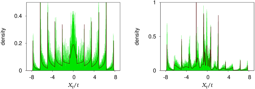
Figure 1: (Color online) Comparison between direct simulation results and the probability densities of limit distributions for the twelve-component model. (a) Symmetric and (b) asymmetric cases.

Figure 1(a) shows that the limit distribution for the $j=11/2$ model (twelve-component model) is given by superposition of six Konno’s density functions (3), each of which is appropriately scaled according to Eq.(4). In addition to them, inside of the innermost Konno’s density function, we can see a convex structure in Fig.1(a)

III.2 The convex structure

From now on we fix the parameters of quantum coins as $\alpha=\gamma=0$ and the form of the initial qudits as $\phi_{0}={}^{T}(q,0,\cdots,0,\bar{q})$ with $q=(1+i)/2$. In order to avoid Dirac’s delta-function peaks, we will assume that the number of states $2j+1$ is even. Now we see the $j$-dependence of central convex structures. Figure 2 shows the central parts of limit distributions with a fixed window, $X_{t}/t\in[-2,2]$, for variety of $j$’s, when we set $\beta=\pi/2$. When $2j+1\geq 8$, we see convex structures for $\beta=\pi/2$.

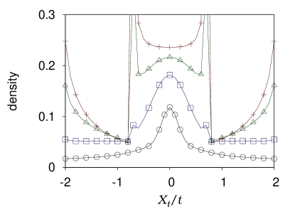
Figure 2: (Color online) Central parts of limit distributions for the models with $2j+1=6$ (plotted by crosses), 8 (triangles), 14 (squares), and 50 (circles). The convex structure appears around the origin, when the number of states with $2j+1$ becomes greater than eight for $\beta=\pi/2$.

In order to verify the fact that, for any value of parameter $\beta$, the convex-structure appears around the origin, if the number of state $2j+1$ becomes sufficiently large, we calculate the second derivative of the density of limit distribution (4). By using the exact expression of weight functions given in Subsection II.A, we have obtained the result,

$$\frac{d^{2}\nu^{(j)}(v)}{dv^{2}}\Bigg{|}_{v=0}=\frac{\sqrt{1-\cos^{2}(\beta/2)}}{\pi\cos(\beta/2)}$$

$$\quad\times\sum_{0<m\leq j}\frac{1}{8m^{3}}\left[\left\{2+\frac{1}{\cos^{2}(\beta/2)}+2(2m^{2}-j)\right\}\frac{(2j)!}{2^{2j-1}(j+m)!(j-m)!}\right].$$ (12)

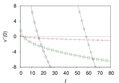
Figure 3: (Color online) Values of second derivatives of limit density-functions at the origin are plotted for various $\beta$. Crosses are for $\beta=\pi/10$, squares for $\beta=\pi/2$, circles for $\beta=22\pi/25$, and triangles for $\beta=46\pi/50$, respectively.

In Fig.3 we plot the values of (12) with changing values of $j$ for $\beta=\pi/10,\pi/2,22\pi/25$ and $47\pi/50$. As demonstrated by this figure, we can prove that for any given $\beta\in[0,\pi]$, these is a critical value $j_{c}(\beta)$ such that $d^{2}\nu^{(j)}(v)/dv^{2}|_{v=0}<0$ for all $j>j_{c}(\beta)$.

III.3 Smoothing by weight function in large $j$

As given by Eq.(4), the probability density of limit distribution of pseudovelocities is given by superposing Konno’s density functions (3) appropriately scaled. Since each Konno’s density function $\mu(v/2m;\cos(\beta/2))$ has a finite open support $v\in(-2m\cos(\beta/2),2m\cos(\beta/2))$ and diverges at the boundaries of it, we see pikes at $v=\pm 2m\cos(\beta/2)$, $0<m\leq j$, in the limit distribution as shown by Fig.1(a), which was given for the case $2j+1=12$ and $\beta=\pi/2$.

For a given value of parameter $\beta$, however, if we set $j\gg j_{c}(\beta)$, limit distributions seem to be quite different from that shown in Fig.1(a). Figure 4(a) shows the limit distribution for the $2j+1=50$ case with $\beta=\pi/2$. Pikes vanish in a central region and the convex structure at the origin becomes very evident.

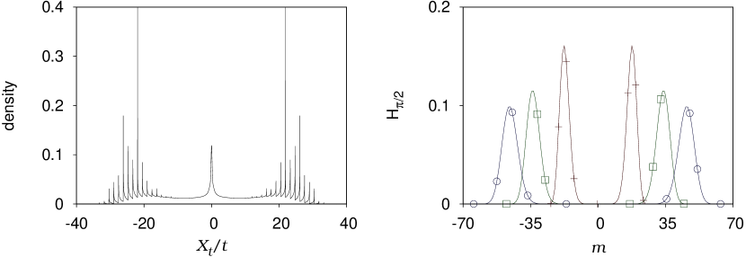
Figure 4: (Color online) (a) Probability density of limit distribution for the case $2j+1=50$, $\beta=\pi/2$. (b) Functions $H_{\pi/2}(m)$ plotted for the cases $2j+1=50$ (crosses), 96 (squares), and 130 (circles).

This smoothing phenomenon is caused by the interesting property of weight functions ${\cal M}^{(j,m)}$; for large $j$, ${\cal M}^{(j,m)}(v/2m)$ becomes to attain zeros at the points $v=\pm 2m\cos(\beta/2),0<m\leq j$, where the scaled Konno’s density functions, $\mu(v/2m;\cos(\beta/2))$, diverge. In order to see this fact, for given $j$ and $\beta$, we define a function of $m$ by

$$H^{(j)}_{\beta}(m) = {\cal M}^{(j,m)}(\cos\beta/2)$$

$$= \frac{(2j)!}{2^{2j-1}}\sum_{k_{1}=0}^{j+m}\sum_{k_{2}=0}^{j-m}\frac{(-1)^{k_{1}}(\cos(\beta/2))^{k_{1}+k_{2}}}{k_{1}!(j+m-k_{1})!k_{2}!(j-m-k_{2})!}{\bf 1}_{\{k_{1}+k_{2}\,\mbox{is even}\}},$$

$0<m\leq j$. Figure 4(b) shows the functions, when $\beta=\pi/2$, for the cases $2j+1=50,96$ and $130$. As increasing $j$, the central region, where $H_{\beta}^{(j)}(m)=0$, becomes wider.

III.4 Rescaling of limit density-function

By definition of our models, the range of elementary hopping of quantum walker at each time step is $2j$; see Eq.(1). Then distribution of pseudovelocities of quantum walker spreads in an interval $(-2j\cos(\beta/2),2j\cos(\beta/2))$.

In order to discuss the $j\to\infty$ limit of the series of our models, here we introduce the rescaled variable

$$\widetilde{X}_{t}^{(j)}=\frac{X_{t}^{(j)}}{2j\cos(\beta/2)}$$ (13)

for each value of $\beta$. Figure 5(a) shows the limit density-functions of the rescaled pseudovelocities $\widetilde{X}^{(j)}_{t}/t$ for $2j+1=10,20$ and $50$. In this variable, the support of the limit distribution is fixed to be $(-1,1)$. As shown by Fig.5(a), the central convex structure becomes sharper monotonically in increasing the value of $j$. Corresponding to (13), we plot $\sigma_{j}H_{\beta/2}$’s as functions of $m/{\sigma_{j}}$, where $\sigma_{j}=\sqrt{2}j$, in Fig.5(b) for $\beta=\pi/2$. It is interesting to see that the locations, where the functions take non-zero values, are now fixed.

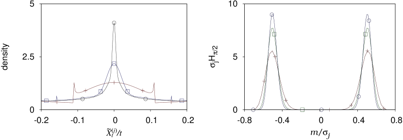
Figure 5: (Color online) (a) Central parts of density functions of limit distributions of rescaled pseudovelocities for $2j+1=10$ (crosses), 20 (squares), and 50 (circles). (b) $\sigma_{j}H_{\beta}(m)$ versus $m/\sigma_{j}$ with $\sigma_{j}=\sqrt{2}j$ for $2j+1=50$ (crosses), 96 (squares) and 130 (circles), when $\beta=\pi/2$.

IV Discussion

Now we discuss the $j\to\infty$ limit of the present series of one-dimensional quantum-walk models. If we consider the situation that $j$ is finite but very large, the limit distribution of the rescaled pseudovelocity $\widetilde{X}^{(j)}_{t}/t$ will have a simple profile. There will be a sharp convex structure at the origin and accumulations of pikes only in the very vicinity of the boundary points -1 and 1 of the support of limit density-function, but in other regions in the support the density of distribution will be almost zero. In the $j\to\infty$ limit, the central convex-structure will become a single point mass (i.e. a Dirac delta-function) at the origin. It implies that the pseudovelocity is almost zero, that is, the quantum walk will lose its velocity in the $j\to\infty$ limit.

In the series of one-dimensional quantum-walk models studied in the present paper, we have used Wigner’s rotation matrices $R^{(j)}$ as quantum coins. We should note that $R^{(j)}$ is introduced Wig59 ; Mes62 , when rotations in the three-dimensional real space are quantized and the index $j$ is defined as a quantum number, which specify physical states allowed in the quantum mechanics.

In the standard quantum mechanics, a small but finite parameter $\hbar$ (the Planck constant divided by $2\pi$) is introduced and physical quantities are quantized to have only discrete values of the form $\hbar\times\mbox{(quantum numbers)}$. For example the energy levels of a harmonic oscillator with the angular frequency $\omega$ are given by $E_{n}=\hbar\omega(n+1/2),n=0,1,2,\dots$, and the square of angular momentum ${\bf L}$ and its $z$-component are given by ${\bf L}^{2}=\hbar^{2}\ell(\ell+1)$ and $L_{z}=\hbar m$, $\ell=0,1/2,1,3/2,\cdots,m=-\ell,-\ell+1,\cdots,\ell$. If the quantum system involves $\hbar$ explicitly, it is easy to consider its classical correspondence by taking the limit $\hbar\to 0$. Even though the system does not include the parameter $\hbar$ explicitly, the classical limit can be realized by taking a large quantum-number limit, since physical quantities should be given of the form $\hbar\times\mbox{(quantum numbers)}$ as the above examples show.

Then we can expect that, if we take $j\to\infty$ limit appropriately, the classical diffusive behavior will be observed BCA03b . One possibility is to see a crossover phenomenon from quantum-walk behavior to classical diffusion in $j\to\infty$. Assume the form $X_{t}^{(j)}\sim jtF(t/j^{\theta})$ with a scaling function $F(z)$ such that $F(z)\sim z^{-1/2}$ in $z\to 0$ and $F(z)\to$ const. in $z\to\infty$, where $\theta$ is an exponent. For finite $j$, $X_{t}^{(j)}\sim jt$ in $t\to\infty$, as we have shown in the present paper. On the other hand, for finite $t$, we will have $X_{t}^{(j)}\sim(jt)(t/j^{\theta})^{-1/2}=j^{1+\theta/2}\sqrt{t}$ in $j\to\infty$; that is, $X^{(j)}_{t}/j^{1+\theta/2}$ is diffusive in large $t$. It will be an interesting future problem to clarify the phenomena, which are realized when we take a proper classical limit in the series of quantum-walk models.

Appendix A The matrices ${\bf M}^{(j,m)}(x)$ for $j=1/2,1,3/2$

Let $\tau=\tan(\beta/2)$ and $f_{\tau}^{(1)}(x)=\tau x,f_{\tau}^{(2)}(x)=(2\tau^{2}+1)x^{2}-1$. Then

$${\bf M}^{(1/2,1/2)}(x)=\left(\begin{array}[]{ll}1-x&\tau xe^{i\gamma}\\ \tau xe^{-i\gamma}&1+x\\ \end{array}\right),$$ (16)

$${\bf M}^{(1,1)}(x)=\left(\begin{array}[]{lll}\frac{1}{2}(1-x)^{2}&\frac{\sqrt{2}}{2}(1-x)f_{\tau}^{(1)}(x)e^{i\gamma}&\frac{1}{2}f_{\tau}^{(2)}(x)e^{2i\gamma}\\ \frac{\sqrt{2}}{2}(1-x)f_{\tau}^{(1)}(x)e^{-i\gamma}&(1-x)(1+x)&\frac{\sqrt{2}}{2}(1+x)f_{\tau}^{(1)}(x)e^{\gamma}\\ \frac{1}{2}f_{\tau}^{(2)}(x)e^{-2i\gamma}&\frac{\sqrt{2}}{2}(1+x)f_{\tau}^{(1)}(x)e^{-i\gamma}&\frac{1}{2}(1+x)^{2}\\ \end{array}\right),$$ (20)

$${\bf M}^{(3/2,3/2)}(x)$$ (25)

$$= \left(\begin{array}[]{llll}\frac{1}{4}(1-x)^{3}&\frac{\sqrt{3}}{4}(1-x)^{2}f_{\tau}^{(1)}(x)e^{i\gamma}&\frac{\sqrt{3}}{4}(1-x)f_{\tau}^{(2)}(x)e^{2i\gamma}&\frac{1}{4}f_{\tau}^{(3)}(x)e^{3i\gamma}\\ \frac{\sqrt{3}}{4}(1-x)^{2}f_{\tau}^{(1)}(x)e^{-i\gamma}&\frac{3}{4}(1-x)^{2}(1+x)&\frac{3}{4}(1-x)(1+x)f_{\tau}^{(1)}(x)e^{i\gamma}&\frac{\sqrt{3}}{4}(1+x)f_{\tau}^{(2)}(x)e^{2i\gamma}\\ \frac{\sqrt{3}}{4}(1-x)f_{\tau}^{(2)}(x)e^{-2i\gamma}&\frac{3}{4}(1-x)(1+x)f_{\tau}^{(1)}(x)e^{-i\gamma}&\frac{3}{4}(1-x)(1+x)^{2}&\frac{\sqrt{3}}{4}(1+x)^{2}f_{\tau}^{(1)}(x)e^{i\gamma}\\ \frac{1}{4}f_{\tau}^{(3)}(x)e^{-3i\gamma}&\frac{\sqrt{3}}{4}(1+x)f_{\tau}^{(2)}(x)e^{-2i\gamma}&\frac{\sqrt{3}}{4}(1+x)^{2}f_{\tau}^{(1)}(x)e^{-i\gamma}&\frac{1}{4}(1+x)^{3}\\ \end{array}\right).$$

Appendix B Derivation of EQ.(10)

When $m_{1}\not=-j$, Eq.(8) gives

$$(1-x){\bf M}^{(j-1/2,j-1/2)}_{m_{1}-1/2\,m_{2}-1/2}(x)=\frac{1}{2^{2j-2}}f_{\tau}^{(m_{2}-m_{1})}(x)e^{-i(m_{2}-m_{1})\gamma}$$

$$\quad\times\Gamma\left(j-\frac{1}{2},m_{1}-\frac{1}{2},j-\frac{1}{2},0\right)\Gamma\left(j-\frac{1}{2},m_{2}-\frac{1}{2},j-\frac{1}{2},0\right)$$

$$\quad\times\sum_{k_{1}=0}^{j+m_{1}-1}\sum_{k_{2}=0}^{j-m_{2}}{j+m_{1}-1\choose k_{1}}{j-m_{2}\choose k_{2}}(-1)^{k_{1}}(x^{k_{1}+k_{2}}-x^{k_{1}+k_{2}+1}).$$

The summations over $k_{1}$ and $k_{2}$ are carried out as

$$\sum_{k_{2}=0}^{j-m_{2}}{j-m_{2}\choose k_{2}}x^{k_{2}}\left\{\sum_{k_{1}=0}^{j+m_{1}-1}{j+m_{1}-1\choose k_{1}}(-1)^{k_{1}}x^{k_{1}}-\sum_{k_{1}=0}^{j+m_{1}-1}{j+m_{1}-1\choose k_{1}}(-1)^{k_{1}}x^{k_{1}+1}\right\}$$

$$\quad=\sum_{k_{2}=0}^{j-m_{2}}{j-m_{2}\choose k_{2}}x^{k_{2}}\left\{1+(-x)^{j+m_{1}}+\sum_{k_{1}=1}^{j+m_{1}-1}{j+m_{1}\choose k_{1}}(-1)^{k_{1}}x^{k_{1}}\right\}$$

$$\quad=\sum_{k_{1}=0}^{j+m_{1}}\sum_{k_{2}=0}^{j-m_{2}}{j+m_{1}\choose k_{1}}{j-m_{2}\choose k_{2}}(-1)^{k_{1}}x^{k_{1}+k_{2}}.$$

We note the equality

$$c(j;m_{1},m_{2})\Gamma\left(j-\frac{1}{2},m_{1}-\frac{1}{2},j-\frac{1}{2},0\right)\Gamma\left(j-\frac{1}{2},m_{2}-\frac{1}{2},j-\frac{1}{2},0\right)$$

$$\quad=\Gamma(j,m_{1},j,0)\Gamma(j,m_{2},j,0).$$

Then Eq.(10) is derived. When $m_{1}=-j$, it is enough to only consider the case $m_{2}=j$ under the condition (7). This case is trivial; ${\bf M}^{(j,m)}_{-jj}(x)=2^{-2j+1}f_{\tau}^{(2j)}(x)e^{-2ij\gamma}$.

References

- (1) Y. Aharonov, L. Davidovich, and N. Zagury, Phys. Rev. A 48, 1687 (1993).
- (2) D. A. Meyer, J. Stat. Phys. 85, 551 (1996).
- (3) A. Nayak and A. Vishwanath, e-print quant-ph/0010117.
- (4) A. Ambainis, E. Bach, A. Nayak, A. Vishwanath, and J. Watrous, in Proceedings of the 33rd Annual ACM Symposium on Theory of Computing (ACM Press, New York, 2001), pp.37-49.
- (5) B. C. Travaglione and G. J. Milburn, Phys. Rev. A 65, 032310 (2002)
- (6) J. Kempe, Contemp. Phys. 44, 307 (2003).
- (7) A. Ambainis, Int. J. Quantum Inf. 1, 507 (2003).
- (8) T. A. Brun, H. A. Carteret, and A. Ambainis, Phys. Rev. A 67, 052317 (2003).
- (9) V. M. Kendon, Int. J. Quantum Inf. 4, 791 (2006).
- (10) N. Konno, Quantum Inf. Process 1, 345 (2002).
- (11) N. Konno, J. Math. Soc. Jpn, 57, 1179 (2005).
- (12) G. Grimmett, S. Janson, and P. F. Scudo, Phys. Rev. E 69, 026119 (2004).
- (13) M. Katori, S. Fujino, and N. Konno, Phys. Rev. A 72, 012316 (2005).
- (14) T. Miyazaki, M. Katori, N. Konno, Phys. Rev. A 76 012332 (2007).
- (15) N. Konno, Quantum Walks, Lecture at the School “Quantum Potential Theory: Structure and Applications to Physics” held at the Alfried Krupp Wissenschaftskolleg, Greifswald, 26 February - 9 March 2007. (Reihe Mathematik, Ernst-Moritz-Arndt-Universität Greifswald, No.2, 2007.) The lecture note is available at http://www.math-inf.uni-greifswald.de/algebra/qpt/konno-26nov2007.
- (16) E. P. Wigner, Group Theory and Its Application to the Quantum Mechanics of Atomic Spectra (Academic Press, New York, 1959).
- (17) A. Messiah, Quantum mechanics, vol. II, (North Holland, Amsterdam, 1962).
- (18) T. A. Brun, H. A. Carteret, and A. Ambainis, Phys. Rev. Lett. A 91, 130602 (2003).