Resonant cyclotron scattering in magnetars’ emission

Abstract

We present a systematic fit of a model of resonant cyclotron scattering (RCS) to the X-ray data of ten magnetars, including canonical and transient anomalous X-ray pulsars (AXPs), and soft gamma repeaters (SGRs). In this scenario, non-thermal magnetar spectra in the soft X-rays (i.e. below $\sim 10$ keV) result from resonant cyclotron scattering of the thermal surface emission by hot magnetospheric plasma. We find that this model can successfully account for the soft X-ray emission of magnetars, while using the same number of free parameters than the commonly used empirical blackbody plus power-law model. However, while the RCS model can alone reproduce the soft X-ray spectra of AXPs, the much harder spectra of SGRs below 10 keV, requires the addition of a power-law component (the latter being the same component responsible for their hard X-ray emission). Although this model in its present form does not explain the hard X-ray emission of a few of these sources, we took this further component into account in our modeling not to overlook their contribution in the $\sim$4-10 keV band. We find that the entire class of sources is characterized by magnetospheric plasma with a density which, at resonant radius, is about 3 orders of magnitudes higher than $n_{GJ}$, the Goldreich-Julian electron density. The inferred values of the intervening hydrogen column densities, are also in better agreement with more recent estimates inferred from the fit of single X-ray edges. For the entire sample of observations, we find indications for a correlation between the scattering depth and the electron thermal velocity, and the field strength. Moreover, in most transient anomalous X-ray pulsars the outburst state is characterized by a relatively high surface temperature which cools down during the decay, while the properties of the magnetospheric electrons vary in a different way from source to source. Although the treatment of the magnetospheric scattering used here is only approximated, its successful application to all magnetars we considered shows that the RCS model is capable to catch the main features of the spectra observed below $\sim 10$ keV.

1 Introduction

The neutron star world, as we knew it until not long ago, appeared mainly populated by radio pulsars (PSRs, about 2000 objects). In the last two decades diverse, puzzling classes of isolated neutron stars (NSs), with properties much at variance with those of canonical PSRs, were discovered: the anomalous X-ray pulsars (AXPs), the soft gamma repeaters (SGRs; Woods & Thompson 2006; Mereghetti 2008), the rotating radio transients (RRATs; McLaughlin et al. 2006), and the X-ray dim isolated neutron stars (XDINSs; Haberl 2007). Among these, the AXPs and SGRs are, in some sense, the most peculiar, since they are believed to host ultra-magnetized NSs, with a magnetic field $\approx 10^{14}$–$10^{15}$ G, in excess of the critical magnetic field, $B_{crit}\equiv m_{e}^{2}c^{3}/(e\hbar)=4.414\times 10^{13}$ G, at which the cyclotron energy equals the rest mass energy for an electron (Duncan & Thompson 1992; Thompson & Duncan 1993, 1995, 1996).

The magnetar candidates (about fifteen known objects) are characterized by slow X-ray pulsations ($P\sim 2$–12 s) and large spin-down rates ($\dot{P}\sim 10^{-10}$–$10^{-12}$ s s^-1). A distinctive property is their high persistent X-ray luminosity ($L\approx 10^{34}$–$10^{36}$erg s^-1), which exceeds the spin-down luminosity typically, by two orders of magnitude. Thus, magnetar X-ray emission can not be explained in terms of rotational energy losses. Measurements of spin periods and period derivatives, assuming that the latter are due to electromagnetic dipolar losses, lend further support to the idea that these objects contain neutron stars endowed with an ultra-strong magnetic field. Although the magnetar model has become increasingly popular, alternative scenarios to explain the enigmatic properties of these sources have been proposed. Among these, models involving accretion from a fossil disk, formed in the supernova event which gave birth to the neutron star, are still largely plausible (e.g. van Paradijs et al. 1995; Chatterjee, Hernquist & Narayan 2000; Perna, Heyl & Hernquist 2000).

Magnetar X-ray emission may be qualitatively separated into two components, a low-energy, $\lesssim 10$  keV, and a high-energy one, $\gtrsim 20$  keV. It is likely, although not proved yet, that different emission mechanisms are responsible for the two components. The low energy component is typically fit with either a blackbody with a temperature $kT\sim 0.3-0.6$  keV and a power-law with a relatively steep photon index, $\Gamma\sim 2$–4, or two blackbodies with $kT_{1}\sim 0.3$ keV and $kT_{2}\sim 0.7$ keV (see Woods & Thompson 2006 and Mereghetti 2008 for a review). In a few cases the low-energy component of SGR spectra has been fit with a single power-law, but recent longer observations have shown that, also for these sources, a blackbody component is required (Mereghetti et al. 2005a). The high-energy component, discovered from four AXPs (Kuiper et al. 2004, 2006) and two SGRs (Mereghetti et al. 2005b; Molkov et al. 2005; Götz et al. 2006) has in general a quite hard spectrum (modeled by a power-law), and accounts for about half of the bolometric luminosity of these sources. This makes it crucial to consider in any spectral modeling the whole 1–200 keV spectrum, where $>90\%$ of the magnetar emission is concentrated, instead of focussing on the soft X-ray range alone. Furthermore, the discovery of magnetar counterparts in the radio and infrared/optical bands (Camilo et al. 2006; Hulleman et al. 2000) enforced the idea that their multi-wavelength spectral energy distribution is by far more complex than the simple superposition of blackbody (BB) and power-law (PL) distributions.

The purpose of this paper is to provide a physical interpretation of the soft X-ray component ($\lesssim 10$ keV) through a detailed analysis of magnetar spectra. Our starting point is the work by Thompson, Lyutikov & Kulkarni (2002, TLK in the following), who pointed out that resonant scattering in magnetar magnetospheres may explain the non-thermal emission observed in magnetar candidates. Due to the presence of hot plasma in the neutron star coronae, the thermal emission from the neutron star surface/atmosphere gets distorted through efficient resonant cyclotron scattering. Resonant cyclotron scattering has been first studied in the accretion columns of neutron star X-ray binary systems or in their atmospheres (Wasserman & Salpenter 1980; Nagel 1981; Lamb, Wang & Wasserman 1990). Lyutikov & Gavriil (2006) computed, in an approximated and semi-analytical way, the effect of multiple resonant scatterings of soft photons in the magnetosphere, and found that the emerging spectrum is non-thermal, with a shape that may resemble the observed blackbody plus power-law. This model was preliminarily fit to the spectrum of the AXP 1E 1048-5937   (Lyutikov & Gavriil 2006), although the magnetospheric parameters were held fixed during the modeling. Rea et al. (2007a,b) implemented in XSPEC a more refined version in which also these parameters are minimized during the fit (see §2.2), and successfully modeled a simultaneous Swift  and INTEGRAL   observation of 4U 0142+614 . In the following, we refer to this XSPEC model as the RCS model, where RCS stands for Resonant Cyclotron Scattering. Güver et al. (2007a,b) fit a similar model to two AXPs, taking into account for the fact that the thermal emission from the star surface is not a blackbody if the presence of an atmosphere is accounted for (see also §5). More detailed, fully 3D Monte Carlo simulations of multiple resonant scattering in the star magnetosphere have been very recently presented by Fernandez & Thompson (2007; see also Nobili, Turolla & Zane 2008) but not directly applied to the data yet (this will be done in a subsequent paper).

In this paper we present a systematic application of the RCS model to observations of all AXPs and SGRs. We consider the deepest X-ray pointings available up to now for these sources, obtained making use of the large throughput of the XMM–Newton   satellite. For a subset of sources, which have been detected in the hard X-ray range, we also consider a joint fit with the INTEGRAL   spectra in order to study systematically the relation between hard and soft X-rays production mechanisms.

The paper is organized as follows. The basic concepts behind the RCS model and its XSPEC implementation are summarized in § 2. In §3 we report the observations and the data analysis. Results of the spectral modeling are presented in §4, and discussed in §5. Conclusions follow.

2 Resonant Cyclotron Scattering

2.1 The model

Before discussing our XSPEC model and the implications of our results, we briefly touch on some properties of the RCS model which directly bear to the physical interpretation of the fitting parameters and their comparison with similar parameters introduced in other theoretical models. The basic idea follows the original suggestion by TLK, who pointed out that a scattering plasma may be supplied to the magnetosphere by plastic deformations of the crust, which twist the external magnetic field and push electric currents into the magnetosphere. The particle density of charge carries required to support these currents may largely exceed the Goldreich-Julian charge density (Goldreich & Julian 1969). Furthermore, it is expected that instabilities heat the plasma.

Following this idea, Lyutikov & Gavriil (2006) studied how magnetospheric plasma might distort the thermal X-ray emission emerging from the star surface through efficient resonant cyclotron scattering. If a large volume of the neutron star magnetosphere is filled by a hot plasma, the thermal (or quasi-thermal) cooling radiation emerging from the star surface will experience repeated scatterings at the cyclotron resonance. The efficiency of the process is quantified by the scattering optical depth, $\tau_{res}$,

$$\tau_{res}=\int\sigma_{res}n_{e}dl=\tau_{0}(1+\cos^{2}\alpha)$$ (1)

where

$$\sigma_{res}={\sigma_{T}\over 4}{(1+\cos^{2}\alpha)\omega^{2}\over(\omega-\omega_{B})^{2}+\Gamma^{2}/4}$$ (2)

is the (non-relativistic) cross-section for electron scattering in the magnetized regime, $n_{e}$ is the electrons number density, $\alpha$ is the angle between the photon propagation direction and the local magnetic field, $\Gamma=4e^{2}\omega_{B}^{2}/3m_{e}c^{3}$ is the natural width of the first cyclotron harmonic, $\sigma_{T}$ is the Thomson scattering cross-section, and

$$\tau_{0}={\pi^{2}e^{2}n_{e}r\over 3m_{e}c\omega_{B}}\,.$$ (3)

Here $r$ is the radial distance from the center of the star, $\omega_{B}=eB/m_{e}c$ is the electron cyclotron frequency, and $B$ is the local value of the magnetic field. At energies corresponding to soft X-ray photons, the resonant scattering optical depth greatly exceeds that for Thomson scattering, $\tau_{T}\sim n_{e}\sigma_{T}r$,

$${\tau_{res}\over\tau_{T}}\sim{\pi\over 8}{m_{e}c^{3}\over e^{2}\omega_{B}}\sim 10^{5}\left(\frac{1\ \mathrm{keV}}{\hbar\omega_{B}}\right)\,.$$ (4)

This implies that even a relatively small amount of plasma present in the magnetosphere of the NS may considerably modify the emergent spectrum.

The RCS model developed by Lyutikov & Gavriil (2006), and used in this investigation, is based on a simplified, 1D semi-analytical treatment of resonant cyclotron up-scattering of soft thermal photons, under the assumption that scattering occurs in a static, non-relativistic, warm medium and neglecting electron recoil. The latter condition requires $\hbar\omega\ll m_{e}c^{2}$. Emission from the neutron star surface is treated assuming a blackbody spectrum, and that seed photons propagate in the radial direction. Magnetospheric charges are taken to have a top-hat velocity distribution centered at zero and extending up to $\pm\beta_{T}$. Such a velocity distribution mimics a scenario in which the electron motion is thermal (in 1D because charges stick to the field lines). In this respect, $\beta_{T}$ is associated to the mean particle energy and hence to the temperature of the 1D electron plasma. Since scatterings with the magnetospheric electrons occur in a thin shell of width $H\sim\beta_{T}r/3\ll r$ around the “scattering sphere”, one can treat the scattering region as a plane-parallel slab. Radiation transport is tackled by assuming that photons can only propagate along the slab normal, i.e. either towards or away from the star. Therefore, $\cos\alpha=\pm 1$ in eq. (1) and it is $\tau_{res}=2\tau_{0}$; the electron density is assumed to be constant through the slab. We notice that the model does not account for the bulk motion of the charges. This is expected since the starting point is not a self-consistent calculation of the currents but a prescription for the charge density. As a consequence, the electron velocity and the optical depth are independent parameters, although in a more detailed treatment this might not be the case (Beloborodov & Thompson 2007).

Although Thomson scattering conserves the photon energy in the electron rest frame, the (thermal) motion of the charges induces a frequency shift in the observer frame. However, since our electron velocity distribution averages to zero, a photon has the same probability to undergo up or down-scattering. Still, a net up-scattering (and in turn the formation of a hard tail in the spectrum) is expected if the magnetic field is inhomogeneous. For a photon propagating from high to low magnetic fields, multiple resonant cyclotron scattering will, on average, up-scatter in energy the transmitted radiation, while the dispersion in energy decreases with optical depth (Lyutikov & Gavriil 2006). Photon boosting by particle thermal motion in Thomson limit occurs due to the spatial variation of the magnetic field and differs qualitatively from the (more familiar) non-resonant Comptonization (Kompaneets 1956). As a result, the emerging spectrum is non-thermal and under certain circumstances can be modeled with two-component spectral models consisting of a blackbody plus a power-law (Lyutikov & Gavriil 2006).

2.2 The XSPEC implementation of the RCS model

In order to implement the RCS model in XSPEC, we created a grid of spectral models for a set of values of the three parameters $\beta_{T}$, $\tau_{res}$ and $T$. The parameter ranges are $0.1\leq\beta_{T}\leq 0.5$ (step 0.1; $\beta_{T}$ is the thermal velocity in units of $c$), $1\leq\tau_{res}\leq 10$ (step 1; $tau_{res}$ is the optical depth) and $0.1$ keV$\leq T\leq 1.3$ keV (step 0.2 keV; $T$ is the temperature of the seed thermal surface radiation, assumed to be a blackbody). For each model, the spectrum was computed in the energy range 0.01–10 keV (bin width 0.05 keV). The final XSPEC atable spectral model has therefore three parameters, plus the normalization constant, which are simultaneously varied during the spectral fitting following the standard $\chi^{2}$ minimization technique. In Fig. 1 we show the comparison between a blackbody model and our RCS model. We stress again that our model has the same number of free parameters (three plus the normalization) than the blackbody plus power-law or two blackbody models ($\beta_{T}$, $\tau_{res}$, $T$, plus the normalization, compared to $kT$, $\Gamma$ (or $kT_{2}$), plus two normalizations); it has then the same statistical significance. We perform in the following section a quantitative comparison between the RCS model and other models commonly used in the soft X-ray range. However, note that here the RCS model is meant to model spectra in the 0.1–10 keV energy range. For all sources with strong emission above $\sim 20$ keV, the spectrum was modeled by adding to the RCS a power-law meant to reproduce the hard tail (see § 4 for details). This power-law does not have (yet) a clear physical meaning in our treatment, but since it contributes also to the 0.1–10 keV band, our RCS parameters depend on the correct inclusion of this further component.

3 Observations and Data Analysis

Before discussing our data analysis, we would like to outline the choices we made in selecting the datasets to be used in this work. Aim of this paper is to show how the RCS model can account for the X-ray spectra of both steady and variable AXPs and SGRs. Detailed spectral modeling requires high-quality data and this led us to consider only the highest signal-to-noise ratio datasets available to date for these sources. We selected then only those magnetar candidates having XMM–Newton   spectra with a number of counts $>10^{5}$ and did not include short ($<10$ ks) XMM–Newton   exposures, Chandra   or Swift  observations. Fortunately most of the magnetars met the above criterion, but our choice resulted in the exclusion of CXOU J0100-7211 , AX J1844-0258 , SGR 0526-66 , SGR 1627-41 and SGR 1801-23 ; they are no further considered in the present investigation. The remaining sources are divided into three groups, as follows.

• A set of AXPs which emit in the hard X-ray range, and also happen to be “steady” emitters or showing moderate flux and spectral variability (flux changes less than a factor of 5; with the exception of 1E 2259+586 , see also below). These long-term changes are not considered in the following (see § 4.1 for details). This group comprises: 4U 0142+614 , 1RXS J1708-4009 , 1E 1841-045 , and 1E 2259+586 . When more than one XMM–Newton   observation was available, we chose the dataset with the longest exposure time and least affected by background flares.

• A set of “transient” AXPs (often labeled TAXPs), which includes XTE J1810-197 , 1E 1547.0-5408 , and CXOU J1647-4552 . To these we add 1E 1048-5937 , in the light of the recent detection of large outbursts from this source (Mereghetti et al. 2004; Gavriil et al. 2006; Tam et al. 2007; Campana & Israel 2007), and of its spectral similarities with canonical TAXPs. In order to follow the spectral evolution without being encumbered with unnecessary details, we selected only three XMM–Newton   spectra for each source, also when more observations were available (e.g. for 1E 1048-5937   and XTE J1810-197 ). The three chosen datasets correspond to the two most diverse spectra and to an “intermediate” state.

• A set of SGRs, which comprises SGR 1806-20 (three observations covering epochs before and after the giant flare of 2004 December 27), and SGR 1900+14 .

For all the sources in the first group (except 1E 2259+586 ) and for SGR 1900+14   we also considered INTEGRAL  data. Although INTEGRAL  and XMM–Newton  observations were not always simultaneous, the absence of large spectral variability in these sources justifies our choice. In particular, for SGR 1900+14  care has been taken to select data within periods in which the source was relatively steady. Although AXP 1E 2259+586   and SGR 1806-20   have been also detected above 20 keV (Kuiper et al. 2006; Mereghetti et al. 2005b; Molkov et al. 2005), the INTEGRAL   X-ray counterpart of the former is too faint to extract a reliable spectrum, while the highly variable hard and soft X-ray spectrum of the latter, together with the non simultaneity of the XMM–Newton   and INTEGRAL   observations, would make any attempt to model its 1–200 keV spectral energy distribution meaningless.

The following subsections provide some details on the observations and data analysis; a comprehensive log, with the exposure times and epochs of each observation, is provided in Tab. 1.

3.1 XMM-Newton: soft X-rays

All soft X-ray spectra were collected by the XMM–Newton   EPIC-pn instrument (Jansen et al. 2001; Strüder et al. 2001), which has the largest sensitivity in the 1-10 keV band. In order to have a homogeneous sample of spectra, we re-analysed all the data using the latest SAS release 7.1.0. We employed the most updated calibration files available at the time the reduction was performed (August 2007). Standard data screening criteria (e.g. cleaning for background flares) were applied in the extraction of scientific products. We used FLAG$=0$ and PATTERN between $0-4$ (i.e. single and double events) for all the spectra. We have checked that spectra generated with only single events (i.e. PATTERN$=0$) agreed (apart from normalization factors) with those generated from single and double events. All the EPIC-pn spectra were rebinned before fitting, using at least 30 counts per bin and not oversampling the resolution by more than a factor of 3 (see Rea et al. 2005, 2007c for further details on our XMM–Newton  data analysis and reduction).

3.2 INTEGRAL: hard X-rays

In order to take into account in our spectral modeling the contribution of the hard X-ray emission of 4U 0142+614 , 1RXS J1708-4009 , 1E 1841-045 and SGR 1900+14 , we used the hard X-ray spectra derived from INTEGRAL   data. We selected and analyzed all publicly available IBIS (Ubertini et al. 2003) pointings, making use of ISGRI (Lebrun et al. 2003), the IBIS low energy detector array working in the 15 keV–1 MeV energy range. Data were collected for all pointings within 12^∘ from the direction of each source, for a total 2544, 1351, 1894 and 1535 pointings of 2-3 ks each, for the three AXPs and the SGR, respectively. Given the low hard X-ray flux of these sources, we added all the data in order to have statistically significant detections.

We processed the data using the Offline Scientific Analysis (OSA) software provided by the INTEGRAL   Science Data Centre (ISDC) v6.0. We produced the sky images of each pointing in 10 energy bands between 20 and 300 keV, and added them in order to produce a mosaicked image. Due to the faintness of the sources we could not derive their spectra from the individual pointings, so following e.g. Götz et al. (2007), we used the count rates of the mosaicked images to build the time averaged spectrum of each source.

4 Spectral Analysis and Results

All the fits have been performed using XSPEC version 11.3 and 12.0, for a consistency check. A 2% systematic error was added to the data to partially account for uncertainties in instrumental calibrations. A constant function has been fitted when using both XMM–Newton   and INTEGRAL   data to account for inter-calibration uncertainties (the values of the constant in the Tables are relative to XMM–Newton   set to unity). The 0.5–1 keV energy range was excluded from our spectral fitting because: i) this is the band where most of the calibration issues lay (Haberl et al. 2004), and ii) emission in this energy range is mostly affected by interstellar absorption, and by the choice of the assumed solar abundances. Given the high column density of all magnetars, and the large uncertainties in the abundances (probably not even solar) in their directions, this may lead to spurious features. We checked that for all our targets, the values of $N_{H}$ derived fitting the 1–10 keV EPIC-pn spectra, are consistent (within the errors) with those obtained using the 0.5–10 keV range in the same data set. We notice that the absorption value derived here for the blackbody plus power-law or two blackbodies models is, on average, slightly higher than that reported in the literature for the same model. This is due to our choice of using the more updated solar abundances by Lodders (2003), instead of the older ones from Anders & Grevesse (1989). This does not affect the other spectral parameters, which are in fact consistent with those previously published for the same data sets. For all the fits we used photoelectric cross-sections derived from Balucinska-Church & McCammon (1992).

We raise the caveat that no attempt has been made here to distinguish the pulsed from the non-pulsed emission of these objects, and to model the spectral variability with phase observed in most of these sources. This will be the subject of a future investigation.

4.1 AXPs: the hard X-ray emitters

In this section we first consider the AXPs with detected hard X-ray emission, which also coincides with the marginally variable AXPs, with the exception of 1E 2259+586   (Kaspi et al. 2003; Woods et al. 2004; see below). We recall that, strictly speaking, these hard X-ray emitting AXPs are not “steady” X-ray emitters. Subtle flux and spectral variability was discovered in 1RXS J1708-4009   and 4U 0142+614 . In particular, 1RXS J1708-4009   showed a long term, correlated intensity-hardness variability (both in the soft and hard X-rays), most probably related to its glitching activity (Rea et al. 2005; Campana et al. 2007; Götz et al. 2007; Dib et al. 2007a; Israel et al. 2007a). 4U 0142+614   showed a flux increase of $\sim 10\%$ (also correlated with a spectral hardening) following the discovery of its bursting activity (Dib et al. 2007b; Gonzalez et al. 2007). Furthermore, thanks to a large RXTE  monitoring campaign, long-term spin period variations and glitches were discovered in 4U 0142+614   1RXS J1708-4009 , and 1E 1841-045 , i.e. the three AXPs which are the brightest both in the soft and hard X-ray bands (Gavriil & Kaspi 2002; Dall’Osso et al. 2003; Dib et al. 2007a; Israel et al. 2007a).

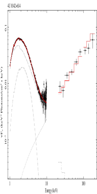
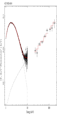
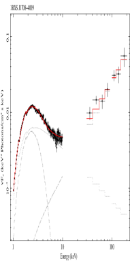
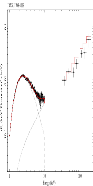
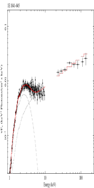
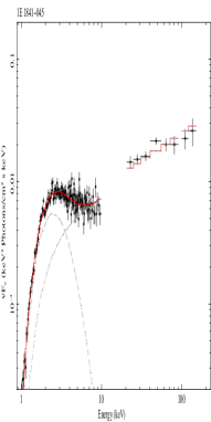
Figure 2: 4U 0142+614 , 1RXS J1708-4009   and 1E 1841-045 : left column shows the spectra in Counts/s/keV while in the right column we report the $\nu$F_ν plots. For 4U 0142+614   and 1RXS J1708-4009   the upper panels are relative to the modeling with a blackbody plus two power-laws (BB+2PL), while we used a blackbody plus power-law for 1E 1841-045 . Bottom panels report for all the sources the resonant cyclotron scattering plus a power-law model (RCS+PL). See Tab. 2 and § 4.1 for details.

Since these flux variations are rather small, we have chosen to model only the XMM–Newton   observation closest to the INTEGRAL   one (for 1RXS J1708-4009  only one XMM–Newton   observation is available though). Our results from the spectral modeling of the 1–200 keV spectrum of 4U 0142+614 , 1RXS J1708-4009 , and 1E 1841-045   are summarized in Table 2 and shown in Fig. 2.

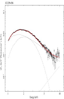
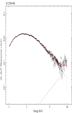
Figure 3: 1E 2259+586 : left column shows the spectra in Counts/s/keV while in the right column we report the $\nu$F_ν plots. The upper panels are relative to the modeling with a blackbody plus two power-laws (BB+2PL), while bottom panels report the resonant cyclotron scattering plus a power-law model (RCS+PL). Note the hard X-ray spectrum has been fixed at the value from Kuiper et al. (2006). See Tab. 3 and § 4.1 for details.

The case of 1E 2259+586  is rather different: it showed a large outburst (more than one order of magnitude flux increase) detected by RXTE , during which also bursting activity was detected (Kaspi et al. 2003). However, in the XMM–Newton   observations pre and post outburst, the source showed fluxes which differ only by a factor of 3 (Woods et al. 2004). Furthermore, it was observed to emit up to $\sim$30 keV by the HEXTE instrument on board of RXTE   (Kuiper et al. 2006) and by INTEGRAL , but unfortunately it is too faint in the latter observation to extract a spectrum. We then decided to model only the deepest XMM–Newton   observation taking into account of the $>$10 keV component by adding a power-law with photon index fixed at the HEXTE value (Kuiper et al. 2006). This is because sizable residuals are present at the highest energies when the XMM–Newton  spectrum is modeled either with the BB+PL or the RCS model. A satisfactory fit requires, in both cases, the addition of a hard X-ray power-law component (see also Table 3 and Fig. 3).

Summarizing, the only source that can be considered (so far) a genuine “steady” X-ray emitter, among the AXPs with hard X-ray emission is 1E 1841-045 . It is interesting to note that this is also the only AXP for which a blackbody plus a single power-law reproduces well the entire 1-200 keV spectrum, while for the other hard X-ray emitting AXPs two power-laws are required. In this respect, the spectral distribution of 1E 1841-045  resembles the one of the SGRs (see also §5).

In all cases we found that $N_{H}$, as derived from the RCS model, is lower than (or consistent with) that inferred from the BB+2PL fit (or BB+PL in the case of 1E 1841-045 ), and consistent with what derived from fitting the single X-ray edges of 4U 0142+614 , 1E 2259+586 , and 1RXS J1708-4009 (Durant & van Kerkwijk 2006). This is not surprising, since the power-law usually fitted to magnetar spectra in the soft X-ray range is well known to cause an overestimate in the column density The surface temperature we derived fitting the RCS model is systematically lower than the corresponding BB temperature in the BB+2PL or BB+PL models, and is consistent with being the same ($\sim 0.33$ keV) in the four sources. On the other hand the thermal electron velocity and the optical depth are in the ranges 0.2–0.4 and 1.0–2.1, respectively. Concerning the hard X-ray power-law, we find that the photon index is, within the errors, the same when fitting the RCS or the BB+2PL or BB+PL models (note that for 1E 2259+586   it was kept fixed), while the hard PL normalization is larger in the RCS case with respect to the BB+2PL model. Both the soft and the hard X-ray fluxes of all these AXPs derived from the RCS fitting are consistent with those implied by the usual BB+2PL fitting.

4.2 AXPs: the “transients”

“Transient” AXPs have been discovered only very recently, when an increase in the X-ray flux by a factor $\sim 100$ over the value measured a few years before was observed in XTE J1810-197   (Ibrahim et al. 2004; Gotthelf et al. 2004). Later on, new TAXPs have been observed showing large flux and spectral variations, e.g. CXOU J1647-4552   (Muno et al. 2007) and 1E 1547.0-5408   (Gelfand & Gaensler 2007; Camilo et al. 2007a; Halpern et al. 2007). Very intriguing is the discovery of pulsed radio emission correlated with the outbursts of XTE J1810-197   and 1E 1547.0-5408  (Camilo et al. 2006, 2007a), while so far only upper limits have been set on the radio emission from CXOU J1647-4552 , 1E 1048-5937   and other AXPs (Burgay et al. 2006, 2007; Camilo et al. 2007b).

It is not clear whether AXPs and TAXPs are indeed two distinct groups of sources. During the past few years it has became increasingly evident that flux variations of different magnitudes also occur in “steady” AXPs, possibly related to their bursting and glitching activity (see §4.1). Furthermore, bursts have been observed also during the outbursts of the TAXP XTE J1810-197   (Woods et al. 2005) and CXOU J1647-4552  (Muno et al. 2007), the latter also showing a large glitch (Israel et al. 2007b). However, in this paper we maintain the distinction between TAXPs and AXPs, partly for historical reasons, and partly because the two classes may indeed have different spectral properties, with the TAXPs being characterized by much softer X-ray spectra, and by the lack, so far, of detection at energies $>10$ keV.

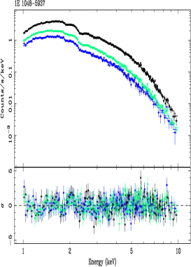
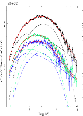
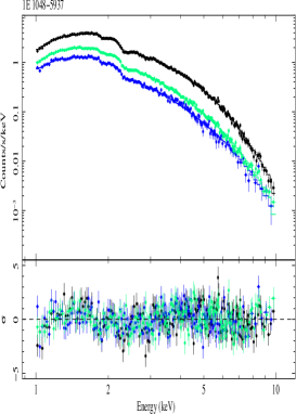
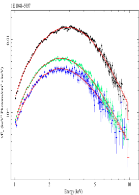
Figure 4: 1E 1048-5937 : left column represents the spectra in Counts/s/keV while in the right column we report the $\nu$F_ν plots. The upper panels are relative to the modeling with a blackbody plus one power-law (BB+PL), while bottom panels report the resonant cyclotron scattering model (RCS). See Tab. 4 and § 4.2 for details. Black, blue, and light-green colors are relative to observations taken in 2007, 2005 and 2003, respectively. The red lines represent the total model, while the dashed lines are the single components.

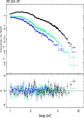
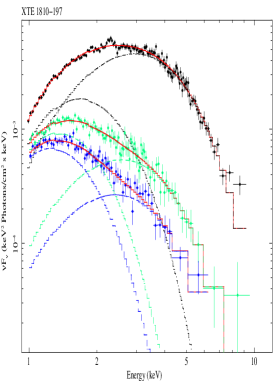
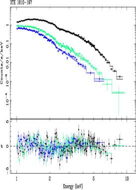
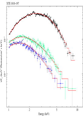
Figure 5: XTE J1810-197 : left column represents the spectra in Counts/s/keV while in the right column we report the $\nu$F_ν plots. The upper panels are relative to the modeling with two absorbed blackbodies (BB+BB), while bottom panels report the resonant cyclotron scattering model (RCS). See also Tab. 5 and § 4.2 for details. Black, light-green and blue colors are relative to observations taken on 2004, 2005 and 2006, respectively. The red lines represent the total model, while the dashed lines are the single components.

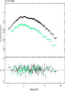
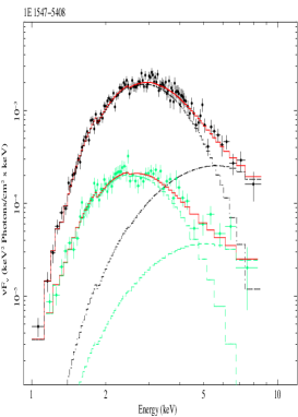
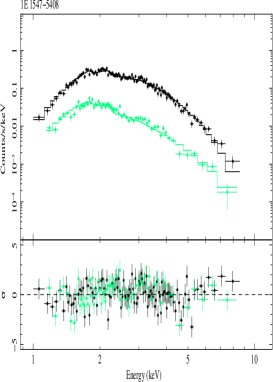
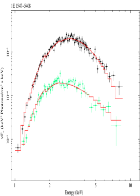
Figure 6: 1E 1547.0-5408 : left column represents the spectra in Counts/s/keV while in the right column we report the $\nu$F_ν plots. The upper panels are relative to the modeling with two blackbodies (BB+BB), while bottom panels report the resonant cyclotron scattering model (RCS). See also Tab. 6 and § 4.2 for details. Black and light-green colors are relative to observations taken on 2007 and 2006, respectively. The red lines represent the total model, while the dashed lines are the single components.

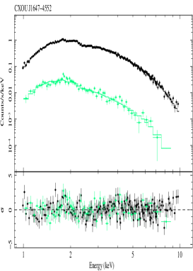
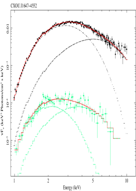
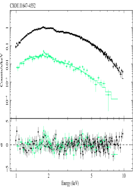
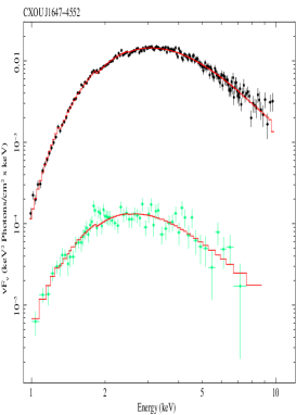
Figure 7: CXOU J1647-4552 : left column represents the spectra in Counts/s/keV while in the right column we report the $\nu$F_ν plots. The upper panels are relative to the modeling with two absorbed blackbodies (BB+BB), while bottom panels report the resonant cyclotron scattering model (RCS). See also Tab. 7 and § 4.2 for details. Black and light-green colors are relative to observations taken on 2006 September 22 and 16, respectively. The red lines represent the total model, while the dashed lines are the single components.

The results of the TAXPs spectral modeling are summarized in Tables  4, 5, 6, 7, and shown in Figs.  4, 5, 6, 7. Also in this case, we chose to model up to three spectra representative of the flux and spectral variability of these sources. Again, $N_{H}$ derived with the RCS model is lower than (or consistent with) that inferred from the more common BB+BB fitting for XTE J1810-197 , CXOU J1647-4552 , and 1E 1547.0-5408 , and significantly lower in the case of the BB+PL model applied to 1E 1048-5937   (and consistent with that derived by Durant & van Kerkwijk 2006). We also found that the RCS model can easily account for all the spectral and intensity changes in the TAXPs. With the exception of XTE J1810-197 , the surface temperature we derive for all the TAXPs is lower than, or consistent with, that of the blackbody in the BB+PL or BB+BB model (for the BB+BB model, we refer to the BB with the lowest temperature). However, considering only the RCS model, it is evident for XTE J1810-197 , 1E 1547.0-5408 , and CXOU J1647-4552   that the outburst state has a high surface temperature which cools down during the decay, while for 1E 1048-5937   this trend is less clear. Furthermore, for all the TAXP but CXOU J1647-4552 , $\beta_{T}$ increases during the outburst decay. The behavior of $\tau_{res}$ is less homogeneous: this parameter decreases with decaying flux in XTE J1810-197 and 1E 1048-5937 , remains qconstant in 1E 1547.0-5408 , and shows an increase during the outburst decay in the case of CXOU J1647-4552 . Also for these transient sources, the fluxes derived by the empirical model and the RCS model are consistent.

4.3 SGRs

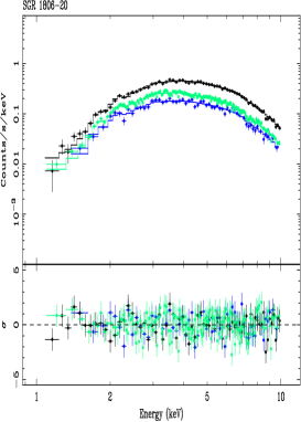
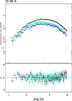
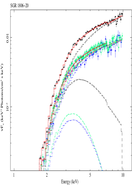
Figure 8: SGR 1806-20 : left column shows the spectra in Counts/s/keV while in the right column we report the $\nu$F_ν plots. The upper panels are relative to the modeling with a blackbody plus power-law (BB+PL), while bottom panels report the resonant cyclotron scattering model plus power-law (RCS+PL). See also Tab. 8 and §4.3 for details. Light green, black and blue colours are relative to observations taken on 2003, 2004 and 2005, respectively. The red lines represent the total model, while the dashed lines are the single components.

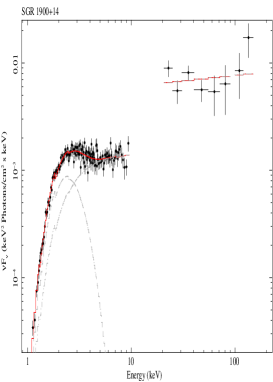
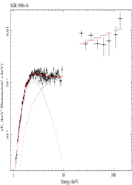
Figure 9: SGR 1900+14 : left column shows the spectra in Counts/s/keV while in the right column we report the $\nu$F_ν plots. The upper panels are relative to the modeling with a blackbody plus power-law (BB+PL), while bottom panels report the resonant cyclotron scattering model plus power-law (RCS+PL). See also Tab. 9 and §4.3 for details. The red lines represent the total model, while the dashed lines are the single components.

Finally, we consider the 1–10 keV and 1–200 keV emission of SGR 1806-20  (see Table 8 and Fig. 8) and SGR 1900+14  (see Table 9 and Fig. 9), respectively. It has been already noticed that the hard X-ray emission of SGRs is quite different from that of AXPs (see §4.1). In fact, with the exception of 1E 1841-045 , the spectra of AXPs show a clear turnover between 10 and 20 keV (see Fig. 2) and the fit requires an additional spectral component. Instead, the hard X-ray emission of SGRs seems the natural continuation of the non-thermal component which is dominant in the 1–10 keV energy range. This is why we can use a BB (or RCS) plus a single power-law in the entire 1–200 keV range for SGR 1900+14 , while for the hard X-ray emitting AXPs we were forced to add a second power-law to the BB+PL model.

Similar considerations hold for SGR 1806-20 , in which case we model the 1–10 keV emission by adding a power-law component which is intended to account for the contribution of the hard X-ray emission in the soft X-ray range. For the latter SGR we modeled three X-ray observations taken before and after the Giant Flare of 2004 December 27 (Hurley et al. 2005; Palmer et al. 2005). We found that the $N_{H}$ value is consistent within 1 $\sigma$ between the BB+PL and the RCS+PL models, and the power-law contribution and the photon index vary among the three spectra in a similar fashion for the two models. Also, in the RCS+PL model the surface temperature remains constant within the errors until before the Giant Flare, and then becomes very low after one year. Besides the temperature, the spectral variability is accounted for by changes in the parameters describing the magnetospheric currents, with $\beta_{T}$ and $\tau_{res}$ varying in the ranges 0.14–0.5 and in the 2.2–4.3, respectively.

In the SGR 1900+14   1–200 keV spectrum, we found consistent $N_{H}$ and spectral index values between the BB+PL and RCS+PL models, and a RCS surface temperature significantly lower than the corresponding BB temperature. In all the SGR observations, the derived fluxes are consistent among the two models.

5 Discussion

Before discussing our results and the physics we can derive from our model, we would like to stress once again that the RCS model involves a number of simplifications (see §2.1). One is the assumption of a single temperature surface emission. Current-carrying charges will hit and heat the star surface, generally inhomogeneously (TLK). In addition, the emission emerging from the surface is likely to be non-Plankian. While the presence of an atmosphere on top the crust of a magnetar remains a possibility (see Güver et al. 2007a,b), its properties, are then likely different from those of a standard (in radiative and hydrostatic equilibrium) atmosphere on, e.g., a canonical isolated cooling neutron star (see e.g. Ho & Lai 2003; van Adelsberg & Lai 2006). The extreme field and (relatively) low surface temperature ($\lesssim 0.5\ {\rm keV}$) of magnetar candidates may also be suggestive of a condensed surface, at least if the chemical composition is mainly Fe (see Turolla, Zane & Drake 2004). In the light of these considerations, and in the absence of a detailed model for the surface emission, and for the atmosphere of strongly magnetized NSs constantly hit by returning currents, we restricted ourself to a blackbody approximation for the seed thermal photons.

In spite of these simplifications, we find that the RCS model can describe the soft X-ray portion of the whole set of magnetar spectra we have considered, including the TAXPs variability, by using only three free parameters (plus a normalization factor). This is the same number of degrees of freedom required by the blackbody plus power law model, commonly used to fit this energy band.

5.1 Magnetar magnetospheric properties

One of the most interesting outcomes of our analysis is the measure of the magnetospheric properties of magnetars. In all sources, steady and variable ones, the value of $\tau_{res}$ is in the range of $\sim 1$–$6$. This suggests that the entire class of sources are characterized by similar properties of scattering electrons, their density and their (thermal) velocity spread. An optical depth $\tau_{0}=\tau_{res}/2$ requires a particle density $n_{e}$ (see eq. [3]) which can be easily inferred considering:

$$\tau_{0}\approx 1.8\times 10^{-20}n_{e}r_{sc}\left(\frac{1\,{\rm keV}}{\hbar\omega_{B}}\right)\,,$$ (5)

where $r_{sc}$ is the radius of the scattering sphere

$$r_{sc}\approx 8R_{NS}\left(\frac{B}{B_{crit}}\right)^{1/3}\left(\frac{1\,{\rm keV}}{\hbar\omega_{B}}\right)^{1/3}\,,$$ (6)

$R_{NS}$ is the neutron star radius and $B_{crit}\approx 4.4\times 10^{13}$ G is the quantum critical field. By taking a typical photon energy of $\sim 1\ {\rm keV}$, $R_{NS}\sim 10^{6}$ cm and $B\sim 10B_{crit}$, we get $n_{e}\approx 1.5\times 10^{13}\tau_{res}\,{\rm cm}^{-3}$. This is several orders of magnitude larger than the Goldreich-Julian density (Goldreich & Julian 1969) at the same distance, $n_{GJ}\approx n_{e}\pi r_{sc}/(3\tau_{res}R_{lc})\sim 2\times 10^{10}$ cm^-3 (where $R_{lc}$ is the light cylinder radius and we took $P\sim 10$ s). While the charge density is large when compared with the minimal Goldreich-Julian density, it provides a negligible optical depth to non-resonant Thomson scattering. Only the resonant cyclotron scattering makes an efficient photon boosting possible.

Our present model does not include a proper treatment of magnetospheric currents, so that $\tau_{res}$ is a free parameter related to the electron density. Nevertheless, it is useful to compare the values of the optical depth inferred here to those expected when a current flow arises because a steady twist is implanted in the star magnetosphere, as in the case investigated by TLK under the assumption of axysimmetry and self-similarity. If the scattering particles have a collective motion (bulk velocity $\beta_{bulk}$), the efficiency of the scattering process is related to $\tau_{res}\beta_{bulk}$ (e.g. Nobili, Turolla & Zampieri 1993). This quantity is shown as a function of the magnetic colatitude in Fig. 5 of TLK for different values of the twist angle, $\Delta\phi_{N-S}$. By assuming $\beta_{bulk}=1$ and integrating over the angle, we get the average value of the scattering depth as a function of $\Delta\phi_{N-S}$, which is shown in Fig. 10. The curves corresponding to a different value of $\beta_{bulk}$ can be obtained simply by reading the quantity shown in Fig. 10 as $\tau_{res}\beta_{bulk}$ and by rescaling the $y$-axis. As we can see, a value of $\tau_{res}\sim 1$ is only compatible with very large values of the twist angle (i.e $\Delta\phi_{N-S}>3$), while typical values of $\tau_{res}\sim 2$, as those obtained from some of our fits, require $\beta_{bulk}\lesssim 0.5$ to be compatible with $\Delta\phi_{N-S}\sim 3$ (the smaller is $\beta_{bulk}$, the smaller is the value of the twist angle). This is consistent with the fact that the RCS model has been computed under the assumption of vanishing bulk velocity for the magnetospheric currents, and it is compatible with TLK model only when in the latter it is $\beta_{bulk}\ll 1$.

5.2 Comparison between AXPs and SGRs

In the last few years the detection of bursts from AXPs (Gavriil et al. 2002; Kaspi et al. 2003) strengthened their connection with SGRs. However, the latter behave differently in many respects. Below $\sim 4$ keV, the SGRs emission can be described either by a blackbody or an RCS component. At higher energies though ($>4$ keV), their spectra require the addition of a power-law component, which well describes the spectrum until $\sim 200$ keV. The non-thermal component dominates their spectra to the point that the choice of a blackbody or the RCS model at lower energies does not affect significantly the value of the hard X-ray power-law index, nor the energy at which this component starts to dominate the spectrum (see e.g Tab. 9 and Fig. 9). The spectra of SGRs are then strongly non-thermally dominated in the 4–200 keV range.

The case of the AXPs is different (with the exception of 1E 1841-045 , see below). These sources show a more complex spectrum, with an evident non-thermal component below $\sim 10$ keV, apparently different from that observed at higher energies. For the AXPs detected at energies $>$20 keV, the spectrum can be described by a RCS component until 5–8 keV, above which the non-thermal hard X-ray component becomes important, and (e.g. for 1RXS J1708-4009   and 4U 0142+614 ) dominates until $\sim 200$ keV. In the case of the BB+2PL model instead, the non-thermal component responsible for the hard X-ray part of the spectrum starts to dominate only above $\sim 10$ keV (see e.g. Figs. 2 and 3). This is important, because the measurement of a down-break of the hard X-ray power-law has remarkable physical implications and may prove useful in constraining the physical parameters of the model for the hard X-ray emission. It is worth noting that the photon index of the hard X-ray component in AXPs does not strongly depend on the modeling of the spectrum below 10 keV, while, its normalization and, as a consequence, the value at which the hard tail starts to dominate the spectrum, do.

In this picture 1E 1841-045   seems an exception. From the spectral point of view, 1E 1841-045  appears as the more SGR-like among the AXPs. Its multi-band spectrum can be well fitted by a BB+PL or RCS+PL model, with parameters very similar to SGRs (compare Figs. 9, 2 and Tables 9, 2). This may suggest that this source is a potential transition object between the two classes. However, at variance with the SGRs, this source seems to be the least active bursters among AXPs. Note that, at variance with the other magnetars, in the case of the two SGRs and 1E 1841-045 , our model requires two additional free parameters, with respect to the BB+PL, to account for the hard X-ray power-law.

The fact that hard X-ray spectra detected from AXPs are much flatter than those of SGRs may also suggest a possible difference in the physical mechanism that powers the hard tail in the two classes of sources. Within the magnetar scenario, Thompson & Beloborodov (2005) discussed how soft $\gamma$-rays may be produced in a twisted magnetosphere, proposing two different pictures: either thermal bremsstrahlung emission from the surface region heated by returning currents, or synchrotron emission from pairs created higher up ($\sim$ 100 km) in the magnetosphere. Moreover, a third scenario involving resonant magnetic Compton up-scattering of soft X-ray photons by a non-thermal population of highly relativistic electrons has been proposed by Baring & Harding (2007). It is interesting to note that 3D Monte Carlo simulations (Fernandez & Thompson 2007; Nobili, Turolla & Zane 2008) show that multiple peaks may appear in the spectrum. In particular, in the model by Nobili, Turolla & Zane (2008), a second “hump” may be present when up-scattering is so efficient that photons start to fill the Wien peak at the typical energy of the scattering electrons. The change in the spectral slope may be due, in this scenario, to the peculiar, “double-humped” shape of the continuum. The precise localization of the down-break is therefore of great potential importance and might provide useful information on the underlying physical mechanism responsible for the hard emission.

The RCS model applied to the evolution of the outbursts of the TAXPs known up to now shows how the outburst may results from a heating of the NS surface, which slowly cools in a timescale of months/years. AXPs outbursts are thought to be caused by large scale rearrangement of the surface/magnetospheric field, either accompanied or triggered by fracturing of the NS crust. It is worth noticing that from our modeling we find that the surface temperature cools down during the outburst decay, while the magnetospheric characteristics change in a different way from source to source.

5.3 Correlations

The quite large number of observations we analyzed (both relative to different sources and to single sources in different emission states) allows to search for possible correlations among the various quantities, both in the entire sample, i.e. looking at the population of magnetar candidates at large, and in the time evolution of a single source.

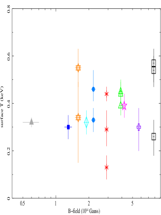
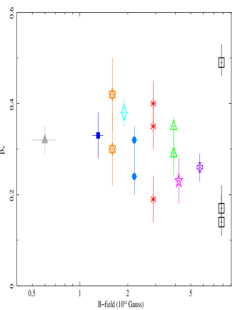
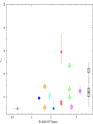
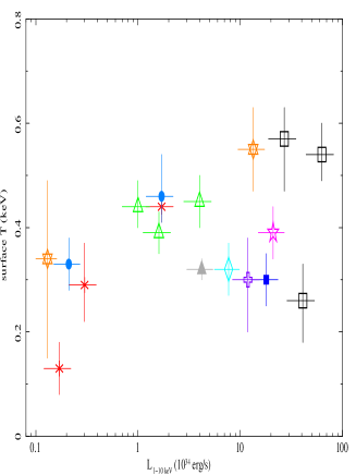
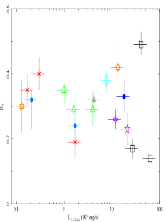
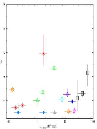
Figure 11: Comparison between the derived spectral parameters and the sources’ properties (see §5 for details). To infer the 1–10 keV luminosity we assumed a distance of 3, 3, 5, 3.3, 3, 7, 10, 4, 5, and 10 kpc, for the sources ordered as the labels reported in the top panel (from left to right and top to bottom). Errors in the luminosities are assumed to be 30% of the reported values (which is of the order of the flux errors), although the real error (including that on the distance) is actually much larger.

Fig. 11 summarizes the results of our spectral fits. The various panels show how the three model parameters ($T$, $\tau_{res}$ and $\beta_{T}$) are related to the X-ray luminosity in the 1–10 keV band ($L_{\rm 1-10\,keV}$) and to the magnetic field $B$. The latter is derived from $P$ and $\dot{P}$, assuming that the magnetic field is a core-centered dipole and the spin-down is due magnetic dipole radiation.

An inspection of the panels in Fig. 11 does not reveal any obvious correlation for the entire set of observations. To verify this, we have run a Spearman rank test and we only found a positive correlation between $B$ and both $\tau_{res}$ and $\beta_{T}$ (deviation from the null hypothesis at about the $93\%$ and $89\%$ confidence level, respectively). No correlations with a significance level above $\sim 65\%$ were found in all the other cases. Both parameters $\beta_{T}$ and $\tau_{res}$ control the scattering efficiency, but the meaning of their correlation with the field strength, which seems to be direct in the case of the optical depth and inverse in the case of the thermal velocity (Fig. 11) is not of immediate interpretation. The optical depth scales as $n_{e}r/B$ (see eq. [3]). If we make again a comparison with the twisted magnetosphere model (TLK), in which $n_{e}\propto B/r$, this is not expected. Taken face value, an increase of the optical depth with increasing $B$ implies that the product $n_{e}r$ grows more rapidly than $B$. Since both in the RCS model and in TLK the scattering radius is $\propto B^{1/3}$, this implies that $n_{e}$ should grow faster than what expected in a self-similar magnetostatic configuration. Furthermore, it is interesting to note

On the other, we caveat that these considerations are largely model dependent and, in order to assess this issue, a detailed treatment of the magnetosphere, including more realistic profiles for the electron density and velocity distribution, is needed.

As discussed earlier, a more interesting trend is found restricting to observations of the same source at different epochs. In many transient AXPs (e.g. XTE J1810-197 , 1E 1547.0-5408 , and CXOU J1647-4552 ) we observe a clear correlation between the surface temperature and the X-ray luminosity, which is expected since in the RCS model an enhanced surface thermal emission produces more seeds for resonant up-scattering. However, once again there is no clear trend relating changes in $\tau_{res}$ and $\beta_{T}$ to changes in luminosity for the entire TAXP sample. In most transient sources at least one of these two parameters increases with flux, and this may be enough to guarantee that the spectrum hardens at larger luminosities, but in no case there is a simultaneous increase or decrease of both $\tau_{res}$ and $\beta_{T}$ during the outburst decay. Whether this is due to a degeneracy in the model parameter space or it reflects a real trend is not clear at present.

6 Conclusion

In this paper we showed that the soft X-ray emission of magnetars can be explained by resonant cyclotron scattering of their thermal surface emission by a cloud of hot magnetospheric electrons. This model satisfactorily reproduces the spectral shape of all magnetars soft X-ray emission, using the same number of free parameters than the widely used blackbody plus power-law model (except for the SGRs where the much harder spectrum below 10 keV, still requires the addition of a power-law on top of the resonant cyclotron scattering model, being the same power-law component responsible for their hard X-ray emission). This means that the RCS model not only catches the main features of the thermal and non-thermal components observed in these sources below $\sim 10$ keV, but also successfully provides a quantitative interpretation. For the magnetars presenting an hard X-ray emission we included this further component in order to take into account in our modeling of the contribution of this component down to the soft X-ray part of the spectrum.

This work represents one of the first attempts to infer some physical values from the $1-10$ keV spectra of magnetars. Future refinements are in progress, in order to improve the RCS model from a 1D analytical model toward a 3D Monte Carlo based code (as the more advanced codes developed by Fernandez & Thompson 2007 and Nobili, Turolla & Zane 2008). Furthermore, this model eventually applied to the detailed spectra that XEUS and/or Con–X will possibly make available in the near future, appear a promising step toward the complete understanding of the physics behind magnetars soft X-ray emission.

We acknowledge Valentina Bianchin and Gavin Ramsay for their help in building the XSPEC RCS model, and Fotis Gavriil for kindly allowing us to look into his preliminary model. Furthermore, we thank Gianluca Israel and Andrea Tiengo for useful discussions and key comments on the preliminary draft. NR is supported by an NWO Veni Fellowship, and acknowledges the warm hospitality of the Mullard Space Science Laboratory, where this work was started, and of the Purdue University where it has been completed. SZ acknowledges STFC for support through an Advanced Fellowship. D.G. acknowledges the French Space Agency (CNES) for financial support. This paper is based on observations obtained with XMM–Newton  and INTEGRAL , which are both ESA science missions with instruments and contributions directly funded by ESA Member States and the USA (through NASA). The RCS model is available to the community on the XSPEC website.

Table 1: Log Of The XMM–Newton   and INTEGRAL   Observations Analysed In This Paper.

XMM–Newton
Source	Date (YYYY/MM/DD)	Exposure (ks)
4U 0142+614	2004/03/01	44
1RXS J1708-4009	2003/08/28	45
1E 1841-045	2002/10/07	6
1E 2259+586	2002/06/11	52
1E 1048-5937	2003/06/16	69
	2005/06/17	32
	2007/06/14	48
XTE J1810-197	2004/09/18	28
	2005/09/20	42
	2006/03/13	51
1E 1547.0-5408	2006/08/21	47
	2007/08/09	16
CXOU J1647-4552	2006/09/16	80
	2006/09/22	20
SGR 1806-20	2003/04/03	55
	2004/10/06	19
	2005/10/04	33
SGR 1900+14	2005/09/17	30
INTEGRAL
Source	Date (YYYY/MM/DD)	Exposure (Ms)
4U 0142+614	2003/03/03-2006/08/13	1.9
1RXS J1708-4009	2003/02/28-2005/10/02	2.7
1E 1841-045	2003/03/10-2006/04/28	4.0
SGR 1900+14	2003/03/06-2006/09/26	3.7

Figure 1: Distorsion of a seed blackbody spectrum through resonant cyclotron scattering onto magnetosferic electrons, for two values of the blackbody temperature, 0.2 keV and 0.8 keV. Black lines show the RCS model for $\beta_{T}=0.2$ and $\tau_{res}=$ 2, 4, 8 (from bottom to top), while grey lines are relative to $\beta_{T}=0.4$ and $\tau_{res}=$ 2, 4, 8 (from bottom to top). The normalizations of the various curves are arbitrary.

Table 2: Spectral Parameters: 4U 0142+614 , 1RXS J1708-4009 , and 1E 1841-045 

AXPs	4U 0142+614∗		1RXS J1708–4009∗		1E 1841–045
Parameters	BB+2PL	RCS+PL	BB+2PL	RCS+PL	BB+PL	RCS+PL
NH	1.67${}^{+0.02}_{-0.02}$	0.81${}^{+0.05}_{-0.05}$	1.91${}^{+0.06}_{-0.06}$	1.67${}^{+0.05}_{-0.05}$	2.38${}^{+0.4}_{-0.1}$	2.57${}^{+0.13}_{-0.15}$
constant	1.01	1.10	1.05	0.80	1.02	1.09
kT (keV)	0.43${}^{+0.03}_{-0.03}$	0.30${}^{+0.05}_{-0.05}$	0.47${}^{+0.01}_{-0.01}$	0.32${}^{+0.05}_{-0.05}$	0.51${}^{+0.03}_{-0.02}$	0.39${}^{+0.05}_{-0.05}$
BB norm	8.7${}^{+0.4}_{-0.5}\times 10^{-4}$		2.4${}^{+0.1}_{-0.2}\times 10^{-4}$		2.4${}^{+0.6}_{-0.3}\times 10^{-4}$
$\Gamma_{1}$	4.14${}^{+0.04}_{-0.04}$		2.70${}^{+0.08}_{-0.08}$
PL1 norm	0.30${}^{+0.08}_{-0.08}$		0.016${}^{+0.003}_{-0.004}$
$\beta_{T}$		0.33${}^{+0.05}_{-0.05}$		0.38${}^{+0.03}_{-0.03}$		0.23${}^{+0.05}_{-0.05}$
$\tau_{res}$		1.9${}^{+0.2}_{-0.2}$		2.1${}^{+0.2}_{-0.2}$		1.13${}^{+0.3}_{-0.2}$
RCS norm		4.5${}^{+0.6}_{-0.8}\times 10^{-3}$		8.1${}^{+1.1}_{-1.3}\times 10^{-4}$		3.1${}^{+2.3}_{-1.1}\times 10^{-4}$
$\Gamma_{2}$	0.78${}^{+0.1}_{-0.07}$	1.1${}^{+0.1}_{-0.1}$	0.76${}^{+0.1}_{-0.1}$	1.0${}^{+0.1}_{-0.1}$	1.47${}^{+0.04}_{-0.05}$	1.47${}^{+0.05}_{-0.05}$
PL2 norm	1.4${}^{+0.1}_{-0.1}\times 10^{-4}$	5.0${}^{+0.1}_{-0.1}\times 10^{-4}$	8.6${}^{+0.1}_{-0.1}\times 10^{-5}$	4.2${}^{+0.1}_{-0.1}\times 10^{-4}$	2.4${}^{+0.6}_{-0.6}\times 10^{-3}$	2.2${}^{+0.1}_{-0.1}\times 10^{-3}$
Flux 1–10 keV	1.1${}^{+0.8}_{-0.8}\times 10^{-10}$	1.1${}^{+0.8}_{-0.8}\times 10^{-10}$	2.6${}^{+0.3}_{-0.3}\times 10^{-11}$	2.6${}^{+1.1}_{-0.8}\times 10^{-11}$	2.2${}^{+0.2}_{-0.3}\times 10^{-11}$	2.1${}^{+0.2}_{-0.3}\times 10^{-11}$
Flux 1–200 keV	2.3${}^{+1.7}_{-1.1}\times 10^{-10}$	2.3${}^{+1.0}_{-1.3}\times 10^{-10}$	1.1${}^{+0.5}_{-0.5}\times 10^{-10}$	1.4${}^{+0.8}_{-0.8}\times 10^{-10}$	1.1${}^{+0.8}_{-0.8}\times 10^{-10}$	1.1${}^{+0.8}_{-0.6}\times 10^{-10}$
$\chi^{2}_{\nu}$ (dof)	0.99 (216)	0.80 (216)	1.11 (202)	1.01 (202)	1.14 (158)	1.08 (156)

Table 3: Spectral Parameters: 1E 2259+586 

AXP	1E 2259+586∗
Parameters	BB+2PL	RCS+PL
NH	0.97${}^{+0.04}_{-0.03}$	0.89${}^{+0.02}_{-0.02}$
kT (keV)	0.41${}^{+0.03}_{-0.03}$	0.32${}^{+0.02}_{-0.02}$
BB norm	2.77${}^{+0.02}_{-0.01}\times 10^{-4}$
$\Gamma_{1}$	3.98${}^{+0.03}_{-0.02}$
PL1 norm	4.89${}^{+0.04}_{-0.04}\times 10^{-2}$
$\beta_{T}$		0.32${}^{+0.03}_{-0.03}$
$\tau_{res}$		1.0${}^{+0.2}_{-0.2}$
RCS norm		1.0${}^{+0.1}_{-0.1}\times 10^{-3}$
$\Gamma_{2}$	1.02	1.02
PL2 norm	1.65${}^{+1.0}_{-1.0}\times 10^{-7}$	5.0${}^{+1.0}_{-1.0}\times 10^{-5}$
Flux 1–10 keV	2.5${}^{+0.1}_{-0.1}\times 10^{-11}$	2.5${}^{+0.1}_{-0.1}\times 10^{-11}$
$\chi^{2}_{\nu}$ (dof)	1.15 (178)	0.94 (178)

Table 4: Spectral Parameters: 1E 1048-5937 

AXP	1E 1048-5937
	2003		2005		2007
Parameters	BB+PL	RCS	BB+PL	RCS	BB+PL	RCS
NH	1.68${}^{+0.03}_{-0.03}$	0.98${}^{+0.04}_{-0.04}$	1.56${}^{+0.05}_{-0.04}$	0.73${}^{+0.04}_{-0.04}$	1.71${}^{+0.04}_{-0.03}$	0.82${}^{+0.05}_{-0.05}$
kT (keV)	0.63${}^{+0.02}_{-0.02}$	0.39${}^{+0.04}_{-0.04}$	0.64${}^{+0.03}_{-0.04}$	0.44${}^{+0.05}_{-0.04}$	0.73${}^{+0.01}_{-0.01}$	0.45${}^{+0.05}_{-0.05}$
BB norm	1.01${}^{+0.05}_{-0.05}\times 10^{-4}$		0.7${}^{+0.1}_{-0.1}\times 10^{-4}$		3.00${}^{+0.08}_{-0.08}\times 10^{-4}$
$\Gamma_{1}$	3.31${}^{+0.02}_{-0.04}$		3.18${}^{+0.03}_{-0.04}$		3.20${}^{+0.07}_{-0.07}$
PL1 norm	1.10${}^{+0.13}_{-0.04}\times 10^{-2}$		0.7${}^{+0.1}_{-0.2}\times 10^{-2}$		2.2${}^{+0.1}_{-0.1}\times 10^{-2}$
$\beta_{T}$		0.29${}^{+0.02}_{-0.02}$		0.35${}^{+0.02}_{-0.04}$		0.29${}^{+0.05}_{-0.05}$
$\tau_{res}$		2.7${}^{+0.2}_{-0.4}$		2.0${}^{+0.1}_{-0.5}$		4.7${}^{+0.2}_{-0.2}$
RCS norm		1.9${}^{+0.1}_{-0.1}\times 10^{-4}$		1.01${}^{+0.08}_{-0.11}\times 10^{-4}$		3.0${}^{+0.1}_{-0.1}\times 10^{-4}$
Flux 1–10 keV	1.1${}^{+0.4}_{-0.4}\times 10^{-11}$	1.1${}^{+0.4}_{-0.4}\times 10^{-11}$	0.8${}^{+0.3}_{-0.4}\times 10^{-11}$	0.8${}^{+0.4}_{-0.4}\times 10^{-11}$	3.0${}^{+0.5}_{-0.4}\times 10^{-11}$	3.0${}^{+0.7}_{-0.6}\times 10^{-11}$
$\chi^{2}_{\nu}$ (dof)	0.99 (176)	0.98 (176)	0.99 (153)	1.00 (153)	1.08 (184)	1.23 (184)

Table 5: Spectral Parameters: XTE J1810-197 

AXP	XTE J1810-197
	2004		2005		2006
Parameters	BB+BB	RCS	BB+BB	RCS	BB+BB	RCS
NH	0.58${}^{+0.06}_{-0.05}$	0.40${}^{+0.05}_{-0.05}$	0.52${}^{+0.08}_{-0.07}$	0.25${}^{+0.05}_{-0.05}$	0.4${}^{+0.1}_{-0.1}$	0.14${}^{+0.22}_{-0.05}$
kT1 (keV)	0.36${}^{+0.02}_{-0.02}$	0.44${}^{+0.03}_{-0.03}$	0.27${}^{+0.03}_{-0.02}$	0.29${}^{+0.08}_{-0.07}$	0.25${}^{+0.03}_{-0.04}$	0.13${}^{+0.05}_{-0.05}$
BB1 norm	6.6${}^{+0.5}_{-0.4}\times 10^{-5}$		3.8${}^{+0.2}_{-0.1}\times 10^{-5}$		2.7${}^{+0.3}_{-0.3}\times 10^{-5}$
kT2 (keV)	0.71${}^{+0.01}_{-0.02}$		0.58${}^{+0.03}_{-0.03}$		0.36${}^{+0.05}_{-0.07}$
BB2 norm	12${}^{+1}_{-1}\times 10^{-5}$		1.5${}^{+0.1}_{-0.1}\times 10^{-5}$		0.7${}^{+0.1}_{-0.1}\times 10^{-5}$
$\beta_{T}$		0.19${}^{+0.05}_{-0.05}$		0.40${}^{+0.05}_{-0.05}$		0.35${}^{+0.05}_{-0.05}$
$\tau_{res}$		5.9${}^{+1.6}_{-1.0}$		1.6${}^{+0.2}_{-0.2}$		1.4${}^{+0.1}_{-0.1}$
RCS norm		1.1${}^{+0.3}_{-0.3}\times 10^{-4}$		7.2${}^{+0.3}_{-0.4}\times 10^{-5}$		2.5${}^{+0.5}_{-0.5}\times 10^{-4}$
Flux 1–10 keV	12${}^{+3}_{-2}\times 10^{-12}$	11${}^{+3}_{-3}\times 10^{-12}$	2.2${}^{+0.1}_{-0.2}\times 10^{-12}$	2.1${}^{+0.2}_{-0.2}\times 10^{-12}$	1.2${}^{+0.3}_{-0.4}\times 10^{-12}$	1.2${}^{+0.5}_{-0.4}\times 10^{-12}$
$\chi^{2}_{\nu}$ (dof)	1.21 (135)	1.27 (135)	0.94 (97)	1.07 (97)	0.97 (67)	1.00 (67)

Table 6: Spectral Parameters: 1E 1547.0-5408 

AXP	1E 1547.0-5408
	2006		2007
Parameters	BB+BB	RCS	BB+BB	RCS
NH	3.76${}^{+0.06}_{-0.05}$	2.8${}^{+0.1}_{-0.1}$	4.58${}^{+0.08}_{-0.07}$	4.6${}^{+0.1}_{-0.1}$
kT1 (keV)	0.46${}^{+0.03}_{-0.02}$	0.33${}^{+0.05}_{-0.05}$	0.51${}^{+0.02}_{-0.02}$	0.46${}^{+0.08}_{-0.05}$
BB1 norm	1.2${}^{+0.5}_{-0.4}\times 10^{-5}$		7.2${}^{+0.5}_{-0.5}\times 10^{-6}$
kT2 (keV)	1.2${}^{+0.1}_{-0.1}$		1.34${}^{+0.08}_{-0.07}$
BB2 norm	1.4${}^{+0.1}_{-0.1}\times 10^{-6}$		1.4${}^{+0.1}_{-0.1}\times 10^{-4}$
$\beta_{T}$		0.32${}^{+0.03}_{-0.09}$		0.24${}^{+0.04}_{-0.04}$
$\tau_{res}$		1.0${}^{+0.8}_{-0.2}$		1.0${}^{+0.1}_{-0.1}$
RCS norm		2.6${}^{+0.3}_{-0.3}\times 10^{-5}$		9.4${}^{+0.3}_{-0.4}\times 10^{-5}$
Flux 1–10 keV	3.2${}^{+0.1}_{-0.1}\times 10^{-13}$	3.1${}^{+0.1}_{-0.2}\times 10^{-13}$	3.0${}^{+0.1}_{-0.1}\times 10^{-12}$	3.0${}^{+0.2}_{-0.2}\times 10^{-12}$
$\chi^{2}_{\nu}$ (dof)	1.18 (60)	1.20 (60)	1.02 (105)	1.13 (105)

Table 7: Spectral Parameters: CXOU J1647-4552 

AXP	CXOU J1647-4552
	2006/09/16		2006/09/22
Parameters	BB+BB	RCS	BB+BB	RCS
NH	2.14${}^{+0.06}_{-0.06}$	2.08${}^{+0.15}_{-0.16}$	2.34${}^{+0.04}_{-0.04}$	2.40${}^{+0.04}_{-0.04}$
kT1 (keV)	0.39${}^{+0.03}_{-0.02}$	0.34${}^{+0.15}_{-0.19}$	0.59${}^{+0.02}_{-0.02}$	0.55${}^{+0.08}_{-0.08}$
BB1 norm	4.5${}^{+0.5}_{-0.4}\times 10^{-6}$		4.4${}^{+0.5}_{-0.5}\times 10^{-4}$
kT2 (keV)	0.85${}^{+0.1}_{-0.1}$		1.23${}^{+0.04}_{-0.04}$
BB2 norm	2.4${}^{+0.1}_{-0.1}\times 10^{-6}$		1.4${}^{+0.1}_{-0.1}\times 10^{-4}$
$\beta_{T}$		0.30${}^{+0.08}_{-0.08}$		0.42${}^{+0.08}_{-0.08}$
$\tau_{res}$		2.9${}^{+0.1}_{-0.1}$		1.09${}^{+0.05}_{-0.05}$
RCS norm		7.8${}^{+0.3}_{-0.3}\times 10^{-6}$		3.0${}^{+0.3}_{-0.4}\times 10^{-3}$
Flux 1–10 keV	2.4${}^{+0.1}_{-0.1}\times 10^{-13}$	2.4${}^{+0.1}_{-0.1}\times 10^{-13}$	2.2${}^{+0.1}_{-0.1}\times 10^{-11}$	2.2${}^{+0.1}_{-0.1}\times 10^{-11}$
$\chi^{2}_{\nu}$ (dof)	1.00 (73)	1.23 (73)	1.01 (136)	1.06 (136)

Table 8: Spectral Parameters: SGR 1806-20 

SGR	SGR 1806-20
	2003		2004		2005
Parameters	BB+PL	RCS+PL	BB+PL	RCS+PL	BB+PL	RCS+PL
NH	9.9${}^{+0.4}_{-0.4}$	9.3${}^{+1.0}_{-0.8}$	9.7${}^{+0.2}_{-0.2}$	10.1${}^{+0.6}_{-0.8}$	10.2${}^{+1.0}_{-0.8}$	11.0${}^{+1.0}_{-1.0}$
kT (keV)	0.56${}^{+0.05}_{-0.04}$	0.57${}^{+0.06}_{-0.1}$	0.72${}^{+0.06}_{-0.07}$	0.54${}^{+0.06}_{-0.05}$	0.57${}^{+0.04}_{-0.04}$	0.26${}^{+0.07}_{-0.08}$
BB norm	5.5${}^{+0.3}_{-0.3}\times 10^{-5}$		1.0${}^{+0.4}_{-0.3}\times 10^{-4}$		7.4${}^{+0.4}_{-0.3}\times 10^{-5}$
$\beta_{T}$		0.17${}^{+0.03}_{-0.03}$		0.14${}^{+0.08}_{-0.03}$		0.49${}^{+0.04}_{-0.03}$
$\tau_{res}$		2.2${}^{+1.5}_{-1.1}$		4.3${}^{+0.7}_{-1.1}$		2.6${}^{+0.2}_{-0.3}$
RCS norm		3.8${}^{+0.5}_{-0.5}\times 10^{-5}$		7.4${}^{+0.7}_{-0.8}\times 10^{-5}$		4.6${}^{+0.7}_{-0.8}\times 10^{-4}$
$\Gamma$	1.5${}^{+0.1}_{-0.1}$	1.2${}^{+0.1}_{-0.1}$	1.3${}^{+0.1}_{-0.1}$	1.3${}^{+0.1}_{-0.1}$	1.5${}^{+0.1}_{-0.1}$	1.2${}^{+0.2}_{-0.1}$
PL norm	3.1${}^{+0.2}_{-0.2}\times 10^{-3}$	1.7${}^{+0.2}_{-0.3}\times 10^{-3}$	4.7${}^{+0.2}_{-0.2}\times 10^{-3}$	5.1${}^{+0.4}_{-0.3}\times 10^{-3}$	3.8${}^{+0.2}_{-0.3}\times 10^{-3}$	1.7${}^{+0.8}_{-1.0}\times 10^{-3}$
Flux 1–10 keV	1.2${}^{+0.5}_{-0.6}\times 10^{-11}$	1.2${}^{+0.8}_{-0.8}\times 10^{-11}$	2.6${}^{+0.6}_{-0.7}\times 10^{-11}$	2.6${}^{+0.7}_{-0.8}\times 10^{-11}$	1.4${}^{+0.5}_{-0.6}\times 10^{-11}$	1.3${}^{+0.8}_{-0.8}\times 10^{-11}$
$\chi^{2}_{\nu}$ (dof)	0.96 (54)	1.03 (52)	1.01 (65)	0.97 (63)	1.02 (159)	0.90 (157)

Table 9: Spectral Parameters: SGR 1900+14 

SGR	SGR 1900+14
Parameters	BB+PL	RCS+PL
NH	3.5${}^{+0.1}_{-0.1}$	4.0${}^{+0.1}_{-0.1}$
constant	1.20	1.10
kT (keV)	0.45${}^{+0.04}_{-0.04}$	0.30${}^{+0.08}_{-0.1}$
BB norm	6.7${}^{+0.1}_{-0.1}\times 10^{-5}$
$\beta_{T}$		0.26${}^{+0.03}_{-0.03}$
$\tau_{res}$		2.5${}^{+0.5}_{-0.2}$
RCS norm		1.8${}^{+0.04}_{-0.05}\times 10^{-4}$
$\Gamma$	1.4${}^{+0.1}_{-0.1}$	1.24${}^{+0.07}_{-0.07}$
PL norm	4.4${}^{+0.1}_{-0.1}\times 10^{-4}$	3.0${}^{+0.1}_{-0.1}\times 10^{-4}$
Flux 1–10 keV	3.9${}^{+0.1}_{-0.1}\times 10^{-12}$	3.8${}^{+0.1}_{-0.1}\times 10^{-12}$
Flux 1–200 keV	1.7${}^{+0.1}_{-0.1}\times 10^{-11}$	1.7${}^{+0.1}_{-0.1}\times 10^{-11}$
$\chi^{2}_{\nu}$ (dof)	1.18 (141)	1.15 (139)

                                       

Figure 10: Angle-averaged optical depth in a twisted magnetosphere model (Thompson Lyutikov & Kulkarni 2002) as a function of the twist angle. The curve refers to $\beta_{bulk}=1$; for different values of the bulk velocity the ordinate should be divided by $\beta_{bulk}$.

References

- (1) Anders, E. & Grevesse, N., 1989, Geochimica & Cosmochimica Acta 53, 197
- (2) Balucinska-Church, M. & McCammon, D. 1992, ApJ, 400, 699
- (3) Beloborodov, A. M. & Thompson, C. 2007, ApJ, 657, 967
- (4) Burgay, M., Rea, N., Israel, G. L., Possenti, A., Burderi, L., di Salvo, T., D’Amico, N., Stella, L. 2006, MNRAS, 372, 410
- (5) Burgay, M., Rea, N., Israel, G. L., Possenti, A. 2007, ATel, # 903
- (6) Campana, S., Rea, N., Israel, G. L., Turolla, R., Zane, S., 2007, A&A, 463, 1047
- (7) Chatterjee, P., Hernquist, L., & Narayan, R., 2000, ApJ, 534, 373
- (8) Camilo, F., Ransom, S. M., Halpern, J. P., Reynolds, J., Helfand, D. J.; Zimmerman, N., Sarkissian, J. 2006, Nature, 442, 892
- (9) Camilo, F., Ransom, S. M., Halpern, J. P., Reynolds, J. 2007a, ApJ, 666, L93
- (10) Camilo, F. & Reynolds, J., 2007b, ATel # 1056
- (11) Dall’Osso, S., Israel, G.L., Stella, L., Possenti, A., & Perozzi, E. 2003, ApJ, 499, 485
- (12) Dib, R., Kaspi, V. M., Gavriil, F. 2007a, ApJ in press, arXiv0706.4156
- (13) Dib, R., Kaspi, V. M., Gavriil, F. P., Woods, P. M. 2007b, ATel # 104
- (14) Duncan, R.C., & Thompson, C. 1992, ApJ, 392, L9
- (15) Durant, M., & van Kerkwijk, M. H., 2006, ApJ, 650, 1082
- (16) Fernandez, R., & Thompson, C., 2007, ApJ, 660, 615
- (17) Gavriil, F.P. & Kaspi, V.M. 2002, ApJ, 567, 1067
- (18) Gavriil, F.P., Kaspi V.M., & Woods, P.M. 2002, Nature, 419, 142
- (19) Gavriil, F.P. & Kaspi, V.M. 2004, ApJ, 609, L67
- (20) Gavriil, Fotis P., Kaspi, V. M., & Woods, P. M. 2006, ApJ, 641, 418
- (21) Gelfand, J. D. & Gaensler, B. M., 2007, ApJ, 667, 1111
- (22) Goldreich, P. & Julian W.H. 1969, ApJ, 157, 869
- (23) Gonzalez, M. E., Dib, R., Kaspi, V. M., Woods, P. M., Tam, C. R., Gavriil, F. P 2007, ApJ submitted (arXiv0708.2756)
- (24) Götz, D., Mereghetti, S., Tiengo, A., Esposito, P. 2006, A&A, 449, L31
- (25) Götz, D., et al. 2007, A&A, 475, 317
- (26) Gotthelf, E. V.; Halpern, J. P.; Buxton, M.; Bailyn, C, 2004, ApJ, 605, 368
- (27) Güver, T., Özel, F., Gög̈üs, E., Kouveliotou, C., 2007a, ApJ, 667, L73
- (28) Güver, T., Özel, F., & Gög̈üs, 2007b, ApJ in press (arXiv0705.3982)
- (29) Haberl, F., Freyberg, M. J., Briel, U. G., Dennerl, K., Zavlin, V. E. 2004, SPIE, 5165, 104
- (30) Haberl, F., Zavlin, V.E., Trumper, J. & Burwitz, V., 2004, A&A 419, 1077
- (31) Haberl, F. 2007, Ap&SS, 308, 73
- (32) Halpern, J. P., Gotthelf, E. V., Reynolds, J., Ransom, S. M., Camilo, F., 2007, ApJ in press (arXiv0711.3780)
- (33) Ho, W.C.G. & Lai, D. 2003, MNRAS, 338, 233
- (34) Hulleman, F., van Kerkwijk, M.H. & Kulkarni, S.R. 2000, Nature, 408, 689
- (35) Hurley, K., et al. 2005, Nature, 434, 1098
- (36) Ibrahim, A. I., et al. 2004, ApJ, 609, L21
- (37) Israel, G. L., Götz, D., Zane, S., Dall’Osso, S., Rea, N., Stella, L. 2007a, A&A, 476, L9I
- (38) Israel, G. L., Campana, S., Dall’Osso, S., Muno, M. P., Cummings, J., Perna, R., Stella, L. 2007b, ApJ, 664, 448
- (39) Jansen, F., et al. 2001, A&A, 365, L1
- (40) Kaspi, V.M., Gavriil, F.P., Woods, P.M., Jensen, J.B., Roberts, M.S.E., & Chakrabarty, D., 2003, ApJ, 588, L93
- (41) Kuiper,L., Hermsen, W., & Méndez, M. 2004, ApJ, 613, 1173
- (42) Kuiper, L., Hermsen, W., den Hartog, P. R., Collmar, W., 2006, ApJ, 645, 556
- (43) Lamb, D. Q., Wang, J. C. L. & Wasserman, I. 1990, ApJ, 363, 670
- (44) Lyutikov, M., & Gavriil F.P., 2006, MNRAS, 368, 690
- Lebrun et al. (2003) Lebrun, F., Leray, J.P., Lavocat, P., et al. 2003, A&A, 411, L141
- (46) Lodders, K. 2003, ApJ, 591, 1220
- (47) McLaughlin, M. A., et al. 2006, Nature, 439, 817
- (48) Marsden, D. & White, N. E. 2001, ApJ, 551, L155
- (49) Mereghetti, S., Tiengo, A., Stella, L., Israel, G.L., Rea, N., Zane, S., & Oosterbroek, T., 2004, ApJ, 608, 427
- (50) Mereghetti, S., et al. 2005, ApJ, 628, 938
- (51) Mereghetti, S., Götz, D., Mirabel, I. F., Hurley, K. 2005, A&A 433, L9
- Molkov et al. (2005)
- (53) Mereghetti, S., 2008, A&AR submitted (arXiv:0804.0250)
- (54) Molkov, S., Hurley, K., Sunyaev, R., et al., 2005, A&A, 433, L13
- (55) Muno, M. P., Gaensler, B. M., Clark, J. S., de Grijs, R., Pooley, D., Stevens, I. R., Portegies Zwart, S. F 2007, MNRAS, 378, L44
- (56) Nagel, W. 1981, ApJ, 251, 288
- (57) Nobili, L., Turolla, R. & Zampieri, L. 1993, ApJ, 404, 686
- (58) Nobili, L., Turolla, R. & Zane, S., 2008, MNRAS in press, arXiv:0802.2647
- (59) Palmer, D. M., et al. 2005, Nature, 434, 1107
- (60) Perna, R., Heyl, J., Hernquist, L., 2000, ApJ, 541, 344
- (61) Rea, N., et al. 2005, MNRAS, 361, 710
- (62) Rea, N., Turolla, R., Zane, S., Tramacere, A., Israel, G.L., Stella, L., Campana, R., 2007a, ApJ, 661, L65
- (63) Rea, N., Zane, S., Lyutikov, M. & Turolla, R., 2007b, Ap&SS, 308, 61
- (64) Rea, N., et al. 2007c, MNRAS, 381, 293
- (65) Strüder, L. et al. 2001, A&A, 365, L18
- (66) Tam, C. R., Gavriil, F., Dib, R., Kaspi, V. M.; Woods, P. M., Bassa, C. 2007, ApJ in press (arXiv0707.2093)
- Thompson & Belobodorov (2005) Thompson, C., & Beloborodov, A. M., ApJ 634, 565 (2005)
- (68) Thompson, C., & Duncan, R.C., 1993, ApJ, 408, 194
- (69) Thompson, C., & Duncan, R.C. 1995, MNRAS, 275, 255
- (70) Thompson, C., & Duncan, R.C. 1996, ApJ, 473, 322
- (71) Thompson, C., Lyutikov, M. & Kulkarni, S.R., 2002, ApJ, 574, 332
- (72) Turner, M. J. L. et al. 2001, A&A, 365, L27
- (73) Turolla, R., Zane, S. & Drake, J.J. 2004, ApJ, 603, 265
- Ubertini et al. (2003) Ubertini, P., et al. 2003, A&A 411, L131
- (75) van Adelsberg, M. & Lai, D. 2006, MNRAS, 373, 1495
- (76) van Paradijs, J., Taam, R.E., & van den Heuvel, E.P.J., 1995, A&A, 299, L41
- (77) Wasserman, I. & Salpenter, E. 1980, ApJ, 498, 373
- (78) Woods, P.M., et al. 2004, ApJ, 605, 378
- (79) Woods, P.M., et al. 2005, ApJ, 629, 985
- (80) Woods, P. & Thompson, C., 2006, ”Compact Stellar X-ray Sources”, eds. W. H. G. Lewin & M. van der Klis, 547