HST/ACS imaging of M82: A comparison of mass and size distribution functions of the younger nuclear and older disk clusters

Abstract

We present the results obtained from an objective search for stellar clusters, both in the currently active nuclear starburst region, and in the post-starburst disk of M82. Images obtained with the Advanced Camera for Surveys (ACS) aboard the Hubble Space Telescope (HST) in F435W(B), F555W(V), and F814W(I) filters were used in the search for the clusters. We detected 653 clusters of which 393 are located outside the central 450 pc in the post-starburst disk of M82. The luminosity function of the detected clusters show an apparent turnover at B=22 mag ($M_{\rm B}=-5.8$), which we interpret from Monte Carlo simulations as due to incompleteness in the detection of faint clusters, rather than an intrinsic log-normal distribution. We derived a photometric mass of every detected cluster from models of simple stellar populations assuming a mean age of either an 8 (nuclear clusters) or 100 (disk clusters) million years old. The mass functions of the disk (older) and the nuclear (younger) clusters follow power-laws, the former being marginally flatter ($\alpha=1.5\pm 0.1$) than the latter ($\alpha=1.8\pm 0.1$). The distribution of sizes (Full Width at Half Maximum) of clusters brighter than the apparent turn-over magnitude (mass$\gtrsim 2\times 10^{4}$$M\odot$) can be described by a log-normal function. This function peaks at 10 pc for clusters more massive than $10^{5}$ $M\odot$, whereas for lower masses, the peak is marginally shifted to larger values for the younger, and smaller values for the older clusters. The observed trend towards flattening of the mass function with age, together with an over-abundance of older compact clusters, imply that cluster disruption in M82 is both dependent on the mass and size of the clusters.

1. Introduction

The high spatial resolution of the Hubble Space Telescope (HST) observations have allowed the detection of compact star clusters in starburst regions of several galaxies (Holtzman et al., 1992; Whitmore et al., 1993; O’Connell et al., 1995; Whitmore et al., 1999; de Grijs et al., 2003c; Larsen, 2004). The most massive of them, often referred to as Super Star Clusters (SSCs), have masses and sizes comparable to those of galactic globular clusters (GCs). The SSCs span a wide range of ages: those associated with currently active star forming regions are as young as a few million years old, while the others are as old as 500 Myr (Whitmore et al., 1999). Ever since their discovery by the HST-based observations, they have been thought to be progenitors of GCs. There is little doubt about the survival of the most massive of the SSCs over a Hubble time, but an interesting question is what fraction of them will survive?

Some star clusters are relatively weakly bound objects, and vulnerable to disruption by a variety of processes that operate on three different timescales (Fall & Zhang, 2001; Maíz-Apellániz, 2004; de Grijs & Parmentier, 2007). On short timescales ($t\sim 10^{7}$ yr), when the clusters and protoclusters are partly gaseous, the exploding supernovae and the resulting superwinds remove gaseous mass from clusters leading to cluster expansion and disruption, a process popularly dubbed as infant mortality. On intermediate timescales ($10^{7}<t<{\rm few}\times 10^{8}$ yr), the mass-loss from evolving stars leads to the disruption of the clusters. On even longer timescales ($t>{\rm few}\times 10^{8}$ yr), stellar dynamical processes, especially evaporation due to two-body scattering, and tidal effects on a cluster as it orbits around the galaxy, known as gravitational shocks, come into play in the removal of stellar mass from clusters. The first two processes are directly related to the evolution of massive and intermediate-age stars, and hence their timescales are less uncertain. On the other hand, the exact timescale for the gravitational shocks is difficult to calculate given that it depends on factors external to the cluster, such as a detailed modeling of the local gravitational potential. Another external process that can play a role in disrupting clusters is their encounters with giant molecular clouds (GMCs) (Gieles et al., 2006b). The timescale for this process depends on the molecular gas content and is typically less than that for the gravitational shocks in gas-rich environments. The GCs have already gone through these processes, whereas the SSCs are at the right age to see the different disruption processes at work.

How does the various cluster disruption processes affect the cluster mass distribution function? Fall & Zhang (2001) have addressed this issue in detail and found that as long as there is no dependence of the fractional gas mass or the stellar initial mass function (IMF) on the cluster mass, the first two disruption processes discussed above are not expected to affect the cluster mass function (CMF). On the other hand, disruption due to gravitational shocks and encounters of clusters with GMCs is capable of changing the cluster mass function. Luminosity and mass functions of GCs follow log-normal distributions peaking at $M_{V}=-7.3$ mag and $2\times 10^{5}$ $M\odot$, respectively (Harris, 1991). Meanwhile, young SSCs are found to obey a power-law distribution of luminosities ($dN/dL=L^{-\alpha}$ with $\alpha=2.0$) over a wide range of cluster luminosities (de Grijs et al., 2003c). Fall & Zhang (2001) found that a log-normal or quasi log-normal distribution function can be obtained from an initial power-law type of distribution, through selective removal of low-mass clusters from the initial distribution as the cluster population evolves. They propose that the SSCs can still be progenitors of GCs in spite of them having different functional forms of mass distribution. The clue to understand the evolution of SSCs towards GCs lies in establishing the CMFs of intermediate age clusters. Such studies have been carried out for the clusters in the Antennae galaxy (Whitmore et al., 1999), M51 (Gieles et al., 2006a), and region B of M82 (de Grijs et al., 2003a). These studies are consistent with a power-law CMF that is truncated at cluster masses of $\sim 10^{5}$ $M\odot$, giving the appearance of a quasi-log-normal distribution as predicted by the Fall & Zhang (2001) scheme. However, difficulties in determining reliable ages of slightly evolved clusters, combined with the incompleteness affecting the mass function for low cluster masses, have hindered the interpretation of the observed mass functions.

Recent observations of M82 with the HST/ACS instrument, covering the entire optical extent of the galaxy, offers an excellent opportunity to investigate the role of disruption processes on mass function. Being the nearest galaxy with a large population of SSCs, the luminosity and size distribution functions can be studied better in this galaxy than in any other galaxy. In addition, younger and older populations are spatially segregated: present starburst activity (age$\lesssim 10$ Myr) is rather exclusive to the central zone (Rieke et al., 1993; Förster Schreiber et al., 2003), whereas the disk lacks any recent star formation. Almost all the star formation in the disk took place in a violent disk-wide burst about 100-500 Myr ago, following the interaction of M82 with the members of M81 group (Mayya et al., 2006). Cluster formation is known to be efficient during the burst phase of star formation (Bastian et al., 2005), and hence we expect large number of clusters of age $\sim 100$ Myr in the disk. Recent determinations of age of the clusters in M82B region by Smith et al. (2007) confirm that the peak epoch of cluster formation occurred $\sim 150$ Myr ago. The presence of two distinct epochs of cluster formation, well separated spatially from each other, makes M82 an ideal candidate for a study of evolutionary effects on the cluster mass function.

In § 2, we give a brief summary of the observational material used in this study, strategies used for cluster selection, and the analysis carried out for obtaining their size and luminosities. There, the observed luminosity and size distribution functions are also presented. Results of the cluster simulation are presented in § 3. Methods for deriving the mass of individual clusters, and the construction of the mass distribution function, is described in § 4. In § 5, we compare the observed mass and size distribution functions in M82 with the functions obtained for other galaxies, and discuss the most important disruption process active during the first few $\times 10^{8}$ yr in M82. The conclusions from this study are summarized in § 6.

2. Observations, source selection and analysis

The observational data used in this work were part of the HST’s 16th anniversary, which was celebrated with the release of the color composite image of M82. The data were obtained by the Hubble Heritage Team (Mutchler et al., 2007) using the ACS Wide Field Channel in 2006 March, and released in fits format. Observations consisted of 96 individual exposures in F435W, F555W, F814W, and F658N filters covering a field of view of $8^{\prime}\times 8^{\prime}$ centered on the galaxy nucleus, and cover the entire optical disk of the galaxy. Bias, dark, and flat-field corrections were carried out using the standard pipeline process (CALACS) by the Heritage Team. The IRAF/STSDAS Multidrizzle task was used to combine images for each filter and to produce weight maps, which indicate the background and instrumental noise. Also this task was used to identify bad pixels, to perform sky subtraction, cosmic ray rejection and to eliminate artifacts (see more details in Mutchler et al., 2007). The final data set of fits files of science quality images have a spatial sampling of 0.05 arcsec pixel^-1, which corresponds to 0.88 pc pixel^-1 at the M82’s distance of 3.63 Mpc (Freedman et al., 1994). In this work, we used the images in F435W, F555W, F814W bands, which we refer to as $B$, $V$ and $I$ images, hereinafter. The exposure times, estimated detection limits for point and extended sources in each filter are given in Table 1.

A circle of 500 pixels (450 pc) radius centered on the starburst nucleus is used to separate the nuclear region from the disk. The clusters inside this radius are associated with strong H$\alpha$ emitting complexes, and hence are younger than 10 Myr (Melo et al., 2005). On the other hand, the disk outside the 450 pc radius shows characteristic signatures of post-starburst conditions, with hardly any H$\alpha$   emission. The named regions A, C, D, E and H of M82 fall into the nuclear cluster class, whereas the B, F, G and L are disk clusters (see O’Connell & Mangano, 1978; O’Connell et al., 1995, for identification charts). At the resolution provided by the HST, only regions H, F and L retain their identity as bright knots, the rest being resolved into complexes of compact knots.

2.1. Data extraction and source selection

Selection of an unbiased sample of cluster candidates requires the use of an automatic object detection code. We used SExtractor (Bertin & Arnouts, 1996) for this purpose. An area consisting of at least 5 adjacent background subtracted pixels with intensity above $k\sigma$ was defined as a source ($\sigma$ being the local rms value). The number of detected sources depends critically on the value of $k$. We found $k=$5 in the $B$ and $V$-bands, and $k=10$ for the $I$-band as optimum values in the search for clusters. This condition establishes a signal-to-noise ratio greater than 50 for a typical source of 100 pixel area. In relatively isolated regions, the area is determined by the intensity profile of the source, and a pre-defined value of $k\sigma$, whereas in crowded regions, it is determined by a deblending parameter. Another critical parameter controlling the source detection is the value of the local background, which is measured using a boxsize of $40\times 40$ pixels. SExtractor determines Full Width at Half Maximum (FWHM) for each source by fitting a Gaussian profile.

We carried out independent searches of candidate sources on each of the $B,V,$ and $I$ images. This resulted in 44274, 82515 and 151565 sources in the $B,V,$ and $I$-band images, respectively. For sources identified in a given band, we have carried out multiple aperture photometry in the other two bands. The list of identified sources in each band contains both resolved (extended) and unresolved (stellar-like) objects. The point sources have a size distribution that peaks at a FWHM of 2.1 pixels, with the tail of the distribution extending to 3.0 pixels, which at the distance of M82 corresponds to a physical size of 2.6 parsec. Hence, clusters with a Gaussian FWHM larger than 2.6 parsec are resolved objects, and can be easily separated from the stars. We found that 17% ($B$), 23% ($V$), and 40% ($I$) of the sources in the initial sample are star-like (FWHM$<3.0$ pixels). A visual inspection of the extended sources reveals that all the bright ones are symmetrical as expected for bound systems. However, a considerable fraction of the fainter sources lack such symmetry, and the likelihood of them being clusters is rather low. We found three kinds of contaminating sources — 1) sources formed by improper subtraction of a local background, 2) elongated sources formed by chance superposition of several point sources, and 3) groups of stars without a well-defined peak. The first kind of source is due to the presence of intersecting dust filaments of different sizes. Contamination by this kind of sources, as expected, is maximal for the $B$-band, and is less important at longer wavelengths. On the other hand, the second and third types of contaminations are most severe in the $I$-band image due to a large number of red stars present. We adopted the following selection criteria to choose real clusters from the SExtractor source list:

1. All sources should have an $area\geq 50$ pixels, which ensures that pseudo-clusters (faint superposed stars) are rejected. However, this criterion rejects all clusters fainter than $B=24$ mag. The most compact clusters (FWHM=3 pix) should be brighter than $B=21.8$ mag in order to satisfy this condition (see Table 1).
2. The sources should obey the condition $area\geq\pi(FWHM/1.4)^{2}$, which automatically rejects all diffuse artificial sources created by a residual local background. It also removes faint groups of stars on all scales.
3. If the area is less than 100 pixels, additionally we demand that the sources should be nearly circular (ellipticity $\epsilon\leq 0.1$), a condition that rejects linearly superposed double or multiple stars.

The second selection criterion works exceptionally well in discarding non-cluster sources at the fainter magnitudes. However, it has the disadvantage that it rejects genuine clusters in the crowded nuclear region. This is because the SExtractor $area$ in these regions is delimited by the presence of a close neighbor, before the intensity profile reaches the $k\sigma$ limit. Clusters rejected due to crowding have typical areas less than 100 pixels. We found that these clusters distinguish themselves from the artificial sources by showing a relatively higher peak surface brightness. We used the aperture magnitude, $m_{\rm peak}$, within a diameter of 2 pixel as a proxy of the source’s peak surface brightness. In order to recover these small-area nuclear clusters, we have established the following additional criterion:

4. $m_{\rm peak}$ should be brighter than $m_{\rm peak}({\rm lim})$ for small-area clusters ($area<100$ pixels), irrespective of conditions 2 and 3. The values of $m_{\rm peak}({\rm lim})$ were chosen to be 25, 24 and 22 magnitude for the $B,V$, and $I$ images, respectively.

It is important to note that the number of nuclear clusters selected depends critically on the value of $m_{\rm peak}({\rm lim})$. The chosen values represent a compromise between overpopulating the sample by un-physical clusters, and rejection of genuine clusters. Every condition adopted in the present work was set after an elaborate interactive process of visual inspection of several selected and rejected sources. In Table 2, we present the statistics of the sources detected in every band. The total number of sources identified by the SExtractor in each of the three bands is given in the first row of the table. The number of extended sources in this list is given in the second row. The third row gives the number of candidate clusters, which is a subset of the extended sources that occupy an area of at least 50 pixels. The last row gives the number of clusters detected after applying all the selection criteria listed above. It can be seen that only around 6% of the candidate clusters survive our selection criteria. From a visual inspection, we have confirmed that none of the bright sources are rejected, and the large rejection fraction is mainly because of over-dominance of the faint sources in the list. As discussed earlier in this section, the contaminating sources at the faint end are formed by multiple stars, either physical systems or sources formed by chance superposition of individual stars, which is expected given that the disk of M82 is almost oriented along the line of sight.

A list of cluster candidates is obtained from the sum of the sources in the three filters, the common sources being counted once. Background extragalactic sources seen in the halo of M82 were removed from this list. Our final list contains 653 clusters, 260 of them belonging to the nuclear region. Majority of these clusters (65%) was identified in the $B$-band image. The remaining 35% of the sources were identified in the $V$ and $I$-band images. Though these latter sources failed to satisfy the $k\sigma$ criterion in the $B$-band, they have sufficiently good quality photometry for a reliable estimation of their masses. The FWHM of a source is taken from the list in the shortest of the three bands where it is detected above $k\sigma$ limit.

Melo et al. (2005), using the HST/WFPC2 images of M82, searched for nuclear SSCs with associated H$\alpha$  emission, and found 197 SSCs. About 50% of these clusters overlap with at least one of our nuclear sources. We found that the remaining sources are bright in H$\alpha$  with only a diffuse emission in the $B$-band, which are not considered as genuine clusters in our selection criteria. In total, about 150 nuclear clusters of our sample are cataloged for the first time.

Though our final sample contains a tiny fraction of the potential cluster candidates, the cluster size distribution function (CSF) obtained from clusters brighter than $B=22$ mag is a true representation of the intrinsic function, as we demonstrate using Monte Carlo simulations in §3. The CSF obtained from this bright cluster sample may not necessarily hold for the entire sample. Future methods of disentangling multiple stars from clusters (e.g. analysis of 2-dimensional profiles along with colors) would be required to investigate this issue. Nevertheless, given that the bright clusters in the nucleus and the disk of M82 are also the most massive members in the respective zones, a comparison of the derived CSF in the two zones would be invaluable in understanding the formation mechanisms and the subsequent disruption of the clusters. With this in mind, we carry out the analysis of the CSF for clusters brighter than $B=22$ mag in this work.

2.2. Aperture photometry and luminosity functions

With the help of SExtractor, we carried out aperture photometry in a number of concentric apertures for each cluster. As clusters span a wide range of sizes, and the background is highly non-uniform, a varying aperture diameter should be adopted in order to minimize the error on the extracted photometry. In the crowded nuclear region, special care should be taken in order to ensure that a given aperture does not include a neighboring source. We identified some isolated clusters and studied their growth profiles in order to estimate the flux fraction that would lie outside an aperture of 5 pixel radius, as a function of the FWHM. In general, this correction factor lies between 0.5–1.0 magnitude with a monotonic dependence on the FWHM, and showing a dispersion as large as 0.5 mag. The corrected magnitudes agree well with the $isocor$ magnitudes obtained by SExtractor by summing all pixels above the $k\sigma$ contour limit. Hence, we adopted the $isocor$ magnitudes as our photometric value. The colors were obtained from the photometry of the brightest part of the cluster, corresponding to the magnitude of the fixed aperture of 5 pixel radius, as we do not expect color variations across the face of a cluster. Yet, the enigmatic cluster F and its neighbor L, do show color variations of such kind, but those cases are exceptions rather than the rule (Bastian et al., 2007). The procedure adopted in this work ensures that the error on a color is significantly smaller than that on a magnitude.

In Table 3, we list the results of the aperture photometry for the detected clusters. Column 1 contains our identification numbers, which run from 1N to 265N for the nuclear clusters, followed by 1D to 393D for the disk ones (5 nuclear clusters 84N, 139N, 147N, 149N and 258N were rejected as the error on at least one of the colors was unreasonably high). The clusters are arranged in increasing order of $B$ magnitude, separately for the nuclear and disk sources. Columns 2–5 contains the $B$ magnitude, its error, $B-V$, and $V-I$ colors, respectively. The error column lists an estimation of the formal error, as given by the SExtractor, errors on the colors are expected to be of this order. The systematic errors due to an improper background subtraction, which affects a magnitude measurement, and not a color measurement, could be as large as 0.2 mag for sources fainter than $B=21$ mag. The last column of the table contains the cross identifications with Melo et al. (2005) (numbers following the letter M), and other named regions mentioned in the beginning of this section. In Figure 1, we present the stamp-size images of $50\times 50$ pixel format centered on all the detected disk clusters. It can be seen that even the relatively faint sources have the morphology resembling a cluster. Identity of a few of the relatively fainter sources as genuine clusters is debatable. However, we find that the contamination from non-cluster sources is less than 5%.

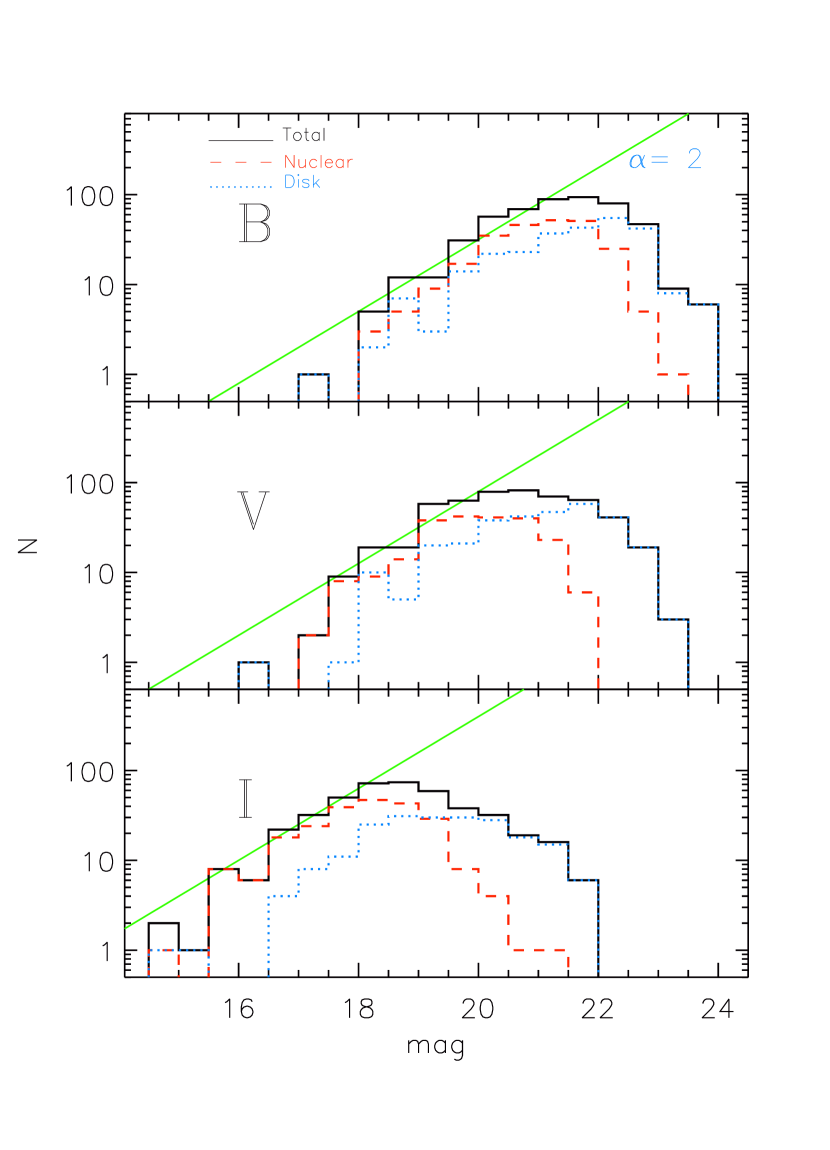
Figure 2.— Magnitude histogram of detected clusters in the $B,V$ and $I$-bands. Separate histograms are drawn for the nuclear and disk clusters. The solid line corresponds to a power-law of index of 2.0 in the luminosity function.

In Figure 2, we show the luminosity function of sources satisfying our selection criteria of clusters for each of the $B,V$ and $I$ images, independently. The luminosity functions in every band show an apparent turn-over with the distributions being consistent with a power-law form of index $\alpha=2$ on the brighter side, and falling steeply on the fainter side. Selection criterion 1 is responsible for the steep fall as discussed in §2.1. The turn-over magnitudes are equal to $\sim$21.5, 20.5, and 18.5 in the $B,V$ and $I$-bands, respectively. At the very bright end of the luminosity function, when the numbers expected from the extrapolation of the power-law are below 10, the observed numbers are systematically lower in all the bands. It seems that we are missing around 5 bright clusters. This may suggest the existence of an upper limit to the cluster masses as advocated by Gieles et al. (2006a). On the other hand, it is also possible that the under-abundance of bright clusters is due to the combined effects of high extinction, and small number statistics. The nuclear and disk cluster samples present similar luminosity functions, with the apparent turn-over magnitude $\sim 0.5$ mag fainter for the latter sample.

2.3. Cluster size distribution

SExtractor provides the FWHM of a fitted Gaussian profile for each source. We have adopted this figure of merit as a measure of the size of the clusters, instead of the often used half-light radius ($R_{\rm eff}$). This is because the Gaussian FWHM is uniquely defined for a source, and can be measured with the same accuracy for bright and faint regions, whereas the value of $R_{\rm eff}$ is very sensitive on the parameters of the fitted analytical function (Larsen, 2004). SExtractor calculates the half-light radius, that we found is related to the FWHM (both in pixel units) by the equation: $R_{\rm eff}=1.0+0.33\times{\rm FWHM}$. The values of $R_{\rm eff}$ calculated from this relation may differ slightly from those values determined based on an analytical function. We use this equation only for the purpose of comparing the mean FWHM obtained in this work with $R_{\rm eff}$ quoted in the literature for other galaxies.

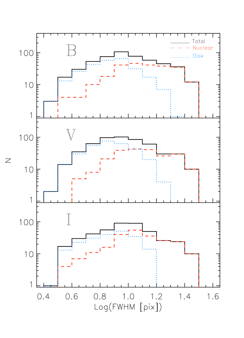
Figure 3.— The observed cluster size distributions are plotted for the $B,V$ and $I$ photometric bands for the entire, the nuclear, and disk cluster samples considered in this work. In every case, we see that the size distribution function is log-normal with a peak at about 10 pixels.

The histograms of Gaussian FWHMs in the $BVI$ photometric bands, for the total, nuclear and disk samples, are presented in Figure 3. There, it is evident that the observed CSF peaks at a characteristic value of about 10 pixels FWHM or $R_{\rm eff}=3.8$ pc. Melo et al. (2005) found a mean radius value $5.7\pm 1.4$ pc for the M82 nuclear clusters. However, their values cannot be directly compared with ours as they had defined the radius as the inflexion point of the photometric growth curve in $B$ and H$\alpha$ bands. On the other hand, our values are in good agreement with those measured in a sample of 18 nearby spiral galaxies, where Larsen (2004) reported a mean value of $R_{\rm eff}=3.94\pm 0.12$ pc. The presence of a characteristic cluster size is quite different to what was found in M51, where the size distribution follows a power-law function (Bastian et al., 2005; Scheepmaker et al., 2007).

3. Monte Carlo simulations

The observed cluster luminosity function follows a power-law at the bright end, turning over sharply at faint magnitudes. Similarly, the CSF peaks at a characteristic value of $\sim$10 pixels FWHM. In order to investigate whether observational biases are responsible for these turn-overs, we carried out detailed Monte Carlo simulations.

We have used simulations in order to generate a $B$-band ACS image of M82 containing N_sim clusters. The luminosity function of the simulated clusters is defined by a power-law distribution in the 18–25 magnitude range: $dN/dL\propto L^{-\alpha}$. A power-law index $\alpha=2$ was adopted, that corresponds to a slope of 0.4 in the $\log(dN/dmag)$ versus magnitude plot. In the simulations, each cluster is assumed to be round and to have a Gaussian intensity profile of a given FWHM. We used two functional forms for the size distribution of the clusters: the first one adopting a power-law function ($dN/dS\propto S^{-\beta}$) with an index $\beta=3.3$. In the second simulation, we adopted a log-normal function peaking at 10 pixels with a $\sigma$ value of 2 pixels. We generated N${}_{\rm sim}=11855$ clusters, the number of extended objects in the observed $B$-band source list with an area of at least 35 pixels. The location of the observed sources were used as their reference positions of the simulated clusters. This procedure simulates properly the crowding of sources observed in M82. We also generated point sources as Gaussian profiles of FWHM fixed at 2.1 pixels, with their positions and magnitudes corresponding to the observed values. The precise position of every source (stars and clusters) is generated by randomly placing them within an rms of 10 pixels around that in the source list.

In order to emulate as closely as possible the observed conditions, we degraded the noise-free simulated image by adding the observed rms noise ($\sigma_{B}=0.006$ count/pixel/sec), and the SExtractor-generated background image of M82. The SExtractor was run on the simulated image with the same set of parameters that were adopted for the observed $B$-band image. The resulting catalog was passed through the same selection filters described in § 2.1 in order to obtain a catalog of simulated clusters.

Figure 4.— Differences (recovered$-$original) between the recovered B-band magnitudes and FWHMs of individual clusters compared to their simulated values, plotted against the simulated magnitude (top) and FWHM (bottom). The histograms of the differences are shown for all the recovered sources in the top panel. In the bottom panel, the histograms are shown separately for the compact (dashed line) and loose (solid line) clusters, with FWHM=10 pixels, being the dividing value. The results shown here are for a log-normal size distribution, but are very similar for the power-law size distribution.

We compared the extracted $isocor$ magnitude and FWHM size of every cluster with the simulated values. Results are summarized in Figure 4. The histograms of the differences have a maximum at $\Delta=0$, indicating that SExtractor accurately recovers magnitudes and sizes of the simulated sources. For 90% of the recovered sources, magnitude difference is less than 0.1 mag, while FWHM size difference lie within 0.75 pixel of the simulated values. For the remaining 10% of the sources, the extracted magnitudes and sizes turn out to be systematically brighter and larger. Both effects are consequence of the superpositions of more than one simulated source due to crowding that extractor code identifies as a single source. Photometric recovery is better than 0.1 magnitude for both extended and compact sources, which illustrates that there is no systematic underestimation of flux, as measured by $isocor$, from extended sources.

3.1. Simulated Luminosity Function

Figure 5.— Histogram of SExtractor recovered B-band magnitudes of simulated clusters are shown separately for the nuclear (dotted line) and disk (solid line) of M82. The simulated power-law function of index=2 is shown. Recovered sources follow the power-law function up to $\sim 21.5$ mag, beyond which the fraction of recovered sources decreases, reaching zero at 25 magnitude. Hence, the observed turn-over at $B\sim 21.5$ mag is an artifact of incompleteness and not a physical turnover.

The luminosity function of the simulated clusters is plotted in Figure 5, separate histograms are shown for the nuclear and disk samples. At the bright end, luminosity functions of the recovered sources follow the same power-law that was used to generate them. The distribution function for the extracted disk clusters begins to depart from the simulated one at $B\sim 21.5$ magnitude, remains nearly flat for another 2 magnitudes before falling sharply at fainter luminosities. The fraction of the simulated sources recovered is larger than 90% for sources brighter than 21.0 mag, falling to $\sim 60$% at 22 magnitude, which we refer to as the apparent turn-over magnitude. The luminosity distribution function for the nuclear clusters is very similar to that for the disk population except that the apparent turn-over magnitude is $\sim 0.5$ mag brighter than that for the disk. The higher nuclear background, and greater crowding as compared to those of the disk are responsible for the difference.

The simulated luminosity function resembles very much the observed one, implying that the observed apparent turn-over of the luminosity function is due to incompleteness at the faint end and not intrinsic to the cluster population. Hence, the intrinsic turn-over in the luminosity function, if any, would correspond to a magnitude fainter than $B=22$ mag. We find that the power-law index ($\alpha=2.0$) can be recovered to within an error of 0.1 using only the data brighter than the apparent turn-over magnitude, independently for the nuclear and disk clusters. This ensures that reliable value of $\alpha$ can be determined from the observed data.

3.2. Simulated Size Function

Having established that the turn-over in the luminosity function is caused by the incompleteness in the detection of faint clusters, we now investigate whether the CSF is also affected by our selection criteria. From simple analytical calculation of the type presented in Table 1, we find that the clusters that survive our first selection criterion all the way to $B=24$ mag are those with intermediate sizes (FWHM$\sim$5–11 pixels), with the rest of the clusters having cut-off magnitudes between 22–24. The rejection of clusters is mainly because they fail to satisfy the requirement of at least 50 pixels area. Thus, the CSF derived from a sample that includes clusters fainter than the apparent turn-over ($B=22$ mag) is not expected to represent the true distribution. We used the results of Monte Carlo simulations to check whether the CSF obtained using clusters on the brighter side of the apparent turn-over represents the true distribution.

Figure 6.— Histograms of the distribution of FWHM of the simulated clusters are shown for a log-normal (top) and a power-law ($\beta=3.3$, bottom) function. Separate histograms are drawn for the clusters recovered by the SExtractor in environments appropriately matching those of the nuclear and disk of M82. For both the simulated functional forms, the recovered distribution maintains its original form.

We plot the size distribution function for the simulated data in Figure 6. Only clusters brighter than $B=22$ mag in the disk, and $B=21.5$ mag in the nucleus, were used in creating these histograms. Separate histograms are shown for the nuclear and disk clusters. The top and bottom panels show the histograms for a log-normal and power-law types of distribution functions, respectively. The recovery of the simulated size distribution functions is very good for both types of functional forms for FWHM$\lesssim 15$ pixels. In particular, a power-law distribution retains its form and index value both for the disk and nuclear samples. Thus, the observed log-normal distribution of sizes couldn’t have been the result of selection effects transforming an intrinsically power-law into a log-normal distribution. Clusters with FWHM$>15$ pixels are not detected even at magnitudes brighter than the apparent turn-over. This explains the absence of such clusters in the observational data (Figure 3).

From the analysis of the simulated luminosity function we have inferred that around 10% of clusters brighter than $B=21$ mag, and 40% of clusters brighter than $B=22$ mag are not detected. Analysis of simulated data presented in Figure 6 offers us an opportunity to understand the reasons for the non-detection. One of the reasons is that they are too extended (FWHM$>15$ pixels). Among the rest, the cluster detection fraction doesn’t dependent on the value of the FWHM. Rather, the reason for the non-detection is that either the cluster is situated in a region with higher than average background value or that there is a bright cluster in its vicinity. Thus, our simulations illustrate that there is no size-dependent bias against the cluster detection as long as they are brighter than $B=22$ mag and have FWHM$<15$ pixels. Hence, the size function derived using data of clusters brighter than the apparent turn-over is a true representation of the intrinsic function.

4. Physical Parameters of Clusters

M82 is a spiral galaxy seen almost edge-on (Mayya et al., 2005), consequently the effect of obscuration is severe. Hence, the physical parameters derived from observational data critically depend on the treatment of the interstellar extinction. The issue of extinction toward the nuclear starburst of this galaxy has long been the subject of study. Rieke et al. (1993), using near infrared recombination lines integrated over the central starburst region, estimated visual extinction values between 12 and 27 magnitudes, the exact value depending on the adopted reddening model. Förster Schreiber et al. (2001) found $A_{v}\sim 10$ mag in selected knots using a uniform foreground screen model, and $A_{v}>23$ mag for models where dust and stars are mixed. In this section, we analyze the observed colors and brightness of the clusters with the aim of deriving extinction corrected photometry, and compare them with a population synthesis model.

4.1. Population Synthesis Models

Star clusters can be considered as simple stellar populations (SSPs), and some of their physical parameters such as mass and age can be obtained from the analysis of their colors and luminosity with the help of population synthesis models. In this work, we have used the solar metallicity SSP models of Girardi et al. (2002). These authors had carried out the evolution of colors and magnitudes for the instrumental HST/ACS filters, a fact that enables us a direct comparison with the observed data. The Kroupa (2001) initial mass function (IMF) in its corrected version has been used. It has nearly a Salpeter slope (2.30 instead of 2.35) for all masses higher than 1 $M\odot$. The derived masses depend on the assumption of the lower cut-off mass of the IMF. In the case of standard Kroupa’s IMF, the derived masses would be around 2.5 times higher.

4.2. Analysis of Colors

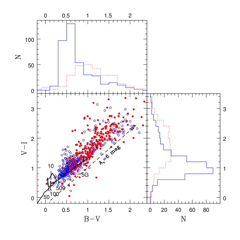
Figure 7.— Nuclear (solid circles) and disk (open circles) clusters in $V-I$ vs $B-V$ plane. Evolutionary track for an SSP is shown by the solid line, with the tick marks denoting the location at ages of 10, 50, 100, 500 Myr and 5 Gyr. The reddening vector corresponding to $A_{v}=6$ mag is shown. The histograms of each axis are shown, separately for the disk (solid line) and nuclear clusters.

The observed cluster colors are plotted in the $V-I$ vs $B-V$ plane in Figure 7. The filled circles correspond to the nuclear clusters, whereas open ones correspond to the disk clusters. The solid line represents the locus of an SSP evolutionary track. Time tags represented by vertical lines correspond to SSP ages 10, 50, 100, 500 Myr and 5 Gyr. There, a reddening vector corresponding to $A_{v}=6$ mag is also shown. The histograms corresponding to the distribution of the colors are shown in the top and right side panels, separately for the disk (solid line) and the nuclear clusters. It can be seen that the distribution of colors of disk clusters peaks at lower values and has a smaller spread as compared to those of the nuclear clusters. The color distributions have a long red tail for both classes of clusters. The red tail of the distribution reaches colors even greater than those of a 5–10 Gyr old population. Thus, the large observed color range is produced by a large spread in the reddening rather than a spread in the age. Hence, the observed colors are useful in deriving the amount of reddening, given a value for the cluster age.

4.3. The ages of clusters

The stellar population in the nuclear region of M82 has been the subject of innumerable studies. Rieke et al. (1993) found that the multi-wavelength data for the central 400 pc region of M82 can be explained by a few starburst events over the last 30 Myr. More recent study by Förster Schreiber et al. (2003) favors the presence of two short-term bursts over the last 10 Myr. Satyapal et al. (1997) studied 12 nuclear star clusters of M82, and found their ages to be between 4–10 Myr. Melo et al. (2005) found that a great majority of the nuclear star clusters are associated with H$\alpha$  emission, suggesting that they are younger than the lifetime of ionizing O stars. Based on these results, we adopt an age of 8 Myr for the nuclear clusters.

The H$\alpha$  emitting regions are exclusively located in the central starburst region, and in the cone along the minor axis of M82. The absence of H$\alpha$  emission in the disk implies that currently there is no significant amount of star formation. The disk is known to be rich in the Balmer absorption lines, suggesting an intense star formation in the past (O’Connell & Mangano, 1978). Mayya et al. (2006) made use of these spectral features to infer a rather young age for the disk in M82. The disk stars were formed in a burst as a consequence of a tidal interaction with members of M81 group during the last 500 Myr. Were the clusters formed simultaneously with the disk-wide star formation? To answer this question, spectroscopically derived ages of clusters would be required. Such data are available only for four disk clusters — regions F and L, and two clusters in the region B (Smith et al., 2006). Derived ages range between 50–65 Myr for F and L, and $\sim 350$ Myr for the two optically bright knots in region $B$. We have used the ACS photometric data to check whether the ages of these bright clusters are representative of that of the bulk of the population. As discussed previously, the colors in M82 are strongly affected by reddening, and hence any age inference based on colors of individual clusters is not expected to give a unique solution. We investigated whether the color differences between the clusters and the surrounding disk could be used to derive a statistical age for the cluster population in the disk. If the clusters have a similar age as that of the stellar disk, and if the reddening is caused by the dust clouds external to the clusters, then the color distribution of the clusters would be similar to those of the local disk. We carried out experiments to test this idea.

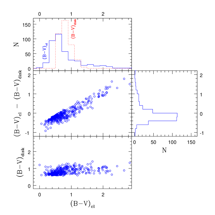
Figure 8.— Distribution of the $B-V$ colors of clusters compared to that of the surrounding local disk. (bottom panel) Color of the local disk surrounding a cluster is plotted against the color of the cluster. (middle left panel) Difference of the colors of disk clusters with respect to that of the surrounding disk plotted against the cluster colors. The histograms of each axis are shown. The majority of the clusters (85%) are bluer than the surrounding disk, suggesting that clusters in general are younger than the disk. However, the red colors of the remaining clusters are correlated with its “excess” from the disk, implying that they are heavily reddened.

We measured the colors of the disk surrounding every cluster in a 10-pixel wide annulus with an inner radii of 20, 30 and 40 pixels, that correspond to 1, 1.5, and 2^′′, respectively. We found that the colors in these three annuli are very similar. In Figure 8, we compare the colors of the inner most annulus with that of the corresponding cluster. In the bottom panel, the disk $B-V$ color is plotted against that of the cluster. There, we can see that the disk colors span a much shorter range as compared with that of the clusters. In fact, the color difference (middle panel) of the cluster and the local disk reflects the color of the cluster. The peak of the cluster color distribution is at $\sim 0.2$ mag bluer than the surrounding disk. Systematically blue colors of the clusters suggest that the clusters are younger than the disk. Interestingly enough, the disk surrounding the red clusters is not as red, suggesting that the dust causing the reddening of the clusters is local to the cluster, perhaps associated with the interstellar medium left over from the star formation episode. Very similar results are found from the analysis of the $V-I$ colors.

The bluer colors of the clusters could be due to metallicity effects, if the clusters have systematically lower metallicity content as compared to the local disk. This case is unlikely, yet it could happen if the clusters were formed from the accreted metal-poor gas, after the formation of the disk. In this scenario, clusters would be at the most as old as the disk. On the other hand, if the cluster stars are of higher metal abundance, they could be as young as 50 Myr. This rather young age compares very well with the 50–65 Myr determined by Smith et al. (2006) for the bright clusters $F$ and $L$ from spectroscopic indices. Consequently, the ages of the disk clusters are most likely lie in the 50–500 Myr range. For the determination of reddening and mass of individual clusters, we fix their age at 100 Myr, and discuss the error on these quantities if they were as young as 50 Myr or as old as 500 Myr.

4.4. Color-Magnitude Diagrams

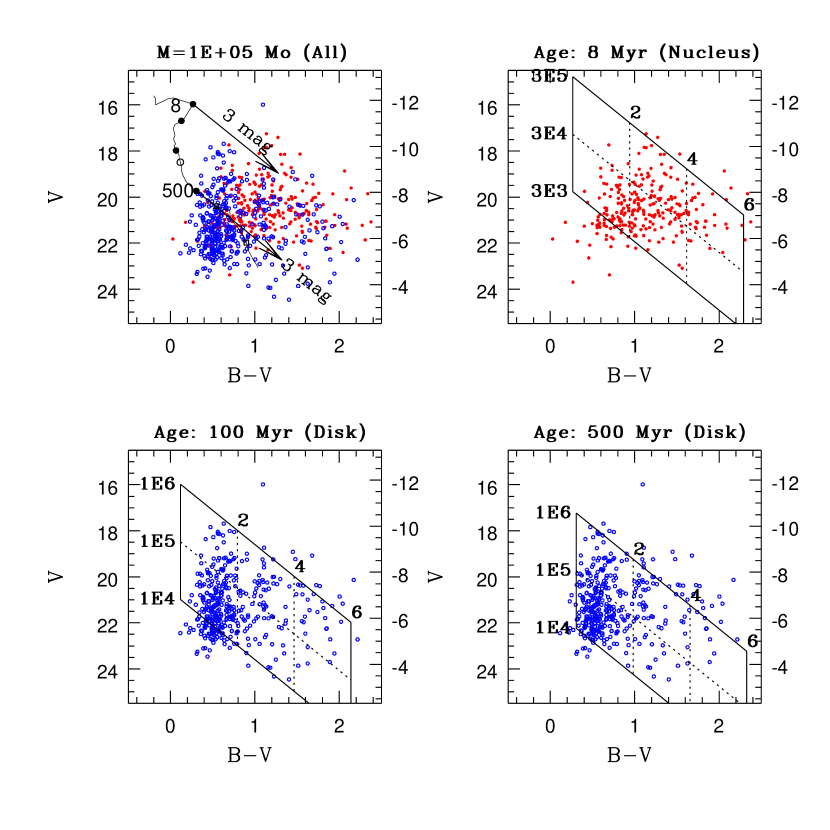
Figure 9.— Observed color-magnitude diagrams (CMDs) for the nuclear (filled circles) and disk clusters, in M82. (Top left) Evolutionary track for an SSP of a cluster mass of $10^{5}$ $M\odot$ is superposed. Two vectors, placed at 8 Myr and 500 Myr, show the location of the track reddened by $A_{v}=3$ mag. In the top-right panel, we show the CMD for the nuclear clusters only. The locations of an 8 Myr SSP for a range of cluster masses and visual extinctions are shown by the superposed grid. Mass varies vertically along the grid (in solar units), whereas the visual extinction (in magnitude) varies along the diagonal axis. In the bottom panels, we show a similar diagram for the disk clusters, with the superposed grids corresponding to fixed ages of 100 Myr (left) and 500 Myr (right). In all the panels, tick mark values of the right-vertical axis correspond to the absolute magnitude. In the derivation of mass and visual extinction values, we adopt a uniform age of 8 Myr for the nuclear, and 100 Myr for the disk clusters.

Once the reddening is derived using the colors, we obtain masses of individual clusters with the help of the SSP for the assumed age (8 Myr for the nuclear clusters, and 100 Myr for the disk clusters). The method we have followed is illustrated in Figure 9. For a given position in the Color Magnitude Diagram (CMD), we derived the reddening by comparing the observed colors with those of the SSP. Cardelli et al. (1989) extinction curve with Rv=3.1 is used to convert reddening to visual extinction $A_{v}$. The mass is then calculated using the extinction-corrected $B$-band luminosity and the mass-to-light ratio of the SSP for the assumed age.

In Table 3, we list the derived quantities (visual extinction, extinction corrected B-band absolute magnitude and mass) along with their estimated errors for every cluster. We have independently derived extinction values from $B-V$ and $V-I$ colors, and the tabulated values are the mean of the two measurements. The dispersion from the mean value is tabulated as the error on $A_{v}$. The absolute $B$ magnitude listed is extinction-corrected. The tabulated mass is photometric and is obtained by the method described above, using an age of 8 Myr for the nuclear clusters, and 100 Myr for the disk clusters. The derived $A_{v}$ would be systematically higher by 0.12 mag if the disk clusters are as young as 50 Myr, and lower by 0.58 mag if they are as old as 500 Myr for the SSPs used in this work (Girardi et al., 2002). The derived disk masses would also be different if we had used a different age, as both the extinction and mass-light-ratio are sensitive to the assumed age of the population. Fortunately, these two corrections act in opposite directions, with the net result that the masses would always be within a factor of 1.5 of the tabulated values for the range of ages between 50–500 Myr. The errors on $B$ magnitude and masses are calculated by quadratically summing the errors on $A_{v}$ and the $B$ magnitude, the latter taken as 0.2 mag for all clusters.

Figure 10.— Histogram of visual extinction ($A_{v}$) for the nuclear and disk clusters. Nuclear clusters experience a higher extinction as compared to the disk clusters.

The histogram showing the distribution of visual extinction for an assumed age of 8 Myr for the nuclear, and 100 Myr for the disk clusters, is plotted in Figure 10. The distribution for the nuclear clusters is nearly flat between $A_{v}=$1.0–4.0 mag, whereas it is peaked at $\sim 1$ mag for the disk clusters. There are a few clusters in both the disk and the nucleus with inferred $A_{v}>$6 mag. The derived $A_{v}$ is less than 2.0 mag for 85% of the disk clusters, whereas only 20% of the nuclear clusters are below this value. The results remain practically the same if all the disk clusters are as young as 50 Myr. On the other hand, if all the disk clusters are as old as 500 Myr, the distribution of their $A_{v}$ would peak at a value lower by 0.58 mag ($\approx 1$ bin width) with respect to that in Figure 10. This would further increase the mean difference in the extinction values between the disk and nuclear clusters.

4.5. Cluster Mass Distribution Function

Figure 11.— Mass functions for the nuclear (dotted line) and disk (solid line) cluster samples. Both the samples follow a power-law distribution between $2\times 10^{4}$$M\odot$ and $10^{6}$$M\odot$. The best-fit indices in this mass range are indicated.

The derivation of the cluster masses for our entire sample enables us to derive the present-day CMF. In Figure 11, we plot the CMF separately for the nuclear and disk clusters. The nuclear CMF is scaled up to match the disk CMF at $1.5\times 10^{6}$ $M\odot$. Poissonian error bars are indicated. The distribution for both samples follows a power-law over almost two orders of magnitude in mass for cluster masses above $\sim 2\times 10^{4}$ $M\odot$. However, the power-law index for the disk and nuclear cluster populations shows a marginal difference, $\alpha=1.8\pm 0.1$ for the nuclear clusters, and $\sim 1.5\pm 0.1$ for the disk population. A different choice of age (within the range 4–10 Myr for nuclear clusters and 50–500 Myr for the disk clusters) in the derivation of the photometric mass would have only changed the masses by less than the size of the bin width used in Figure 11. Hence, the slopes of the mass functions are not affected by our assumption that all the clusters in each zone have the same age.

Studies of young star clusters in nearby galaxies yield a value for $\alpha$ close to 2.0 (de Grijs et al., 2003c). Our derived value of $\alpha=1.8\pm 0.1$ for the M82 nuclear clusters is marginally flatter than this. On the other hand, the mass function of the disk clusters is clearly flatter than that for young clusters, implying that the low-mass clusters are selectively lost as the cluster population evolves. In order to shed more light on the missing population, we analyze the cluster size distribution below.

4.6. Cluster Size Distribution Function

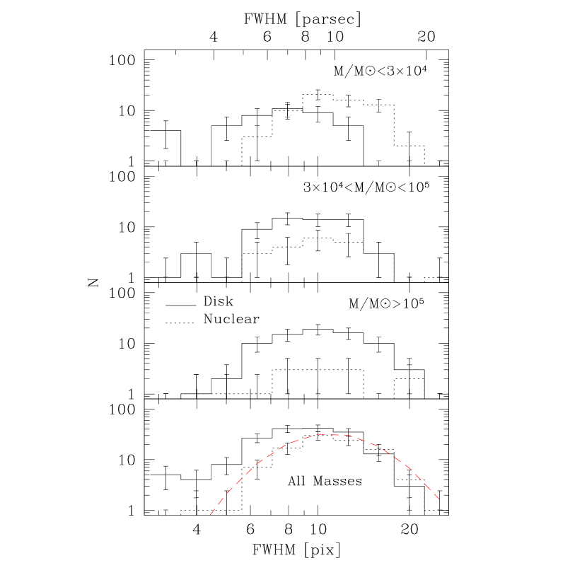
Figure 12.— Size function for all the detected clusters (bottom panel). In the top three panels, the size function is shown for three different mass bins. In each panel, histograms are drawn separately for the nuclear and disk clusters. A log-normal distribution function is drawn fitting the nuclear cluster sample (dashed line) in the bottom panel.

In Figure 12, we compare the CSF for the nuclear and disk samples. Following the discussion in §3.2, only clusters brighter than the apparent turn-over luminosity ($B=22$ mag for the disk and $B=21.5$ mag for the nucleus) were considered. The mass that corresponds to the apparent turn-over is $\sim 2\times 10^{4}$$M\odot$, and hence the plotted functions are representative of the cluster population more massive than this limit. The CSF for the nuclear region can be fitted very well with a log-normal function centered at FWHM of 11 pixels ($\sim 10$ pc). On the other hand, the CSF for the disk clusters is quasi log-normal: a log-normal fit to the distribution of clusters with sizes larger than 11 pixels underestimates the actual number of observed compact clusters, while a fit to the distribution of compact clusters shows a deficiency of extended or loose clusters. In order to investigate the possible origin of the skewness in the distribution, we have analyzed the size distribution function in three separate mass bins, i.e. low-mass (mass$<3\times 10^{4}$$M\odot$), high-mass (mass$>10^{5}$$M\odot$) and intermediate mass (all in between). The CSF for the nuclear clusters follows the log-normal distribution in each of the three mass bins (taking into account the statistical errors caused by the small number of clusters in the highest mass bin). The disk clusters in the highest mass bin, also follow a log-normal distribution. The CSF of the lower mass clusters of the disk, however, depart from that of the nuclear clusters: the largest clusters, as well as the mean cluster size, are systematically smaller for the lower mass bins. This tendency is illustrated in Figure 13, where the mean cluster size for each mass bin has been plotted against the mean mass of clusters in that bin, for the young and old ones, separately. For the highest mass bin, the mean sizes of the young and old clusters are similar. The mean size decreases systematically with decreasing cluster mass for the old clusters, whereas the inverse is true for the young clusters.

Figure 13.— Mean size (FWHM) of the clusters as a function of mean mass for three mass bins for the nuclear (young) and disk (old) samples. The error bar denotes the rms dispersion about the mean value. High mass clusters have similar mean sizes irrespective of their evolutionary status. On the other hand, mean size of the low-mass clusters decreases as they become older. Among the young clusters, low-mass ones are more extended than higher mass ones.

Systems in Virial equilibrium are expected to follow a power-law radius-mass relation ($R\propto M^{\gamma}$) with a $\gamma=0.5$, the most common examples being the Giant Molecular Clouds (GMCs) and elliptical galaxies. Stars of a cluster are well mixed and reach Virial equilibrium after just a few crossing times (King, 1981). M82 clusters are around ten crossing times old and hence are expected to be in Virial equilibrium (McCrady & Graham, 2007). The relationship seen in Figure 13 corresponds to a power-law index of $\gamma=0.05$, and $-0.02$, for the old and young samples, respectively, i.e. both values are significantly flatter as compared to those of bound systems in Virial equilibrium. On the other hand, our values for the disk clusters are in excellent agreement with that found ($\gamma=0.08\pm 0.03$) for star clusters in nearby galaxies by Larsen (2004). McCrady & Graham (2007) have obtained an index of $\gamma=-1$ for clusters losing mass adiabatically over time. Thus, mass-loss from clusters could yield a flatter radius-mass relationship. The similar observed range of sizes for high-mass clusters independent of whether they are young or old suggests that these clusters have reached their equilibrium sizes and that the evolution hasn’t played a role in changing their sizes. The observed radius-mass relationship then implies that the sizes of lower mass clusters are well above their equilibrium values, or in other words they are distended ones. On an average, younger clusters are farther from equilibrium values as compared to older ones. Together, these results imply that many of the young low-mass clusters in our sample are loosely bound or unbound, or probably are expanding OB stellar associations. The extended low-mass clusters are being selectively destroyed as a function of time, whereas compact clusters of all masses have survived. However, the sizes of even the most compact low-mass (mass$\lesssim 5\times 10^{4}$ $M\odot$) clusters are larger than their Virial expected values, implying that they are expanding and may not survive over the Hubble time.

The observed differences in the CSF for young and older clusters are consistent with the expected evolutionary effects. Both, the disruption of the loose OB associations and the dynamical trend towards relaxation would diminish the number of large low-mass systems. Thus, the destruction process is both mass and size dependent, with the most extended clusters in each mass bin being the first ones to be dispersed. The near equality of the mean size for young and old clusters of masses higher than $\sim 10^{5}$ $M\odot$ implies that all high mass clusters survive for ages more than $\sim 10^{8}$ yr or that the destruction process is independent of the size for these high mass clusters. In the next section, we will discuss these observational results in the context of results obtained by other studies, and propose the most likely scenario of cluster disruption in M82.

5. Discussions and conclusions

The presence of two populations of star clusters in M82, one young (age$<10^{7}$ yr), and the other relatively old (age$\sim 10^{8}$ yr) allows us to interpret the observed differences of their distribution functions in terms of evolutionary effects. We start this section by comparing our CMF for the entire disk, with that published for the region B in M82.

5.1. M82 B and the Initial Cluster Mass Function

The bright blue region known as M82 B about a kiloparsec distance to the northeast of the nucleus has been the subject of study in a series of articles (de Grijs, O’Connell & Gallagher, 2001; de Grijs et al., 2003a, b). These authors were able to detect more than 200 cluster candidates using the HST/WFPC2 images, which were used to construct luminosity and mass functions. They found that the mass function is log-normal with a turn-over in the mass function at $\log$(mass)$=5.1\pm 0.1$, well above their completeness limit for cluster detection. Adopting an estimated age of 1 Gyr for this system, they argued that the log-normal mass distribution cannot be the result of selective destruction of smaller clusters as the clusters evolve, and instead should have been born that way. In essence, they favored a log-normal initial CMF for M82 clusters, and proposed that the GCs probably were also born with log-normal initial CMF.

A log-normal initial CMF is not consistent with our dataset for younger clusters in M82. In fact, both the younger and older clusters of our sample follow power-law forms, with the index being marginally different for the two populations. More importantly, the apparent turn-over masses for the two samples are similar, and are at least a factor of five lower than that reported by de Grijs et al. (2003a). Bright clusters of M82 B make part of our sample, and hence these differences are intriguing.

The explanation for the different conclusions lies in the different adopted ages: 100 Myr (ours) versus 1 Gyr (de Grijs et al., 2003a). Available spectroscopic data favor ages between 50–350 Myr: Smith et al. (2006) derived an age of $\sim 350$ Myr for two knots (B2-1 and B1-1) in region M82 B, and 50–65 Myr for the knots F and L at similar galactocentric distance as region B, but to the southwest of the nucleus. Recent determination of ages for 7 more clusters by Konstantopoulos et al. (2007) also support these relatively younger ages. Thus, an age of 1 Gyr seems extremely high for the cluster population in M82, and the ages are likely to be closer to the one we have adopted. The $B$-band luminosity drops by a factor of 8.5 due to passive evolution of SSPs between 100 Myr and 1 Gyr (Girardi et al., 2002). Thus, the photometrically derived masses by de Grijs et al. (2003b) could have been overestimated by a factor as large as this. If we take into account this factor, their turn-over mass values would be similar to the ones we find in the present study. A lower turn-over mass dilutes the case for a log-normal initial CMF.

5.2. Disruption of clusters: mass and size dependence

Whether low-mass clusters are preferentially disrupted with respect to the high mass ones is the question waiting to be answered by the ever growing data on extragalactic star clusters. So far, the best studied cases are M51 and the Large Magellanic Cloud (LMC). For M51 clusters, Bastian et al. (2005) concluded that the disruption rate at early times ($\sim 10$–30 Myr) is independent of cluster mass. In the LMC, de Grijs & Parmentier (2007) report evidence for mass-dependent disruption for masses below a few $\times 10^{3}$ $M\odot$. Our result showing a tendency for a flatter slope of the mass function at older ages is an indication that the disruption processes acting in the disk of M82 are mass-dependent.

For a given mass, clusters of larger radii are loosely bound, and it is easier to disrupt them. Hence, one would expect those clusters to be missing in older cluster samples. Gieles et al. (2005) found size-dependent evolution for the M51 clusters. In the Antennae galaxy, Mengel et al. (2005) have found a decrease of the average cluster size with age, as well. In the present study, we find that the average size of the clusters is smaller for older clusters of mass $<10^{5}$ $M\odot$. Thus, evolutionary processes selectively disrupt loosely bound clusters.

5.3. Physical processes driving the disruption

In the introduction, we have mentioned several physical processes that are capable of disrupting a star cluster. We refer the readers to the works of Spitzer (1987), Fall & Zhang (2001) and de Grijs & Parmentier (2007), for details on these physical processes. At early times ($t\lesssim 30$ Myr), disruption is caused mainly due to the expulsion of the intra-cluster gas through supernova explosions. This process is independent of cluster mass, as long as the stellar IMF, or the mass fraction of the gas, are not systematically different for low and high mass clusters. The other process that can change the slope of the cluster mass function is the tidal shock experienced by the clusters as they move in the gravitational field of a galaxy. According to Fall & Zhang (2001), this process becomes important after $\sim 300$ Myr in normal galaxies. However, in the case of M82, de Grijs et al. (2005) have estimated a disruption timescale as short as 30 Myr for a cluster of mass $10^{4}$ $M\odot$  at 1 kpc away from the center, with a dependence on mass that varies as $M^{0.6}$. Hence, the derived slope of $\alpha=1.8$ for the nuclear clusters, which are younger than 10 Myr, likely represents the initial slope of the mass function. On the other hand, clusters in the disk of M82 are expected to suffer from the dynamical processes of cluster disruption. This kind of disruption process destroys first the larger clusters. The over-abundance of compact clusters in our sample of the older clusters, as compared to the sample of younger clusters, is quite consistent with this idea. Thus our dataset support the relatively short disruption timescale estimated for M82.

5.4. Initial size distribution function

Very little is known regarding the distribution of sizes of SSCs. For clusters in M51, Bastian et al. (2005) found a power-law relationship with an index of $2.2\pm 0.2$, which agrees well with that for the galactic globular clusters ($2.4\pm 0.5$). Using more recent HST/ACS data of M51, Scheepmaker et al. (2007) also find a power-law form for the CSF, albeit over a much smaller range in sizes. In the case of M82, the power-law form is not evident in the observed distribution of sizes of bright clusters considered in the present study (Figure 12): we should have detected large numbers of compact clusters, which is not the case. As compared to our sample in M82, the low-mass limit in the cluster samples of M51 (Bastian et al., 2005; Scheepmaker et al., 2007) is an order of magnitude lower. If the low-mass clusters are systematically more compact than their high-mass counterparts, then the observed difference in the functional forms of the two galaxies can be understood in terms of the difference in the low-mass limits. However, no clear mass-radius relation was found for M51 clusters. Hence, the CSF for the bright cluster in M82 is different from that found in M51.

It is likely that this difference might be related to the relative youth of the disk of M82. In a galaxy with clusters forming continuously over time, the selective disruption of large clusters is expected to induce an accumulation of clusters of the smaller sizes at any given cluster mass. This cumulative process seems to have taken place in M51, while in M82 we are likely witnessing the initial distribution of sizes.

6. Summary

In this study, we have carried out an objective search for star clusters on the HST/ACS images of M82 in filters F435W(B), F555W(V), and F814W(I). The search has led to the discovery of 393 clusters in the disk and 260 clusters in the nuclear region. The magnitude and FWHM of these clusters were used to construct luminosity and size distribution functions. We find that the luminosity function follows a power-law with an index of 2, with an apparent turn-over at the faint end. Monte Carlo simulations carried out by us show that this turn-over is a consequence of incompleteness in the detection of faint clusters rather than a turn-over in the intrinsic luminosity of the population. We used simple stellar population synthesis models to derive visual extinction values and photometric masses for the clusters, adopting a uniform age of 8 Myr for the nuclear clusters and 100 Myr for the disk ones. The resultant mass distribution functions for the nuclear and disk regions follow power-law functions, with a marginally steeper index value of 1.8 for the younger nuclear regions as compared to 1.5 for the older disk regions. The cluster size distribution function, constructed for the clusters brighter than the turn-over magnitude, follows a log-normal function with its center at 10 pc FWHM ($R_{\rm eff}\sim 4$ pc) for the most massive clusters (mass $>10^{5}$ $M\odot$). For lower masses (mass=(0.2–1.0)$\times 10^{5}$ $M\odot$), the center is marginally shifted to larger values for the younger, and smaller values for the older clusters. This tendency implies that the extended low-mass clusters are selectively destroyed during their dynamical evolution. The marginally flatter slope of the mass function, and an over-abundance of compact clusters in the older sample, are pointing towards a mass and size dependent cluster disruption process at work in the disk of M82.

Table 1Exposure times and limiting magnitudes for stars and clusters .

Filter	Exp Time	m(star)	m(cluster)
	seconds		compact	extended
F435W (B)	1600	25.67	21.76	23.97
F555W (V)	1360	25.18	21.27	23.48
F814W (I)	1360	24.24	20.32	22.53

Table 2Source detection statistics in M82

Source type	$B$	$V$	$I$	Selection Criteria
All	44274	82515	151565	5–10 $\sigma$/pixel
Extended	83%	77%	60%	$3\leq FWHM/{\rm pix}<30$
Candidates	7632	7688	6307	$3\leq FWHM/{\rm pix}<30$ & $area>50$ pix
Clusters	421 (263)	456 (306)	390 (208)	see $\S$2.1

Table 3Photometric properties of detected star clusters in M82

ID	$B$	$\sigma(B)$	$B-V$	$V-I$	$A_{\rm v}$	$\sigma(A_{\rm v})$	$M_{B}^{0}$	$\sigma(M_{B}^{0})$	$\log(M\ast)$	$\sigma(\log({\rm M\ast}))$	Other ID
1N	18.39	0.01	1.14	1.57	2.38	0.00	$-12.63$	0.20	5.42	0.08	H
2N	18.43	0.01	0.69	0.93	1.01	0.22	$-10.74$	0.36	4.67	0.14	M35SE
3N	18.68	0.01	1.27	2.09	3.19	0.62	$-13.43$	0.86	5.75	0.35	A1,M86SE
4N	18.95	0.01	1.11	1.82	2.65	0.47	$-12.43$	0.66	5.34	0.27	$\cdots$
5N	18.96	0.01	1.20	1.75	2.68	0.18	$-12.47$	0.32	5.36	0.13	M6NW
6N	18.99	0.01	1.14	1.63	2.46	0.11	$-12.14$	0.25	5.23	0.10	M82SE
7N	19.16	0.01	1.05	1.79	2.54	0.55	$-12.08$	0.77	5.20	0.31	M83SE
8N	19.34	0.02	0.60	0.97	0.93	0.03	$-9.71$	0.20	4.26	0.08	$\cdots$
9N	19.35	0.01	0.73	1.42	1.65	0.53	$-10.68$	0.74	4.64	0.30	$\cdots$
10N	19.45	0.00	1.30	2.16	3.32	0.68	$-12.84$	0.94	5.51	0.38	$\cdots$
11N	19.47	0.01	0.92	1.38	1.86	0.09	$-10.85$	0.24	4.71	0.09	M20SE
12N	19.50	0.01	1.35	2.02	3.21	0.35	$-12.65$	0.51	5.43	0.20	M77SE
13N	19.57	0.01	0.73	1.07	1.24	0.06	$-9.90$	0.21	4.33	0.09	M12SE
14N	19.66	0.02	1.53	2.40	3.92	0.65	$-13.45$	0.90	5.75	0.36	M84SE
15N	19.72	0.02	0.60	1.02	0.99	0.11	$-9.41$	0.25	4.14	0.10	$\cdots$

Figure 1.— Stamps of size $2.5^{\prime\prime}\times 2.5^{\prime\prime}$ centered on the detected clusters in the disk of M82. The cluster $B$-band brightness decreases with increasing identification number. The image in which an object is detected with the highest signal-to-noise ratio is used to generate the stamps (i.e. the $B$ image in the first 3 panels followed by $V$ and $I$ images). (The figure is presented as 5 image files named respectively as f1a.gif, f1b.gif, f1c.gif, f1d.gif and f1e.gif).

References

- Bastian et al. (2005) Bastian, N., Gieles, M., Lamers, H. J. G. L. M., Scheepmaker, R. A., & de Grijs, R. 2005, A&A, 431, 905
- Bastian et al. (2007) Bastian, N., Konstantopoulos, I., Smith, L. J., Trancho, G., Westmoquette, M. S., & Gallagher, J. S., III, 2007, MNRAS, 379, 1333
- Bertin & Arnouts (1996) Bertin, E., & Arnouts, S. 1996, A&AS, 117, 393
- Cardelli et al. (1989) Cardelli, J. A., Clayton, G. C., & Mathis, J. S. 1989, ApJ, 345, 245
- de Grijs, O’Connell & Gallagher (2001) de Grijs, R., O’Connell, R. W., & Gallagher, J. S. 2001, AJ, 121, 768
- de Grijs et al. (2003a) de Grijs, R., Bastian, N., & Lamers, H. J. G. L. M. 2003a, ApJ, 583, L17
- de Grijs et al. (2003b) de Grijs, R., Bastian, N., & Lamers, H. J. G. L. M. 2003b, MNRAS, 340, 197
- de Grijs et al. (2003c) de Grijs, R., Anders, P., Bastian, N., Lynds, R., Lamers, H. J. G. L. M., & O’Neil, E. J. 2003c, MNRAS, 343, 1285
- de Grijs et al. (2005) de Grijs, R., Parmentier, G., & Lamers, H. J. G. L. M. 2005, MNRAS, 364, 1054
- de Grijs & Parmentier (2007) de Grijs, R., & Parmentier, G. 2007, Chinese Journal of Astronomy and Astrophysics, 7, 155
- Fall & Zhang (2001) Fall, S. M., & Zhang, Q. 2001, ApJ, 561, 751
- Förster Schreiber et al. (2001) Förster Schreiber, N. M., Genzel, R., Lutz, D., Kunze, D., & Sternberg, A. 2001, ApJ, 552, 544
- Förster Schreiber et al. (2003) Förster Schreiber, N. M., Genzel, R., Lutz, D., & Sternberg, A. 2003, ApJ, 599, 193
- Freedman et al. (1994) Freedman, W. L., et al. 1994, ApJ, 427, 628
- Gieles et al. (2005) Gieles, M., Bastian, N., Lamers, H. J. G. L. M., & Mout, J. N. 2005, A&A, 441, 949
- Gieles et al. (2006a) Gieles, M., Larsen, S. S., Scheepmaker, R. A., Bastian, N., Haas, M. R., & Lamers, H. J. G. L. M. 2006a, A&A, 446, L9
- Gieles et al. (2006b) Gieles, M., Portegies Zwart, S. F., Baumgardt, H., Athanassoula, E., Lamers, H. J. G. L. M., Sipior, M., & Leenaarts, J. 2006b, MNRAS, 371, 793
- Girardi et al. (2002) Girardi, L., Bertelli, G., Bressan, A., Chiosi, C., Groenewegen, M. A. T., Marigo, P., Salasnich, B., & Weiss, A. 2002, A&A, 391, 195
- Harris (1991) Harris, W. E. 1991, ARA&A, 29, 543
- Holtzman et al. (1992) Holtzman, J. A., et al. 1992, AJ, 103, 691
- King (1981) King, I. R. 1981, QJRAS, 22, 227
- Konstantopoulos et al. (2007) Konstantopoulos, I., Bastian, N., Smith, L. J., Trancho, G., Westmoquette, M. S., & Gallagher, J. S., III, 2007, Astro-ph/0710.1028
- Kroupa (2001) Kroupa P., 2001, MNRAS 322, 231
- Larsen (2004) Larsen, S. S. 2004, A&A, 416, 537
- Maíz-Apellániz (2004) Maíz-Apellániz, J. 2004, Astrophysics and Space Science Library, 315, 231
- Mayya et al. (2005) Mayya, Y. D., Carrasco, L., & Luna, A. 2005, ApJ, 628, L33
- Mayya et al. (2006) Mayya, Y. D., Bressan, A., Carrasco, L., & Hernandez, L. 2006, ApJ, 649, 172
- McCrady & Graham (2007) McCrady, N. & Graham, J.R. 2007, ApJ, 663, 844
- Melo et al. (2005) Melo, V. P., Muñoz-Tuñón, C., Maíz-Apellániz, J., & Tenorio-Tagle, G. 2005, ApJ, 619, 270
- Mengel et al. (2005) Mengel, S., Lehnert, M. D., Thatte, N., & Genzel, R. 2005, A&A, 443, 41
- Mutchler et al. (2007) Mutchler, M., Bond, H. E., Christian, C. A., Frattare, L. M., Hamilton, F., Januszewski, W., Levay, Z. G., Mountain, M., Noll, K. S., Royle, P., Gallagher, J. S., & Puxley, P. 2007, PASP, 119, 1
- O’Connell & Mangano (1978) O’Connell, R. W., & Mangano, J. J. 1978, ApJ, 221, 62
- O’Connell et al. (1995) O’Connell, R. W., Gallagher, J. S., III, Hunter, D. A., & Colley, W. N. 1995, ApJ, 446, L1
- Rieke et al. (1993) Rieke, G. H., Loken, K., Rieke, M. J., & Tamblyn, P. 1993, ApJ, 412, 99
- Satyapal et al. (1997) Satyapal, S., Watson, D. M., Pipher, J. L., Forrest, W. J., Greenhouse, M. A., Smith, H. A., Fischer, J., & Woodward, C. E. 1997, ApJ, 483, 148
- Scheepmaker et al. (2007) Scheepmaker, R. A., Haas, M. R., Gieles, M., Bastian, N., Larsen, S. S., & Lamers, H. J. G. L. M. 2007, A&A, 469, 925
- Smith et al. (2006) Smith, L. J., Westmoquette, M. S., Gallagher, J. S., O’Connell, R. W., Rosario, D. J., & de Grijs, R. 2006, MNRAS, 370, 513
- Smith et al. (2007) Smith, L. J., et al. 2007, ApJ, 667, L145
- Spitzer (1987) Spitzer, L. 1987, Princeton, NJ, Princeton University Press, 1987, 191
- Whitmore et al. (1993) Whitmore, B. C., Schweizer, F., Leitherer, C., Borne, K., & Robert, C. 1993, AJ, 106, 1354
- Whitmore et al. (1999) Whitmore, B. C., Zhang, Q., Leitherer, C., Fall, S. M., Schweizer, F., & Miller, B. W. 1999, AJ, 118, 1551