One-particle density matrix and momentum distribution function of one-dimensional anyon gases

Abstract

We present a systematic study of the Green functions of a one-dimensional gas of impenetrable anyons. We show that the one-particle density matrix is the determinant of a Toeplitz matrix whose large $N$ asymptotic is given by the Fisher-Hartwig conjecture. We provide a careful numerical analysis of this determinant for general values of the anyonic parameter, showing in full details the crossover between bosons and fermions and the reorganization of the singularities of the momentum distribution function.

We show that the one-particle density matrix satisfies a Painlevé $VI$ differential equation, that is then used to derive the small distance and large momentum expansions. We find that the first non-vanishing term in this expansion is always $k^{-4}$, that is proved to be true for all couplings in the Lieb-Liniger anyonic gas and that can be traced back to the presence of a delta function interaction in the Hamiltonian.

1 Introduction

Generalized anyonic statistics, which interpolate continously between bosons and fermions, are considered one of the most remarkable breakthrough of modern physics. In fact, while in three dimensions particles can be only bosons or fermions, in lower dimensionality they can experience exchange properties intermediate between the two standard ones [1]. In two spatial dimensions, it is well known that fractional braiding statistics describe the elementary excitations in quantum Hall effect, motivating a large effort towards their complete understanding. Conversely the study of one-dimensional (1D) anyons is still at an embryonic stage, although recent interesting proposals for topological quantum computations based also on 1D anyons [2].

In one dimension, anyonic statistics are described in terms of fields that at different points ($x_{1}\neq x_{2}$) satisfy the commutation relations

$$\Psi_{A}^{\dagger}(x_{1})\Psi_{A}^{\dagger}(x_{2}) = e^{i\kappa\pi\epsilon(x_{1}-x_{2})}\Psi_{A}^{\dagger}(x_{2})\Psi_{A}^{\dagger}(x_{1})\,,$$ (1)

$$\Psi_{A}(x_{1})\Psi_{A}^{\dagger}(x_{2}) = e^{-i\kappa\pi\epsilon(x_{1}-x_{2})}\Psi_{A}^{\dagger}(x_{2})\Psi_{A}(x_{1})\,,$$

where $\epsilon(z)=-\epsilon(-z)=1$ for $z>0$ and $\epsilon(0)=0$. $\kappa$ is called statistical parameter and equals $0$ for bosons and $1$ for fermions. Other values of $\kappa$ give rise to general anyonic statistics “interpolating” between the two familiar ones.

A few 1D anyonic models have been introduced and investigated [3, 4, 5, 6, 7, 8, 9, 10, 11, 12, 13, 14, 15, 16, 17, 18, 19]. In this paper we consider the anyonic generalization of the Lieb-Liniger gas defined by the (second-quantized) Hamiltonian

$$H=\frac{\hbar^{2}}{2M}\int_{0}^{L}dx\partial_{x}\Psi_{A}^{\dagger}(x)\partial_{x}\Psi_{A}(x)+c\int_{0}^{L}dx\Psi_{A}^{\dagger}(x)\Psi_{A}^{\dagger}(x)\Psi_{A}(x)\Psi_{A}(x)\,,$$ (2)

which describes $N$ anyons of mass $M$ on a ring of length $L$ interacting through a local pairwise interaction of strength $c$ (in what follow, we fix $2M=\hbar=1$). In first-quantization language, the Hamiltonian is

$$H=-\sum_{i}^{N}\frac{\partial^{2}}{\partial x_{i}^{2}}+2c\sum_{1\leq i<j\leq N}\delta(x_{i}-x_{j}),$$ (3)

where now is the $N$-anyons wave-function $\Psi^{\kappa}(x_{1},x_{2},..,x_{N})$ to exhibit a generalized symmetry under the exchange of particles

$$\Psi^{\kappa}(\cdots x_{j},x_{j+1}\cdots)=e^{i\pi\kappa\epsilon(x_{j+1}-x_{j})}\Psi^{\kappa}(\cdots x_{j+1},x_{j}\cdots).$$ (4)

For $\kappa=0$ the model reduces to the bosonic Lieb-Liniger [20], while for $\kappa=1$ to free fermions. The physics only depends on the dimensionless parameter $\gamma=c/\rho_{0}$ (with $\rho_{0}$ the mean density $\rho_{0}=N/L$) and not on the two parameters separately (a part from obvious scaling factors). The interest in this model is mainly due to the fact that it is the simplest solvable model of interacting anyons and in fact it has been shown that it has a solution in terms of Bethe Ansatz [3, 4]. Furthermore 1D exactly solvable models are in a renascent age after the experimental realizations of trapped 1D atomic gases in the last few years [21]. There is also a proposal to engineer an anyonic gas by trapping bosons in a rapidly rotating trap [22].

However, as well known for the bosonic counterpart, the Bethe Ansatz gives a precise characterization of the spectrum of the model and of the full thermodynamic, but does not allow to calculate the correlation functions. More complicated methods employing an algebraic formalism [23] (eventually joined to numerical calculations [24]) must be used in order to extract the correlation functions at arbitrary distances. This with one important exception: the case of impenetrable particles, i.e. $c=\infty$, that is obtainable with an anyon-fermion mapping [6].

Here we exploit this mapping to give a representation of the one-body density matrix

$$\rho^{\kappa}_{N}(x)=\langle\Psi^{\kappa{\dagger}}_{A}(x)\Psi^{\kappa}_{A}(0)\rangle\,,$$ (5)

in terms of the determinant of a Toeplitz matrix (completing the work started by one of us in Ref. [7]) whose large $N$ asymptotic is given by the Fisher-Hartwig conjecture. We present a careful numerical analysis of $\rho^{\kappa}_{N}(x)$ and of the Fourier transform (known as momentum distribution function) for general values of the anyonic parameter $\kappa$ showing in full details the crossover between bosons and fermions, that is highly non trivial because it involves a reorganization of the singularities of the momentum distribution function.

Furthermore we show that $\rho^{\kappa}_{N}(x)$ satisfies a Painlevé VI differential equation, that is the same as for impenetrable bosons [25] but with different boundary conditions. This differential equation allows a straightforward derivation of the small $x$ expansion of $\rho^{\kappa}_{N}(x)$ that can be used to derive the large momentum expansion of the momentum distribution function. The first non-vanishing term in this expansion is always $k^{-4}$ a fact that is proved to be valid for all couplings $c$ in the Lieb-Liniger gas and that can be traced back to the presence of a delta function interaction in the Hamiltonian.

After the completion of this manuscript, a complementary approach to the same problem was used by Patu, Korepin and Averin [26]. They derived $\rho^{\kappa}_{N}(x)$ in the thermodynamic limit as a Fredholm determinant generalizing the Lenard result for bosons [27]. However, despite the fact that we both consider the same correlation, the two approaches are complementary. In fact, our method allows to study effectively systems with finite numbers of particles and it is particularly suited for asymptotic expansions. The method of Ref. [26] allows instead for a direct generalization to finite temperature that in our approach is very cumbersome. The complementarity of the two approaches is highlighted by the fact that there is a single common formula in the two manuscripts (namely Eq. (43) below, derived in very different ways). We stress (as done in Ref. [26]) that an explicit proof of the equivalence of the two representations of the anyonic correlation function is still an open problem, as in the case of bosons.

The paper is organized as follows. In Sec. 2 we present the determinant form for $\rho^{\kappa}_{N}(x)$ and derive its asymptotic behavior for large distance by means of the Fisher-Hartwig conjecture. In Sec. 3 we present the numerical results that allow for a characterization of the crossover from bosons to fermions. In Sec. 4 we prove that $\rho^{\kappa}_{N}(x)$ satisfies a second order differential equation, that in the next section 5 is used to derive the small distance and large momentum expansions. In Sec. 6 we show that the power-law tail of the momentum distribution function is generally valid for the Lieb-Liniger model. Finally, in Sec. 7, we discuss critically our results and possible future investigation.

2 Ground-state function and one-particle density matrix

In the limit of impenetrable anyons, i.e. $c\to\infty$, the $N$ anyons ground-state wave function can be easily written down by imposing that two anyons should not occupy the same position. As shown in Ref. [6], the ground-state $\Psi^{\kappa}_{0}(x_{1},\cdots,x_{N})$ is then

$$\Psi^{\kappa}_{0}(x_{1},\cdots,x_{N})=\left[\prod_{1\leq i<j\leq N}A(x_{j}-x_{i})\right]\Psi^{1}_{0}(x_{1},\cdots,x_{N}),$$ (6)

where $\Psi^{1}_{0}(x_{1},\cdots,x_{N})$ is the ground-state function of $N$ free fermions. In the following we always consider the case an odd number of particles $N$, which corresponds to a non-degenerate ground state. In this case we have

$$\Psi^{1}_{0}(x_{1},x_{2},\cdots,x_{N}) = \frac{1}{\sqrt{N!L^{N}}}\mbox{det}\left[e^{2\pi ilx_{k}/L}\right]_{l,k},$$ (7)

$$l=-\frac{N-1}{2},\cdots,\frac{N-1}{2},\;k=1,\cdots,N\,,$$

and

$$A(x_{j}-x_{i})=\cases{e^{i\pi(1-\kappa)}&$x_{j}<x_{i}$,\cr 1&$x_{j}>x_{i}$.}$$ (8)

The above Anyon-Fermi mapping directly generalizes the Bose-Fermi one [28]. Here, the symmetry properties of the wave function are encoded in the factor $\prod_{1\leq i<j\leq N}A(x_{i},x_{j})$ which gives the statistical phase $e^{i\pi(1-\kappa)P}$ resulting from the $P$ exchanges needed for the particle positions to be brought to the ordering $0\leq x_{1}<x_{2}<\cdots<x_{N}<L$. Note that in the definition of Eq. (8), we explicitly specified the sign for the exchanging phase. This amounts to fix how two anyons exchange their positions on the ring. Moreover, in order to define the boundary conditions, we also fixed how a loop of one variable encircles the others. Figure (1) shows pictorially the example of two particles once the convention in (8) is fixed. Clearly Eq. (8) is equivalent to Eq. (1).

Figure 1: Graphical representation of the exchange convention used in this paper corresponding to Eq. (8), or equivalently to Eq. (1).

The boundary conditions on the wave function of $N$ anyons at positions $0\leq x_{1}<x_{2}<\cdots x_{N}<L$ can then be chosen such that (for a detailed discussion see [11])

$$\Psi^{\kappa}_{0}(x_{1},\cdots,x_{j}+L,\cdots,x_{N})=e^{i\pi(1-\kappa)(N-1)-2i\pi(1-\kappa)(j-1)}\Psi^{\kappa}_{0}(x_{1},\cdots,x_{j},\cdots,x_{N}).$$ (9)

A last remark is that, in general, one can allow an overall phase, coming for example from a non-zero magnetic flux penetrating the ring [8].

2.1 The one-particle density matrix as a Toeplitz determinant

The one-particle reduced density matrix $\rho^{\kappa}_{N}(x_{1},x_{1}^{\prime})$ can be written in terms of the ground-state wave function as

$$\rho^{\kappa}_{N}(x_{1},x_{1}^{\prime})=\int_{0}^{L}dx_{2}\int_{0}^{L}dx_{3}..\int_{0}^{L}dx_{N}\overline{\Psi}^{\kappa}_{0}(x_{1},x_{2},x_{3}..,x_{N})\Psi^{\kappa}_{0}(x_{1}^{\prime},x_{2},x_{3},..,x_{N})\,.$$ (10)

In the case of a homogeneous system $\rho^{\kappa}_{N}(x_{1},x_{1}^{\prime})=\rho^{\kappa}_{N}(x_{1}-x_{1}^{\prime})$. We can thus set $x_{1}^{\prime}=0$ and study the function $\rho^{\kappa}_{N}(x)$ with $\rho^{\kappa}_{N}(0)=1$ as fixed by the normalization chosen in the definition (10), since the wave-function (6) is normalized to 1. From Eq. (9), it follows

$$\rho^{\kappa}_{N}(x+L)=e^{i\pi(1-\kappa)(N-1)}\rho^{\kappa}_{N}(x)\,,$$ (11)

i.e. $\rho^{\kappa}_{N}(x)$ is an $L$-periodic function only if $\kappa=2m/(N-1)$ with $m$ integer, as stressed in Ref. [7].

Analogously to the case of impenetrable bosons, the anyonic one-particle density matrix can be written as a Toeplitz determinant. Using Eq. (6), the anyonic wave function $\Psi^{\kappa}_{0}$ is

$$\Psi_{0}^{\kappa}(x_{1},x_{2},\cdots,x_{N})=\frac{1}{\sqrt{N!L^{N}}}\prod_{1\leq i<j\leq N}2iA(x_{j}-x_{i})\sin[\pi(x_{j}-x_{i})/L],$$ (12)

that allows to write the integral in Eq. (10) as (in the angular variables $2\pi x_{j}/L=t_{j}$)

$$\rho^{\kappa}_{N}(t)=\frac{1}{N!}\int_{0}^{2\pi}dt_{2}\cdots\int_{0}^{2\pi}dt_{N}$$

$$\prod_{s=2}^{N}\frac{2}{\pi}A(t_{s}-t)\sin[(t_{s}-t)/2]\sin[t_{s}/2]\prod_{2\leq i<j\leq N}4\sin[(t_{j}-t_{i})/2]^{2}.$$ (13)

Note that the dependence on the anyonic parameter $\kappa$ enters only through the function $A(t_{s}-t)$. Using the identity

$$\prod_{2\leq j<k\leq N}4\sin[(t_{j}-t_{k})/2]^{2}=\prod_{2\leq j<k\leq N}|e^{it_{k}}-e^{it_{j}}|^{2},$$ (14)

we can identify the second product in the integral (13) with the square of the absolute value of a Vandermonde determinant. The anyonic density matrix $\rho^{\kappa}_{N}(t)=\rho^{\kappa}_{N}(2\pi x/L)$ can be finally written as

$$\rho^{\kappa}_{N}(t)=\frac{1}{N}\mbox{det}_{N-1}\left[\Phi^{\kappa}_{k,l}\right]\,,$$ (15)

where the $(N-1)\times(N-1)$ matrix $\Phi^{\kappa}_{k,l}$ has entries

$$\Phi^{\kappa}_{k,l} = \frac{1}{2\pi}\int_{0}^{2\pi}dt_{s}e^{i(k-l)t_{s}}\phi^{\kappa}(t_{s})$$ (16)

$$= \frac{1}{2\pi}\int_{0}^{2\pi}dt_{s}e^{i(k-l)t_{s}}4A(t_{s}-t)\sin[(t_{s}-t)/2]\sin[t_{s}/2]\,.$$

Note that we have

$$\Phi^{1}_{k,l} = \frac{1}{2\pi}\int_{0}^{2\pi}dt_{s}e^{i(k-l)t_{s}}4\sin[(t_{s}-t)/2]\sin[t_{s}/2]\,,$$ (17)

$$\Phi^{0}_{k,l} = \frac{1}{2\pi}\int_{0}^{2\pi}dt_{s}e^{i(k-l)t_{s}}4|\sin[(t_{s}-t)/2]\sin[t_{s}/2]|\,,$$ (18)

for $\kappa=1$ and $0$ corresponding to the well known results for free fermions and impenetrable bosons respectively.

2.2 The Fisher-Hartwig conjecture and the asymptotic behavior for large $x$

Toeplitz matrices are fundamental objects in the study of lattice models and their extensive study started in the sixties for the calculation of the correlation functions in the classical two-dimensional Ising model. This study culminated with the Fisher-Hartwig conjecture [29] that relates the determinant of a Toeplitz matrix for large $N$ to the analytic structure of the generating function, as briefly reviewed in the following.

Let us consider the $N\times N$ Toeplitz matrix ${\cal T}$ with entries

$${\cal T}_{p,q}=\frac{1}{2\pi}\int_{0}^{2\pi}\phi(s)e^{i(p-q)s}ds.$$ (19)

$\phi(s)$ is called the generating function of the matrix. The Fisher-Hartwig conjecture is formulated in terms of the canonical factorization of the generating function

$$\phi(s)=b(s)\prod_{r=1}^{R}T_{\beta_{r}}(s-s_{r})u_{\alpha_{r}}(s-s_{r})\,,$$ (20)

where

$$T_{\beta}(s-s_{r})=\cases{e^{-i\beta(\pi-s+s_{r})}&$s_{r}<s<2\pi+s_{r}$,\cr e^{-i2\pi\beta}e^{-i\beta(\pi-s+s_{r})}&$0<s<s_{r}$,}$$ (21)

and

$$u_{\alpha}(s)=(2-2\cos s)^{\alpha}.$$ (22)

$T_{\beta}(s)$ takes in consideration the jump discontinuities while $u_{\alpha}(s-s_{r})$ encodes the possible singularities. The Fisher-Hartwig conjecture states that the leading term in the limit $N\gg 1$ of the determinant of ${\cal T}$ is given by

$$\mbox{det}\,{\cal T}\simeq G[b(s)]^{N}N^{\sum_{r=1}^{R}(\alpha_{r}^{2}-\beta_{r}^{2})}E,$$ (23)

where

$$G[b(s)]=e^{\frac{1}{2\pi}\int_{0}^{2\pi}ds\ln(b(s))}\,.$$ (24)

The constant $E$ has been determined only long after the formulation of the conjecture [30]

$$E=\prod_{1\leq r\neq l\leq R}(1-e^{i(s_{r}-s_{l})})^{-(\alpha_{r}+\beta_{r})(\alpha_{l}-\beta_{l})}\prod_{r=1}^{R}\frac{G(1+\alpha_{r}+\beta_{r})G(1+\alpha_{r}-\beta_{r})}{G(1+2\alpha_{r})}\,,$$ (25)

where $G(x)$ is the Barnes function

$$G(z+1)=(2\pi)^{z/2}e^{-(z+(\gamma_{E}+1)z^{2})/2}\prod_{k=1}^{\infty}(1+z/k)^{k}e^{-z+z^{2}/(2k)},$$ (26)

$\gamma_{E}$ is the Euler constant, $G(1)=G(2)=1$, and $G(3/2)=1.06922\dots$.

The above result can be applied to the calculation of the one-particle density matrix of the anyonic gas, where the generating function is given by $\phi^{\kappa}(t_{s})=4A(t_{s}-t)\sin[(t_{s}-t)/2]\sin[s/2]$ in Eq. (16). $\phi^{\kappa}(t_{s})$ is a piecewise continuous function which takes the values

$$\phi^{\kappa}(t_{s})=\cases{e^{i\pi(1-\kappa)}\sin[(t_{s}-t)/2]\sin[t_{s}/2]&for $0<t_{s}<t$\,,\cr\sin[(t_{s}-t)/2]\sin[t_{s}/2]&for $t<t_{s}<2\pi$\,.}$$ (27)

Using

$$T_{\beta}(t_{s})T_{-\beta}(t_{s}-t)=\cases{e^{i\beta t+i2\pi\beta}&for $t_{s}<t$\,,\cr e^{i\beta t}&for $t_{s}>t$\,,}$$ (28)

and

$$2-2\cos t_{s}=4\sin^{2}(t_{s}/2),$$ (29)

the generating function can be written as

$$\phi^{\kappa}(t_{s})=e^{-i\beta t}T_{-\kappa/2}(t_{s})T_{\kappa/2}(t_{s}-t)(2-2\cos{t_{s}})^{1/2}(2-2\cos(t_{s}-t))^{1/2}\,.$$ (30)

Comparing Eq. (30) with Eq. (20), we have $R=2$, $\beta_{1}=-\beta_{2}=-\kappa/2$, $\alpha_{1}=\alpha_{2}=1/2$. Using the Fisher-Hartwig conjecture we finally find

$$\rho^{\kappa}_{N}(t) \simeq e^{i(N-1)\kappa t}N^{-1/2-\kappa^{2}/2}[G(3/2+\kappa/2)G(3/2-\kappa/2)]^{2}$$ (31)

$$\times(1-e^{-it})^{-1/4-\kappa^{2}/4-\kappa/2}(1-e^{it})^{-1/4-\kappa^{2}/4+\kappa/2}.$$

After simple algebraic manipulations we arrive to the final result

$$\rho^{\kappa}_{N}(x)\sim (2N)^{-1/2-\kappa^{2}/2}[G(3/2+\kappa/2)G(3/2-\kappa/2)]^{2}$$ (32)

$$\times e^{i\pi\kappa(Nx/L-1/2)}\left|\sin\left(\frac{\pi x}{L}\right)\right|^{-1/2-\kappa^{2}/2},$$

where we have reintroduced the variable $x$ via $t=2\pi x/L$.

For $\kappa=0$, Eq. (32) reproduces the famous Lenard result [31] for impenetrable bosons. For $\kappa=1$ instead it does not reduce to the free fermion result $\rho^{1}_{N}(x)=\sin(N\pi x/L)/(N\sin(\pi x/L))$. In fact, as shown, in Ref. [10], Eq. (32) can only get the mode at $k=-k_{F}=-(N-1)/2$, but not the other one at $k=k_{F}$, that only for $\kappa=1$ is degenerate with the other. This is not inconsistent, because for $\kappa=1$ the Fisher-Hartwig conjecture does not hold.

All the results up to this point correspond mainly to an extended and detailed version of those already appeared in the letter [7]. All new results are reported in the following.

3 Explicit calculation of the reduced density matrix and momentum distribution function

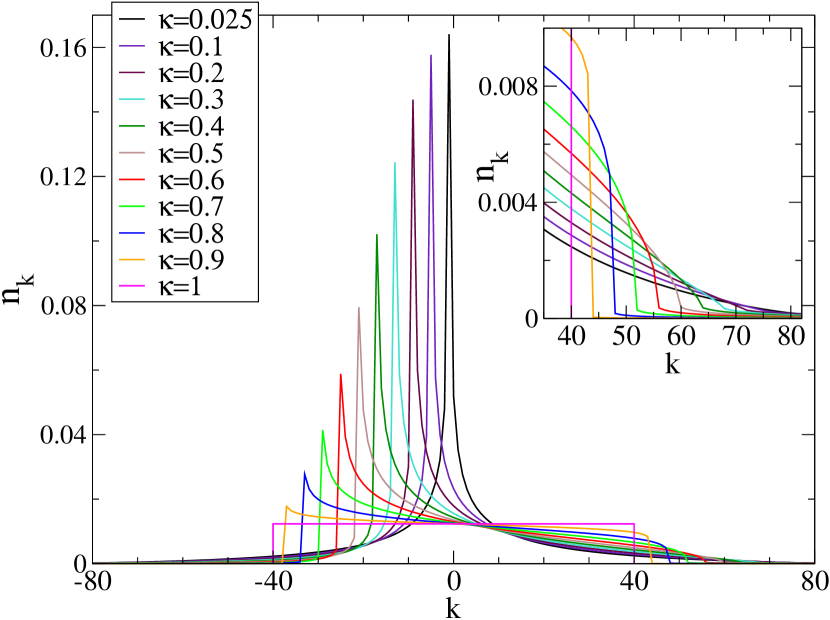
Figure 2: Momentum distribution function $n^{\kappa}_{81}(k)$ (i.e. $N=L=81$) for several statistical parameters $\kappa$ showing how the peak decreases with increasing $\kappa$ and becomes the Fermi discontinuity at $k=-k_{F}$. Inset: Zoom in the region $k_{F}<k<2k_{F}$ showing that the weak singularity at $k=2k_{F}$ for $\kappa=0$ becomes the discontinuity of the function at $k=k_{F}$ for $\kappa=1$.

Eq. (15) provides a representation of $\rho_{N}^{\kappa}(x)$ that can be easily used to derive the correlation function at finite $N$. In particular, for a small number of particles $N$ we have explicit expressions of $\rho_{N}^{\kappa}(x)$. For $N=3$, using the variable $t=2\pi x/L$, $0\leq t\leq 2\pi$, we find

$$\rho^{\kappa}_{N=3}(t)=\frac{1}{24\pi^{2}}\left[8\pi^{2}-\xi_{\kappa}(-15\xi_{\kappa}+8\pi t-2\xi_{\kappa}t^{2})+\xi_{\kappa}^{2}\cos 2t\right.$$

$$\left.+4(2\pi-\xi_{\kappa}(t+2))(2\pi-\xi_{\kappa}(t-2))\cos t+12\xi_{\kappa}(2\pi-\xi_{\kappa}t)\sin t\right]\,,$$ (33)

where $\xi_{\kappa}$ is defined by

$$\xi_{\kappa}=1-e^{i(1-\kappa)\pi}\,.$$ (34)

In the same manner and with the help of Mathematica, we can expand the determinant up to $N=11$. However, the formulas for general $\kappa$ are too long to be reported here. Larger values of $N$ can be easily worked out numerically. The small $N$ analytic expressions are then practical cases to check numerical calculations, asymptotic expansions etc. as we will extensively do in the following. For example, by fixing $t=2\pi$ in Eq. (33), and in the analogous ones not reported here, we can explicitely verify that $\rho^{\kappa}_{N=3}(L)=(1-\xi_{\kappa})^{2}\rho^{\kappa}_{N=3}(0)$ and $\rho^{\kappa}_{N=5}(L)=(1-\xi_{\kappa})^{4}\rho^{\kappa}_{N=5}(0)$ etc. in agreement with Eq. (11).

We now focus on the properties that can be derived from the numerical calculations of $\rho^{\kappa}_{N}(x)$. The correlation function in the real space has been already worked out numerically for several $\kappa$ in Ref. [7]. The agreement with the Fisher-Hartwig result Eq. (32) has been shown to be excellent for small $\kappa$. When $\kappa$ get closer to $1$, by using an harmonic fluid approach, it has been shown [10] that a second mode not captured by the Fisher-Hartwig, becomes important and is responsible for the right behavior at the fermionic point (these results were later rederived with a different approach [11]). Overall we can safely state that the main qualitative features of $\rho^{\kappa}_{N}(x)$ that can be extracted by numerics are well understood (with the important exception of fixing the amplitude of the second mode, see the discussion section for details). The same is not true for the momentum distribution function $n^{\kappa}_{N}(k)$ which has only been considered marginally [7, 10].

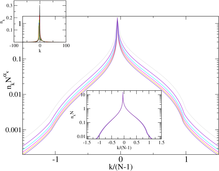
Figure 3: Scaling of the momentum distribution function $n^{\kappa=0.1}_{N}(k)$ with varying $N=21,41,61,81,101,121$. Upper inset: $n^{\kappa}_{N}(k)$ as function of $k$. Main Plot: Scaling of the peak by plotting $n^{\kappa}_{N}(k)N^{\alpha_{\kappa}}$ with $\alpha_{\kappa}=1/2+\kappa^{2}/2$ versus $k/(N-1)$. Central inset: $n^{\kappa}_{N}(k)N$ versus $k/(N-1)$ that gives the collapse for large $k$, and works well also for moderate values of $k$.

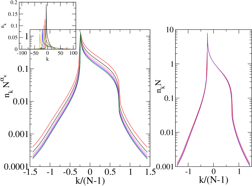
Figure 4: Scaling of the momentum distribution function $n^{\kappa=0.5}_{N}(k)$ with varying $N=21,41,61,81,101,121$. Upper inset: $n^{\kappa}_{N}(k)$ as function of $k$. Left Plot: Scaling of the peak by plotting $n^{\kappa}_{N}(k)N^{\alpha_{\kappa}}$ with $\alpha_{\kappa}=1/2+\kappa^{2}/2$ versus $k/(N-1)$. Right Plot: $n^{\kappa}_{N}(k)N$ versus $k/(N-1)$ that gives the collapse for large $k$.

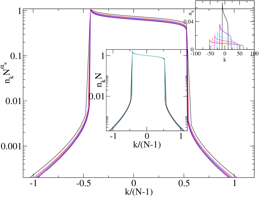
Figure 5: Scaling of the momentum distribution function $n^{\kappa=0.9}_{N}(k)$ with varying $N=21,41,61,81,101,121$. Upper inset: $n^{\kappa}_{N}(k)$ as function of $k$. Main Plot: Scaling of the peak by plotting $n^{\kappa}_{N}(k)N^{\alpha_{\kappa}}$ with $\alpha_{\kappa}=1/2+\kappa^{2}/2$ versus $k/(N-1)$. Central inset: $n^{\kappa}_{N}(k)N$ versus $k/(N-1)$ that gives the collapse for large $k$.

Here we fill this gap. For practical purposes we only consider the case of a periodic $\rho_{N}^{\kappa}(x)$, i.e. $\kappa=2m/(N-1)$, so that $n^{\kappa}_{N}(k)$ can be defined as the Fourier transform

$$n^{\kappa}_{N}(k)=\frac{1}{L}\int_{0}^{L}dxe^{2\pi ikx/L}\rho_{N}^{\kappa}(x)\,,$$ (35)

with $k$ integer. We calculated $n^{\kappa}_{N}(k)$ for all the values of $\kappa\in[0,1]$ that give an $L$-periodic $\rho_{N}^{\kappa}(x)$ for $N=L=21,41,61,81,101,121$ (higher values of $N$ could have been easily obtained, but the values considered are sufficient for our aims). The method is very simple: we calculated numerically $\rho_{N}^{\kappa}(x)$ for enough equispaced $x$’s and then we considered the fast Fourier transform of these data, obtaining very accurate results.

Let us first discuss the more natural question we can address with this method: how with changing $\kappa$ we can smoothly interpolate between the impenetrable boson and the free fermion momentum distribution functions. We remember to the reader that these two correlation functions are very different. The free fermion one is obviously a Fermi-Dirac distribution

$$n_{N}^{1}(k)=\cases{1/N&for $|k|<k_{F}$\,,\cr 1&for $|k|>k_{F}$\,,}$$ (36)

with $k_{F}=(N-1)/2$. Oppositely at $\kappa=0$, $n_{N}^{0}(k)$ has the characteristic of a strongly interacting system with a peak in $0$, going like $N^{-1/2}$ [27] and a large-momentum power-law tail [32, 33]. Both the limits are symmetric for $k\to-k$.

Fig. 2 shows $n_{81}^{\kappa}(k)$ (we take $N=81$ as a typical large enough value) for several $\kappa$ between 0 and 1 (the figure with all the possible $\kappa$ making $\rho_{N}^{\kappa}(x)$ periodic has too many curves to be readable). The peak at $k=0$ for $\kappa=0$ shifts backward at $k=-\kappa(N-1)/2$ and its height decreases from $N^{-1/2}$ to $N^{-\alpha_{\kappa}}$ with $\alpha_{k}=1/2+\kappa^{2}/2$. Both these features are encoded in the Fisher-Hartwig result Eq. (32). Approaching $\kappa=1$ this peak becomes the discontinuity at $k=-k_{F}$. However, the Fisher-Hartwig result only applies very close to this maximum value and cannot explain how the discontinuity at $k=k_{F}$ is produced, that instead is well understood from numerics. For bosons, it is known from the pioneering paper of Vaidya and Tracy [34] that not only $k=0$ is singular, but there are additional weaker singularities at all the points $k=2mk_{F}$ with $m$ integer. For example, at $k=\pm 2k_{F}$ the second derivative of $n_{N}^{0}(k)$ is divergent in the thermodynamic limit, but this singularity is so weak that is hardly seen in Fig. 2. Increasing $\kappa$, all these singularities move backward of $-\kappa(N-1)/2$. In particular, the first one at $2k_{F}$ moves at $2k_{F}-\kappa(N-1)/2$ and becomes sharper. This is emphasized by the inset of Fig. 2, where we zoom close to this region showing how the derivative of $n_{N}^{\kappa}(k)$ develops a larger discontinuity increasing $\kappa$, that becomes a discontinuity of the function itself for $\kappa=1$ at $k=k_{F}$.

We find that this mechanism to connect smoothly $\kappa=0$ to $\kappa=1$ is very interesting because of its simplicity. Furthermore we believe that it should be valid for the Lieb-Liniger model at arbitrary coupling, but unfortunately it is still impossible to have the analytic structure of the singularities in the general case. However, this structure is compatible with the results from the harmonic fluid approach [10, 11], where the amplitudes that fix the strength of the singularities are free parameters. Finally it is likely that this mechanism would be valid also for other models of interacting anyons.

There are other interesting features that can be extracted from our numerical calculations. We notice that, in contrast with the cases $\kappa=0,1$ the momentum distribution function is highly asymmetric. Increasing $\kappa$ the decay to the left of the peak becomes more rapid, while for $k>-\kappa(N-1)/2$, $n^{\kappa}_{N}(k)$ slowly develops a plateaux that becomes the Fermi sea at $\kappa=1$. However for value of $|k|$ larger than $k_{F}$ the momentum distribution function tends to restore the symmetry $k\to-k$. This is clear from Figs. 3, 4, and 5 where we plot $n^{\kappa}_{N}(k)$ for $\kappa=0.1,0.5,0.9$ in logarithmic scale to magnify the small values the functions take. In the following sections we will show rigorously that these tails follow a $k^{-4}$ power-law and are symmetric with respect to $k=0$ (the first asymmetric term is only at level $k^{-9}$ when $\kappa=2m/(N-1)$).

The three Figs. 3, 4, and 5 show also other interesting features of the momentum distribution function. We plot $n^{\kappa}_{N}(k)N^{\alpha_{\kappa}}$ with $\alpha_{\kappa}=1/2+\kappa^{2}/2$ as function of $k/(N-1)=2k/k_{F}$ that should show a perfect data collapse for all the values of $k$ well described by the Fourier transform of the asymptotic Fisher-Hartwig result valid for large $x$, and so close to the peak. It is evident from the figures, that the collapse is effective only extremely close to the peak. Oppositely for large $k$, the momentum distribution function is not expected to show any anomalous scaling and to be proportional to $1/N$ (this will be shown rigorously for large $k$ in the following sectionsL note the different normalizations of $n^{\kappa}_{N}(x)$). For this reason we also plot $Nn^{\kappa}_{N}(k)$ that in fact shows a good collapse of the data for large $k$. But not only: also for intermediate values of $k$ the various curves fall on the same “scaling” function.

4 Differential equation for $\rho^{\kappa}_{N}(x)$

An effective way of characterizing correlation functions for 1D strongly interacting systems is to find a differential equation that the correlation satisfies and from this extract the analytical properties of the solution. For the 1D impenetrable Bose gas this program started with the work of Jimbo et al. [35] proving that $\rho_{\infty}^{1}(x)$ (i.e. in the thermodynamic limit) satisfies a second order Painlevé differential equation of the V kind $P_{V}$. This result allowed to derive several terms in the asymptotic expansion for large distances [35]. Later Forrester and collaborators were able to show that also the finite $N$ correlation function $\rho^{0}_{N}(x)$ satisfies a $P_{VI}$ Painlevé equation and they pointed out useful connections with the theory of random matrices. Exploiting this connection, we show here that also the anyonic one-particle density matrix $\rho^{\kappa}_{N}(x)$ can be characterized via a second order non-linear differential equation $P_{VI}$.

The starting point is that $|\Psi^{1}_{0}(x_{1},x_{2},\cdots x_{N})|^{2}$ can be viewed as a probability distribution function for some class of random matrices [36] ($\Psi^{1}_{0}(x_{1},x_{2},\cdots x_{N})$ is the free fermion ground state). For periodic boundary condition, the appropriate matrix ensemble is the so called unitary circular ensemble [37], for which

$$|\Psi_{0}^{1}(x_{1},x_{2},\cdots,x_{N})|^{2}=\frac{1}{N!L^{N}}\prod_{1\leq j<k\leq N}4\sin[\pi(x_{j}-x_{k})/L]^{2}=\mbox{Ev(U(N))},$$ (37)

where Ev(U(N)) is the eigenvalue probability distribution function of unitary matrix $U(N)$ with uniform measure. Eq. (13) for $\rho^{\kappa}_{N}(x)$ can thus be interpreted as an average in the circular unitary ensemble

$$\rho^{\kappa}_{N}(t)=\langle\prod_{s=2}^{N}\frac{2}{\pi}A(t_{s}-t)\sin[(t_{s}-t)/2]\sin[t_{s}/2]\rangle_{\rm Ev(U(N))}.$$ (38)

It is known (see for instance Ref. [38] and references therein) that the averages in various random matrix ensembles are related to the Painlevé differential equations which are classified in six types: $P_{I},\cdots P_{VI}$. In the case of the average (38) it has been shown by Forrester et al. [25] that one can evaluate $\rho^{\kappa}_{N}$ via non-linear differential equation of $P_{VI}$ type. In fact, $\rho^{\kappa}_{2}(x),\rho^{\kappa}_{3}(x),\cdots\rho^{\kappa}_{N+1}(x)$ can be considered as a sequence of functions $\tau_{3}[1](u),\tau_{3}[2](u),\cdots\tau_{3}[N](u)$ (we introduced $\ln u=2ix$) which represents one of the so called $\tau$-function sequence occurring in the $P_{VI}$ systems. The first function of this sequence, $\tau_{3}[1](u)$, turns out to satisfy a Gauss hypergeometric equation, which admits two independent solutions. The parameters appearing in the hypergeometric equation do not depend on the anyonic parameter $\kappa$. The effect of the statistics is to select a particular solution in the bidimensional space of solutions of the hypergeometric equation. In other words, the anyonic statistics enters only in the determination of the boundary conditions. Using the so called Backlund transformations, which leave the form of the $P_{VI}$ equations unchanged, one can systematically construct all the $\tau_{3}[N]$ function from the $\tau_{3}[1]$ and verify that the form of the corresponding differential equations do not depend on the statistics. Specifically, the function $\sigma^{\kappa}_{N}(u)$ (directly related to $\tau_{3}[N](u)$)

$$\sigma^{\kappa}_{N}(u)=u(u-1)\ln\rho^{\kappa}_{N}(x(u)),\qquad x(u)=\frac{\ln u}{2i},$$ (39)

satisfies the following second order differential equation

$$u^{2}(u-1)^{2}\left[\frac{d^{2}}{du^{2}}\sigma^{\kappa}_{N}(u)\right]^{2}+4\left[\sigma_{N}(u)-(u-1)\frac{d}{du}\sigma^{\kappa}_{N}(u)+1\right]\times$$ (40)

$$\times\left[\sigma^{\kappa}_{N}(u)\frac{d}{du}\sigma^{\kappa}_{N}(u)-u\left(\frac{d}{du}\sigma^{\kappa}_{N}(u)\right)^{2}-\frac{N^{2}-1}{4}\left(\sigma^{\kappa}_{N}(u)-(u-1)\frac{d}{du}\sigma^{\kappa}_{N}(u)\right)\right]=0,$$

that in fact does not depend explicitely on the anyonic parameter $\kappa$. The study of the boundary conditions for general values of $\kappa$ is missing in Ref. [25], where only the bosonic and fermionic cases ($\kappa=0,1$) have been discussed. The general $\kappa$ dependence of the boundary conditions ($\xi_{\kappa}$ is defined in Eq. (34))

$$\lim_{u\to 1}\sigma_{N}(u)\sim\frac{N^{2}-1}{12}(u-1)^{2}-\left(\frac{N^{2}-1}{24}+i\xi_{\kappa}\frac{N(N^{2}-1)}{48\pi}\right)(u-1)^{3}\,,$$ (41)

are derived by expanding $\rho^{\kappa}_{N}(t=2\pi x/L)$ in power of $x$. Let us show how to derive this result. Using Eqs. (8) and (34), Eq. (13) can be written as

$$\rho^{\kappa}_{N}(t)=\frac{1}{N!}\prod_{s=2}^{N}\left(\int_{0}^{2\pi}dt_{s}-\xi_{\kappa}\int_{0}^{t}dt_{s}\right)\prod_{s=2}^{N}\frac{2}{\pi}\sin[(t_{s}-t)/2]\sin[t_{s}/2]$$

$$\qquad\qquad\qquad\qquad\qquad\times\prod_{2\leq i<j\leq N}4\sin[(t_{j}-t_{i})/2]^{2}.$$ (42)

Expanding the above expression in powers of $\xi_{\kappa}$, $\rho_{N}^{\kappa}(t)$ is expressed in terms of the $(n+1)$-particle density matrices $\rho^{1}_{(n,N)}(t,t_{2},\cdots t_{n+1};0,t_{2},\cdots t_{n+1})$ of a system of $N$ free fermions

$$\rho^{\kappa}_{N}(t)=\rho^{1}_{N}(t)+$$

$$\qquad+\sum_{n=1}^{N}\frac{(-\xi_{\kappa})^{n}}{n!}\int_{0}^{t}dt_{2}\int_{0}^{t}dt_{3}\cdots\int_{0}^{t}dt_{n+1}\rho^{1}_{(n,N)}(t,t_{2},\cdots t_{n+1};0,t_{2},\cdots t_{n+1})\,,$$ (43)

The $n-$th term of the above expansion is proportional to the $n-$th power of $t$. Using the Wick theorem, the $(n+1)$-particles density matrix $\rho^{1}_{N}(t,t_{2},\cdots t_{n+1};0,t_{2},\cdots t_{n+1})$ is expressed as a products of one-particle density matrices $\rho^{1}_{N}$. Using

$$\rho^{1}_{N}(x)=\frac{\sin(N\pi x/L)}{N\sin(\pi x/L)},$$ (44)

the $2$ free fermions density matrix $\rho^{1}_{(2,N)}(t,t_{2};0,t_{2})$ is

$$\rho^{1}_{(2,N)}(x,x_{2};0,x_{2})=\rho^{1}_{N}(x)\rho^{1}_{N}(0)-\rho^{1}_{N}(x_{2})\rho^{1}_{N}(x-x_{2})=$$

$$\quad=\frac{\sin(N\pi x/L)}{N\sin\pi x/L}-\frac{\sin(N\pi x_{2}/L)}{N\sin(\pi x_{2}/L)}\frac{\sin(N\pi(x-x_{2})/L)}{N\sin(\pi(x-x_{2})/L)}\,.$$ (45)

At the first order in $\xi_{\kappa}$, we have

$$\rho_{N}(x)=\frac{\sin(N\pi x/L)}{N\sin(\pi x/L)}$$

$$\qquad-\frac{\xi_{\kappa}}{L}\int_{0}^{x}dx_{2}N\left[\frac{\sin(N\pi x/L)}{\sin(\pi x/L)}-\frac{\sin(N\pi x_{2}/L)}{\sin(\pi x_{2}/L)}\frac{\sin(N\pi(x-x_{2})/L)}{\sin(\pi(x-x_{2})/L)}\right]+O(\xi_{\kappa}^{2}),$$ (46)

which gives

$$\lim_{x\to 0}\rho_{N}^{\kappa}(x)=1-\frac{N^{2}-1}{6}(\pi x/L)^{2}+\xi_{\kappa}\frac{N(N^{2}-1)}{18\pi}(\pi x/L)^{3},$$ (47)

that is equivalent to Eq. (41).

Note that Eq. (42) shows explicitely that the non real (i.e. the imaginary parts) terms in $\rho^{\kappa}_{N}(x)$ come from $\xi_{\kappa}$ alone. This is suggestive for an artificial interpolation between bosons and fermions that does not require complex phases.

5 Short distance and large momentum expansions

Starting from the work of Jimbo et al. [35] differential equations satisfied by correlation functions become one of the most powerful tool to obtain asymptotic expansions. Eq. (40) joined with the boundary condition (41) allows to obtain the small $x$ expansion of $\rho^{\kappa}_{N}(x)$, on the same line of Ref. [39] for impenetrable bosons. In fact, by substituting a small $x$ power series for $\rho^{\kappa}_{N}(x)$ into the differential equation, we obtain equations which define all but one of the coefficients. In particular the resulting equation for the coefficient $x^{3}$ vanishes identically, and to fix this parameter we require the boundary condition (41). With the help of Mathematica, we found straightforward to obtain the first 25 terms of $\rho^{\kappa}_{N}(x)$, but it would require far too much space to exhibit all these here. In the variable $t=2\pi x/L$ up to order $t^{10}$ we find

$$\rho^{\kappa}_{N}(x)=1-\frac{N^{2}-1}{2^{2}6}t^{2}+\xi_{\kappa}\frac{N(N^{2}-1)}{2^{3}18\pi}t^{3}$$ (48)

$$\qquad+\frac{(3N^{2}-7)(N^{2}-1)}{2^{4}360}t^{4}-\xi_{\kappa}\frac{N(11N^{2}-29)(N^{2}-1)}{2^{5}2700\pi}t^{5}$$

$$\qquad-\frac{(3N^{4}-18N^{2}+31)(N^{2}-1)}{2^{6}15120}t^{6}-\xi_{\kappa}\frac{N(183N^{4}-1210N^{2}+2227)(N^{2}-1)}{2^{7}1587600\pi}t^{7}$$

$$\qquad+\frac{(N^{2}-1)[(15N^{6}-165N^{4}+717N^{2}-1143)\pi^{2}+56N^{2}(N^{2}-4)\xi_{\kappa}^{2}]}{2^{8}5443200\pi^{2}}t^{8}$$

$$\qquad-\xi_{\kappa}\frac{N(-22863+13867N^{2}-3017N^{4}+253N^{6})(N^{2}-1)}{2^{9}142884000\pi}t^{9}-$$

$$\qquad-\frac{N^{2}-1}{2^{10}62868960000\pi^{2}}[525(3N^{8}-52N^{6}+410N^{4}-1636N^{2}+2555)\pi^{2}+$$

$$\qquad 88N^{2}(489N^{6}-4606N^{4}+12761N^{2}-8644)\xi_{\kappa}^{2})t^{10}.$$

In the bosonic case, $\kappa=0$ ($\xi_{\kappa}=2$), we find the result obtained in Ref. [39]. In the fermionic case, $\kappa=1$ ($\xi_{\kappa}=0$), the above formula gives the small $x$ expansion of $\rho^{1}_{N}(x)$ of Eq. (44).

Note that the dependence of the previous expansion up to the order $t^{7}$ is trivial, in the sense that the even terms are the same as for bosons, while the odd ones only get a global factor $\xi_{\kappa}$. While the latter property is true at all the orders we calculated, the former has a non-trivial $\xi_{\kappa}$ dependence that firstly shows up in the term $t^{8}$ with a factor proportional to $\xi_{\kappa}^{2}$. Higher powers in $t$ show also higher powers of $\xi_{\kappa}^{2}$.

5.1 Large moment expansion

Because of the periodicity properties of $\rho^{\kappa}_{N}(x)$ in Eq. (11), the momentum distribution function cannot be defined simply as a Fourier series. Its definition should be changed according to (for convenience we also introduced a factor $1/N$ compared to the definition in Eq. (35))

$$\rho^{\kappa}_{N}(x)=\frac{1}{N}\sum_{n=-\infty}^{\infty}n^{\kappa}_{N}(k)\exp\left[-2\pi i(k+\delta_{\kappa})\frac{x}{L}\right],$$ (49)

where the shift $\delta_{\kappa}$ is defined by

$$\delta_{\kappa}=\left\{1+(\kappa-1)\frac{N-1}{2}\right\},$$ (50)

and $\{x\}=x-[x]$ stands for the non-integer part of $x$. This shift in the definition does not matter when $\rho^{\kappa}_{N}(x)$ is periodic, i.e. for $\kappa=2m/(N-1)$, when $\delta_{\kappa}=0$. Inverting Eq. (49), the momentum distribution function is

$$n^{\kappa}_{N}(k)=\frac{N}{L}\int_{0}^{L}dx\exp\left[2\pi i(k+\delta_{\kappa})\frac{x}{L}\right]\rho^{\kappa}_{N}(x),$$ (51)

that gives the probability occupation of the states with momentum $2\pi(k+\delta_{\kappa})/L$. For a small number of particles it is possible to obtain close expressions of $n^{\kappa}_{N}(k)$. For $N=3$, from Eq. (33) we have (we stress that this formula is valid only for $0<\kappa<1$)

$$n^{\kappa}_{3}(k)=\frac{4\cos^{2}\left(\pi\kappa/2\right)\left(4\sin\left(\pi\kappa\right)p_{2}(k,\kappa)+\pi p_{7}(k,\kappa)\right)}{\pi^{3}\left(-4+k^{2}+2k\kappa+\kappa^{2}\right)\left(-k+k^{3}-\kappa+3k^{2}\kappa+3k\kappa^{2}+\kappa^{3}\right)^{3}},$$ (52)

where the $p_{2}(k,\kappa)$ and $p_{7}(k,\kappa)$ are respectively polynomials of order $2$ and $7$ in $k$

$$p_{2}(k,\kappa)=7k^{2}+14k\kappa-1+7\kappa^{2},$$

$$p_{7}(k,\kappa)=3k^{7}+21k^{6}\kappa+7k^{5}(9\kappa^{2}-2)+35k^{4}\kappa(3\kappa^{2}-2)+7k^{3}(1-20\kappa^{2}+15\kappa^{4})+$$

$$\;+7k^{2}\kappa(3-20\kappa^{2}+9\kappa^{4})+k(4+21\kappa^{2}-70\kappa^{4}+21\kappa^{6})+\kappa(4+7\kappa^{2}-14\kappa^{4}+3\kappa^{6}).$$

For $\kappa=0$, this reduces to the bosonic distribution function $n^{0}_{3}(k)$ [39]

$$n^{0}_{3}(0) = \frac{1}{3}+\frac{35}{2\pi^{2}},\quad n^{0}_{3}(\pm 1)=\frac{1}{3},\quad n^{0}_{3}(\pm 2)=\frac{35}{36\pi^{2}},$$

$$n^{0}_{3}(k) = \frac{2(3k^{7}-14k^{5}+7k^{3}+4k)}{(-4+k^{2})(-k+k^{3})^{3}\pi^{2}},\qquad|k|>2,$$ (53)

and for $\kappa=1$ to the Fermi distribution

$$n^{1}_{3}(0)=n^{1}_{3}(\pm 1)=1,\qquad n^{1}_{3}(k)=0\quad|k|>1\,.$$ (54)

The close expression for $n^{\kappa}_{5}(k)$ and $n^{\kappa}_{7}(k)$ are too long to be reported here.

5.2 Large momentum asymptotic expansions

From the exact solutions for different values of $N$ ($N=3,5,7$) and $\kappa$, we can study the behavior of the distribution of large momenta $k\gg 1$ by studying the asymptotic of the function $n^{\kappa}_{N}(k-\delta_{\kappa})$. For $N=3$ we find

$$n^{\kappa}_{3}(n-\delta_{\kappa})=\frac{6\cos^{2}(\pi\kappa/2)}{\pi^{2}k^{4}}+\frac{14\cos^{2}(\pi\kappa/2)}{\pi^{2}k^{6}}+\frac{22\cos^{2}(\pi\kappa/2)}{\pi^{2}k^{8}}+\frac{56\cos^{2}(\pi\kappa/2)\sin(\pi\kappa)}{\pi^{3}k^{9}}$$

$$\qquad\qquad+\frac{30\cos^{2}(\pi\kappa/2)}{\pi^{2}k^{10}}+\frac{384\cos^{2}(\pi\kappa/2)\sin(\pi\kappa)}{\pi^{3}k^{11}}+O(k^{-12}).$$ (55)

Note that, for generic values of $\kappa$, we have odd terms appearing in the asymptotic expression (55). As another illustrative example of the large $k$ behavior of $n^{\kappa}_{N}(k)$, we give the large $k$ expansions for $n^{0}_{5}(k)$, $n^{1/2}_{5}(k)$ and $n^{1/3}_{5}(k)$

$$n^{0}_{5}(k) = \frac{50}{\pi^{2}k^{4}}+\frac{410}{\pi^{2}k^{6}}+\frac{2570}{\pi^{2}k^{8}}+\frac{14234}{k^{10}}+0(k^{-12}),$$

$$n^{1/2}_{5}(k) = \frac{25}{\pi^{2}k^{4}}+\frac{205}{\pi^{2}k^{6}}+\frac{1285}{\pi^{2}k^{8}}+\frac{4900}{\pi^{3}k^{9}}+\frac{7117}{\pi^{2}k^{10}}+\frac{150960}{\pi^{3}k^{11}}+0(k^{-12}),$$

$$n^{1/3}_{5}(k+1/3) = \frac{75}{2\pi^{2}k^{4}}+\frac{615}{2\pi^{2}k^{6}}+\frac{3855}{2\pi^{2}k^{8}}+\frac{3675\sqrt{3}}{\pi^{3}k^{9}}+\frac{21351}{2\pi^{2}k^{10}}+0(k^{-11}).$$ (56)

For $N=7$ the large $k$ expansions for different values of $\kappa$ (giving periodic $\rho^{\kappa}_{N}(x)$) take the form

$$n^{0}_{7}(k) = \frac{196}{\pi^{2}k^{4}}+\frac{3332}{\pi^{2}k^{6}}+\frac{44604}{\pi^{2}k^{8}}+\frac{540820}{\pi^{2}k^{10}}+0(k^{-12}),$$

$$n^{1/3}_{7}(k) = \frac{147}{\pi^{2}k^{4}}+\frac{2499}{\pi^{2}k^{6}}+\frac{33453}{\pi^{2}k^{8}}+\frac{86436\sqrt{3}}{\pi^{3}k^{9}}+\frac{405615}{\pi^{2}k^{10}}+\frac{5768280\sqrt{3}}{\pi^{3}k^{11}}+0(k^{-12}),$$

$$n^{2/3}_{7}(k) = \frac{49}{\pi^{2}k^{4}}+\frac{833}{\pi^{2}k^{6}}+\frac{11151}{\pi^{2}k^{8}}+\frac{28812\sqrt{3}}{\pi^{3}k^{9}}+\frac{135205}{\pi^{2}k^{10}}+\frac{1922760\sqrt{3}}{\pi^{3}k^{11}}+0(k^{-12}).$$

The large $k$ expansion of $n^{\kappa}_{N}(k)$ for general values of $\kappa$ and $N$ can be obtained by means of the Mellin transform. Given a function $f(x)$, the Mellin transform is defined as

$$\phi(s)=\int_{0}^{\infty}dxx^{s-1}f(x).$$ (57)

whose inverse is

$$f(x)=\frac{1}{2\pi i}\int_{c-i\infty}^{c+\infty}dsx^{-s}\phi(s),$$ (58)

where the above notation implies a contour integral taken over a vertical axis in the complex plane in the corresponding fundamental strip.

The Mellin transform establishes a direct mapping between the asymptotic expansion of a function $f(x)$ near $x=0$ and the set of singularities of the transform $\phi(s)$ in the complex plane. This technique has been already applied in Ref. [39] to the bosonic case (i.e. $\kappa=0$).

The asymptotic expansions we compute from the small $N$ exact solutions suggest the following general large $k$ expansion for $n^{\kappa}_{N}(k-\delta_{\kappa})$

$$n^{\kappa}_{N}(k-\delta_{\kappa})\sim\frac{a^{\kappa}_{1}}{k^{4}}+\frac{b^{\kappa}_{1}}{k^{5}}+\frac{a^{\kappa}_{2}}{k^{6}}+\frac{b^{\kappa}_{2}}{k^{7}}+\frac{a^{\kappa}_{3}}{k^{8}}+\frac{b^{\kappa}_{3}}{n^{9}}+\cdots$$ (59)

We use the Mellin transforms of the $\cos(2\pi nx)$ and $\sin(2\pi nx)$ functions

$$\cos(2\pi kx)=\frac{1}{2\pi i}\int_{c-i\infty}^{c+i\infty}ds\Gamma(s)\cos(\pi s/2)(2\pi nx)^{-s}\quad 0<c<1,$$

$$\sin(2\pi kx)=\frac{1}{2\pi i}\int_{c-i\infty}^{c+i\infty}ds\Gamma(s)\sin(\pi s/2)(2\pi nx)^{-s}\quad-1<c<1.$$ (60)

Plugging Eq. (59) and Eq. (60) in Eq. (49), we have

$$\mbox{Re}\left[\rho^{\kappa}_{N}\right](x) = \frac{1}{L}n^{\kappa}_{N}(0)+\frac{1}{2\pi i}\int_{c-i\infty}^{c+i\infty}ds\,\Gamma(s)\cos(\pi s/2)(2\pi x)^{-s}g(s),$$

$$\mbox{Im}\left[\rho^{\kappa}_{N}\right](x) = \frac{1}{2\pi i}\int_{c-i\infty}^{c+i\infty}ds\,\Gamma(s)\sin(\pi s/2)(2\pi x)^{-s}g(s),$$ (61)

where

$$g(s)=g_{\mbox{even}}(s)+g_{\mbox{odd}}(s)=\sum_{j=1}^{\infty}a^{\kappa}_{j}\zeta(2j+2+s)+\sum_{j=1}^{\infty}b^{\kappa}_{j}\zeta(2j+3+s),$$ (62)

with $\Gamma(x)$ and $\zeta(x)$ the Gamma and Riemann function respectively. By closing the contour of (61) on the left, the above integral is given by the sum of the residues of the functions $\Gamma(s)\cos(\pi s/2)g(s)$ and $\Gamma(s)\sin(\pi s/2)g(s)$. The poles of these functions are all simple and located at the points $s=0,-2,-3,-4,-5,\cdots$ for the integral with the cosine and $s=-2,-3,-4\cdots$ for the integral with the sine.

In the integral (61) the singularities arise for $s=-2m$, $m\geq 0$ from the $\Gamma(s)\cos(\pi s/2)$ function and from the $m-1$-th term of the sum $g_{\mbox{odd}}(s)$ while for $s=-(2m+1)$, $m\geq 1$, from the Riemann function appearing in $m$-th term of the sum $g_{\mbox{even}}(s)$. Defining the function $f_{c}(z)$ as

$$f_{c}(-2m)=\mbox{Res}[\Gamma(s)\cos(\pi s/2)g(s),s=-2m],\qquad m\geq 1,$$ (63)

the resulting expansion then reads ($t=2\pi x/L$)

$$\mbox{Re}[\rho^{\kappa}_{N}](x)=1-\frac{f_{c}(-2)}{4N}t^{2}+\frac{4\pi a^{\kappa}_{1}}{6N}t^{3}+\frac{f_{c}(-4)}{16N}t^{4}-\frac{\pi a^{\kappa}_{2}}{120N}t^{5}$$ (64)

$$-\frac{f_{c}(-6)}{64N}t^{6}+\frac{\pi a^{\kappa}_{3}}{5040N}t^{7}+\frac{f_{c}(-8)}{256N}t^{8}-\frac{\pi a^{\kappa}_{4}}{362880N}t^{9}+O(t^{10}).$$ (65)

The coefficients of the even terms in the above expansion contain then all the terms of the sums in $g(s)$. Note that the term arising from the residue at $s=0$ combines with $n^{\kappa}_{N}(0)/L$ to give $\rho^{\kappa}_{N}(0)=1$. The first terms for example are

$$f_{c}(-2) = 4g(-2),$$

$$f_{c}(-4) = \frac{4}{3}\left(g_{\mbox{even}}(-4)+\sum_{j=2}^{\infty}b^{\kappa}_{j}\zeta(2j+3+s)\right)+\frac{25}{9}b^{\kappa}_{1},$$ (66)

Comparing Eq. (48) with Eq. (65), we have the $a^{\kappa}_{j}$ coefficients

$$a^{\kappa}_{1} = \frac{N^{2}(N^{2}-1)}{24\pi^{2}}\mbox{Re}[\xi_{\kappa}],$$

$$a^{\kappa}_{2} = \frac{N^{2}(N^{2}-1)(-29+11N^{2})}{720\pi^{2}}\mbox{Re}[\xi_{\kappa}],$$

$$a^{\kappa}_{3} = \frac{N^{2}(N^{2}-1)(2227-1210N^{2}+183N^{4})}{40320\pi^{2}}\mbox{Re}[\xi_{\kappa}],$$

$$a^{\kappa}_{4} = \frac{N^{2}(N^{2}-1)(-22863+13867N^{2}-3017N^{4}+253N^{6}))}{201600\pi^{2}}\mbox{Re}[\xi_{\kappa}].$$ (67)

For $N=3,5,7$ we recover the exact results given above.

In an analogous way the coefficients $b_{j}^{\kappa}$ are derived from the sine integral. Here the singularities for $s=-2m$, $m\geq 2$, arise from the Riemann function appearing in $(m-1)$-th term of the sum $g_{\mbox{odd}}(s)$ while the singularities for $s=-(2m+1)$, $m\geq 1$, arise from the $\Gamma(s)\sin(\pi s/2)$ function and from the $m$-th term of the sum $g_{\mbox{even}}(s)$. Defining the function $f_{s}(z)$ as

$$f_{s}(-2m-1)=\mbox{Res}[\Gamma(s)\sin(\pi s/2)g(s),s=-2m-1],\qquad m\geq 1,$$ (68)

we find the following expansion ($t=2\pi x/L$)

$$\mbox{Im}[\rho^{\kappa}_{N}](x)=\frac{f_{s}(-3)}{8N}t^{3}+\frac{\pi b^{\kappa}_{1}}{32N}t^{4}+\frac{f_{s}(-5)}{32N}t^{5}-\frac{\pi b^{\kappa}_{2}}{720N}t^{6}+$$

$$+\frac{f_{s}(-7)}{128N}t^{7}+\frac{\pi b^{\kappa}_{3}}{20160N}t^{8}+\frac{f_{c}(-9)}{512N}t^{9}-\frac{\pi b^{\kappa}_{4}}{907200N}t^{10}+O(t^{11}).$$ (69)

Finally, comparing Eq. (48) with Eq. (69), we have the coefficients $b^{\kappa}_{j}$

$$b^{\kappa}_{1} = b^{\kappa}_{2}=0,$$

$$b^{\kappa}_{3} = -\frac{56N^{3}(N^{2}-1)(4-5N^{2}+N^{4})}{34560\pi^{3}}\mbox{Im}[\xi_{\kappa}^{2}],$$

$$b^{\kappa}_{4} = -\frac{N^{3}(N^{2}-1)^{2}(8644-4117N^{2}+489N^{4}))}{201600\pi^{3}}\mbox{Im}[\xi_{\kappa}^{2}].$$ (70)

We have shown that the first odd term appearing in the large $k$ expansion of $n^{\kappa}_{N}(k)$ is the one at the order $k^{-9}$. Again, one can verify the above values match with the exact results for a small number of particles ($N=5,7$). These odd terms are very important because they represent the onset of the asymmetry of $n^{\kappa}_{N}(k)$ for large $k$. Note that the first non-vanishing odd term is $k^{-9}$ because in the expansion (48) the first non trivial terms shows up at $t^{8}$.

6 Large $k$ asymptotics for a finite interaction anyonic gas

In the case of the Bose gas, it is well understood [33] that the $k^{-4}$ tail of the momentum distribution function (and the corresponding small $x$ behavior) are not a prerogative of the impenetrable limit, but are a signature of the delta-function interaction and so are general features of the Lieb-Liniger model, as confirmed by direct numerical calculations [24]. It is easy to generalize this result to the anyonic case and find the same result.

In order to prove this, we need to briefly introduce the Bethe Ansatz solution of the Lieb-Liniger gas [3, 4]. For finite arbitrary coupling $c$, the eigenstates $\Psi^{\kappa}_{c}(x_{1},\dots,x_{N})$ can be written as [3]

$$\Psi^{\kappa}_{c}(x_{1},\dots,x_{N})=\Phi^{\kappa}(x_{1},\dots,x_{N})\Psi^{0}_{\tilde{c}}(x_{1},\dots,x_{N})\,,$$ (71)

where the phase function

$$\Phi^{\kappa}(x_{1},\dots,x_{N})=e^{-i\pi N(N-1)\kappa/4}\prod_{q>p}e^{i\pi\kappa\epsilon(x_{q}-x_{p})/2}\,,$$ (72)

encodes all the statistic dependence of the wave functions (we adapted the anyon convention used in Ref. [3] to ours). In this way the problem is equivalent to find the bosonic wave-function $\Psi^{0}_{\tilde{c}}(x_{1},\dots,x_{N})$ (in fact this method is usually called Anyon-Boson mapping, oppositely to the Anyon-Fermion mapping exploited in the rest of the work and valid only for $c=\infty$).

Kundu [3] showed that the bosonic coupling ${\tilde{c}}$ is ${\tilde{c}}=c/\cos(\pi\kappa/2)$ and so all the thermodynamic quantities only depends on this effective bosonic coupling. For example, limiting to the $L$-periodic cases, we can write the ground-state energy per particle as

$$\frac{E_{0}}{N}\equiv\rho_{0}^{2}e(\gamma,\kappa)=\rho_{0}^{2}({\tilde{\gamma}},\kappa=0)\,,$$ (73)

where $\rho_{0}=N/L$ is the mean-density, $\gamma=c/\rho_{0}$, analogously ${\tilde{\gamma}}$, and $e(\gamma,\kappa)$ is implicitly defined above. For $\kappa=0$, $e(\gamma,0)$ has not a close analytical expression, but it is well-known and tabulated [20].

In Ref. [33] the large $k$ behavior of the momentum distribution function for the bosonic Lieb-Liniger model was simply derived by the fact that the wave function at the point of contact of any two particles undergo a kink in the derivative proportional to the value of the eigenfunction itself. The modification in the anyonic case is a straightforward consequence of Eq. (71): only the imaginary part of the eigenfunction $\Psi^{\kappa}_{c}(x_{1},\dots,x_{N})$ is discontinuous at a point of contact (and being odd does not contribute to the leading term for large $k$, in analogy with the well-known fermionic case), while the real part is continuous and its derivative has the kink of the corresponding boson wave-function $\Psi^{0}_{\tilde{c}}(x_{1},\dots,x_{N})$. Consequently the coefficient of the large momentum tail is the same as the one of the bosonic model at coupling ${\tilde{c}}$, i.e. [33]

$$n^{\kappa}_{N\gg 1}(k\to\infty) = \cos^{2}(\pi\kappa/2){\tilde{\gamma}}^{2}\frac{de(\tilde{\gamma},\kappa=0)}{d\tilde{\gamma}}\left(\frac{N}{2\pi k}\right)^{4}$$ (74)

$$= \cos(\pi\kappa/2)\gamma^{2}\frac{de(\gamma,\kappa)}{d\gamma}\left(\frac{N}{2\pi k}\right)^{4}\,,$$

where we adapt the result of Ref. [33] to the normalization $\rho_{N}^{\kappa}(0)=1$. Considering the large $\gamma$ expansion $e^{\prime}(\gamma,\kappa)=\cos(\pi\kappa/2)4\pi^{2}/(3\gamma^{2})$ [4] we agree with the result of the previous section in the impenetrable limit.

7 Discussions

In this paper we presented a systematic study of the momentum distribution function and of the one-particle reduced density matrix of the anyonic generalization of the Lieb-Liniger model, obtaining the first full analytic description of the crossover from bosons to fermions for a strongly interacting model of anyons. Particular attention has been devoted to the large momentum and small distance behavior that can be analytical obtained with a proper generalization of the methods employed for impenetrable bosons. In the complementary regime (large distance) we obtained the leading term by applying the Fisher-Hartwig conjecture. Corrections to the leading behavior have been investigated numerically. In this regime, we find the evidence that the second mode of the harmonic fluid approach [10] plays a fundamental role in describing the correct crossover to the free fermionic regime close to the point $k=k_{F}$. This calls for further analytical studies of the singularities of the momentum distribution function. Several techniques could be used to tackle this problem. In the bosonic case, the systematic large $x$ expansion has been mainly exploited via the solution of the second order differential equation $P_{V}$ [35, 39], but this required the knowledge of the proper boundary condition for large $x$ that was available only from the mapping to the lattice XX model [34] whose equivalent is not yet known for anyons. An alternative method, that has been applied successfully to bosons [40], would be to consider the replica approach. Work in this direction are in progress. Another effective way to obtain the asymptotics (maybe even beyond the impenetrable limit) would be the approach of Ref. [41].

The knowledge of the anyonic correlation functions beyond the impenetrable limit is instead still very limited. Only the power-law structure (and the corresponding singularities) are known from the harmonic fluid approach [10] (or equivalently from conformal field theory [11]). A general approach would be to generalize the quantum inverse scattering methods for bosons [23] to anyons and then to mix integrability and numerics to get the full correlation functions from the form-factors (on the line of Ref. [24]). But this is a very ambitious and long project. However, there is an interesting regime where this is maybe not necessary: in Ref. [4], exploiting the correspondence ${\tilde{c}}=c/\cos(\pi\kappa/2)$ [3], it has been argued that for $1<\kappa<2$ the corresponding bosonic model is attractive, independently of the coupling constant $c$. The attractive Bose gas is known to form bound-states whose wave-functions are known with exponential precision [42]. This allows the explicit analytic calculation of the correlation functions [43], that can eventually have some interpretation in anyonic language.

References

References

-
[1]
J. Leinaas, J. Myrheim, Nuovo Cimento B 37, 1(1977);
F. Wilczek, Phys. Rev. Lett. 48, 1144 (1982);
F. Wilczek, Fractional Statistics and Anyon Superconductivity, (World Scientific, Singapore 1990). - [2] S. Das Sarma, M. Freedman, C. Nayak, S. H. Simon, and A. Stern, arXiv:0707.1889, and references therein.
- [3] A. Kundu, Phys. Rev. Lett. 83, 1275 (1999) [hep-th/9811247].
-
[4]
M. T. Batchelor, X. W. Guan, N. Oelkers,
Phys. Rev. Lett. 96, 210402 (2006) [cond-mat/0603643];
M. T. Batchelor, X. W. Guan, J.S.-He, J. Stat. Mech. (2007) P03007 [cond-mat/0611450]. - [5] M. T. Batchelor, X. W. Guan, Phys. Rev. B 74 195121 (2006) [cond-mat/0606353].
- [6] M. D. Girardeau, Phys. Rev. Lett. 97, 210401 (2006) [cond-mat/0604357].
- [7] R. Santachiara, F. Stauffer, and D. Cabra, J. Stat. Mech. (2007) L05003 [cond-mat/0610402].
- [8] J. Zhu and Z. D. Wang, Phys. Rev. A 53, 600 (1992).
- [9] M. T. Batchelor and X. W. Guan, Laser Phys. Lett. 4 77 (2007) [cond-mat/0608624].
- [10] P. Calabrese and M. Mintchev, Phys. Rev. B 75, 233104 (2007) [cond-mat/0703117].
- [11] O. I. Patu, V. E. Korepin and D. V. Averin, J. Phys. A 40 14963 (2007) [0707.4520].
- [12] D. V. Averin and J. A. Nesteroff, Phys. Rev. Lett. 99, 096801 (2007) [0704.0439];
-
[13]
A. Liguori, M. Mintchev, and L. Pilo,
Nucl. Phys. B 569, 577 (2000) [hep-th/9906205];
A. Liguori and M. Mintchev, Commun. Math. Phys. 169, 635 (1995) [hep-th/9403039]. -
[14]
N. Ilieva and W. Thirring, Eur. Phys. J. C 6, 705 (1999) [hep-th/9808103];
N. Ilieva and W. Thirring, Theor. Mat. Phys. 121, 1294 (1999) [math-ph/9906020]. -
[15]
E.-A. Kim, M. J. Lawler, S. Vishveshwara, E. Fradkin,
Phys. Rev. Lett. 95, 176402 (2005) [cond-mat/0507428];
E.-A. Kim, M. J. Lawler, S. Vishveshwara, E. Fradkin, Phys. Rev. B 74, 155324 (2006) [cond-mat/0604325];
A. Lopez and E. Fradkin, Phys. Rev. B. 59, 15323 (1999) [cond-mat/9810168]. -
[16]
A. Feiguin, S. Trebst, A. W. W. Ludwig, M. Troyer, A. Kitaev, Z. Wang,
and M. H. Freedman, Phys. Rev. Lett. 98, 160409 (2007) [cond-mat/0612341];
S. Trebst, E. Ardonne, A. Feiguin, D. A. Huse, A. W. W. Ludwig, M. Troyer, arXiv:0801.4602 - [17] M. Greiter, arXiv:0707.1011.
- [18] R.-G. Zhu and A.-M. Wang, arXiv:0712.1264.
- [19] S. Ouvry, arXiv:0712.2174.
-
[20]
E. H. Lieb and W. Liniger, Phys. Rev. 130, 1605 (1963);
E. H. Lieb, Phys. Rev. 130, 1616 (1963). -
[21]
H. Moritz, T. Stoferle, M. Köhl and T. Esslinger,
Phys. Rev. Lett. 91, 250402 (2003);
B. Paredes, A. Widera, V. Murg, O. Mandel, S. Folling, I. Cirac, G. V. Shlyapnikov, T. W. Hansch and I. Bloch, Nature 429, 277 (2004);
T. Kinoshita, T. Wenger and D. S. Weiss, Science 305, 1125 (2004); T. Kinoshita, T. Wenger and D. S. Weiss, Phys. Rev. Lett. 95, 190406 (2005);
J. Esteve, J.-B. Trebbia, T. Schumm, A. Aspect, C. I. Westbrook, I. Bouchoule, Phys. Rev. Lett. 96, 130403 (2006) [cond-mat/0510397];
T. Kinoshita, T. Wenger and D. S. Weiss, Nature 440, 900 (2006);
A. H. van Amerongen, J. J. P. van Es, P. Wicke, K. V. Kheruntsyan, and N. J. van Druten, Phys. Rev. Lett. to appear [0709.1899];
I. Bloch, J. Dalibard, and W. Zwerger, Rev. Mod. Phys. to appear [0704.3011]. - [22] B. Paredes, P. Fedichev, J. I. Cirac, P. Zoller, Phys. Rev. Lett. 87, 10402 (2001) [cond-mat/0103251].
- [23] V. E. Korepin, N. M. Bogoliubov and A. G. Izergin, Quantum Inverse Scattering Method and Correlation Functions (Cambridge Un. Press, Cambridge, 1993), and references therein.
-
[24]
J.-S. Caux and P. Calabrese,
Phys. Rev. A 74, 031605 (2006) [cond-mat/0603654];
J.-S. Caux, P. Calabrese, and N. A. Slavnov, J. Stat. Mech. P01008 (2007) [cond-mat/0611321]. - [25] P.J. Forrester, N.E. Frankel, T.M. Garoni, and N.S. Witte, Commun. Math. Phys. 238, 257 (2003) [math-ph/0207005].
- [26] O. I. Patu, V. E. Korepin, and D. V. Averin, 0801.4397.
-
[27]
A. Lenard, J. Math. Phys. 5, 930 (1964);
A. Lenard, J. Math. Phys. 7, 1268 (1966). - [28] M. D. Girardeau, J. Math. Phys. 6, 516 (1960).
-
[29]
M. E. Fisher and R. E. Hartwig, Adv. Chem. Phys. 15, 333 (1968);
P. J. Forrester and N. E. Frankel, J. Math. Phys. 45, 2003 (2004) [math-ph/0401011]. - [30] E. L. Basor and K. E. Morrison, Linear Algebra and Its Applications 202, 129 (1994).
- [31] A. Lenard, Pacific J. Math 42, 137 (1972).
- [32] A. Minguzzi, P. Vignolo and M. P. Tosi, Phys. Lett. A 294, 222 (2002) [cond-mat/0201573].
- [33] M. Olshanii and V. Dunjko, Phys. Rev. Lett. 91, 090401 (2003) [cond-mat/0201629].
-
[34]
H. G. Vaidya and C. A. Tracy,
Phys. Rev. Lett. 42, 3 (1979) [Phys. Rev. Lett. 43, E1540 (1979)];
H. G. Vaidya and C. A. Tracy, J. Math. Phys. 20, 2291 (1979). - [35] M. Jimbo, T. Miwa, Y. Mori, and M. Sato, Physica D 1, 80 (1980).
- [36] B. Sutherland, Phys. Rev. B 45, 907 (1992).
- [37] M. L. Metha, Random Matrices, (Academic Press, New York, 1991).
- [38] P. J. Forrester and N. S. Witte, Commun. Pure Appl. Math. 55, 679 (2002) [math-ph/0204008].
- [39] P. J. Forrester, N. E. Frankel, T. M. Garoni and N. S. Witte, Phys. Rev. A 67, 043607 (2003) [cond-mat/0211126].
-
[40]
D. M. Gangardt, J.Phys. A 37, [cond-mat/0404104];
D. M. Gangardt, G. V. Shlyapnikov, New J. of Phys. 8, 167 (2006) [cond-mat/0606319]. - [41] H. Frahm and G. Palacios, Phys. Rev. A72 (2005) 061604(R) [cond-mat/0507368].
-
[42]
J. B. McGuire, J. Math. Phys. 5, 622 (1964);
H. B. Thacker, Rev. Mod. Phys. 53, 253 (1981);
M. Takahashi, Thermodynamics of one-dimensional solvable models (Cambridge University Press, Cambridge, 1999). -
[43]
P. Calabrese and J.-S. Caux,
Phys. Rev. Lett. 98, 150403 (2007) [cond-mat/0612192]
P. Calabrese and J.-S. Caux, J. Stat. Mech. P08032 (2007) [0707.4115].