Optical and near-infrared recombination lines
of oxygen ions from Cassiopeia A knots

Abstract

Context. Fast-moving knots (FMK) in the Galactic supernova remnant Cassiopeia A consist mainly of metals and allow to study element production in supernovae and shock physics in great detail.

Aims. We work out theoretically and suggest to observe previously unexplored class of spectral lines – metal recombination lines in optical and near-infrared bands – emitted by the cold ionized and cooling plasma in the fast-moving knots.

Methods. By tracing ion radiative and dielectronic recombination, collisional $l$-redistribution and radiative cascade processes, we compute resulting oxygen, silicon and sulphur recombination line emissivities. It allows us to determine the oxygen recombination line fluxes, based on the fast-moving knot model of Sutherland and Dopita (1995b), that predicts existence of highly-ionized ions from moderate to very low plasma temperatures.

Results. The calculations predict oxygen ion recombination line fluxes detectable on modern optical telescopes in the wavelength range from 0.5 to 3 $\mu$m. Line ratios to collisionally-excited lines will allow to probe in detail the process of rapid cloud cooling after passage of a shock front, to test high abundances of $\@element[4+]{\mathrm{O}}$, $\@element[5+]{\mathrm{O}}$ and $\@element[6+]{\mathrm{O}}$ ions at low temperatures and measure them, to test existing theoretical models of a FMK and to build more precise ones.

1 Introduction

The brightest source on the radio sky – a supernova remnant Cassiopeia A – is so close and so young that the best instruments are able to observe exceptionally fine details in its rich structure in different spectral bands. One of the most interesting phenomena are dense ejecta blobs of the supernova explosion, observed as numerous bright optical “fast-moving knots” (FMKs). These knots radiate mostly in [O iii] doublet near 5000 Å and other forbidden lines of oxygen, sulphur, silicon and argon.

Early observations using 200-inch telescope on Mount Palomar (Baade & Minkowski, 1954; Minkowski & Aller, 1954; Minkowski, 1957) demonstrated that the emitting knot plasma has temperatures about $2\times 10^{4}$ K and electron densities about $10^{4}$ cm^-3. Very unusual spectra of the fast-moving knots have lead Shklovskii (1968) to suggestion, later confirmed by detailed measurements and analysis (Peimbert & van den Bergh, 1971; Chevalier & Kirshner, 1978, 1979), that they have extremely high abundances of some of heavy elements. Some of the knots consist of up to 90% of oxygen, others contain predominantly heavier elements, such as silicon, sulphur, argon and calcium (Chevalier & Kirshner, 1979; Hurford & Fesen, 1996).

It was also discovered that a typical lifetime of a FMK is of the order of 10-30 years. Existing knots disappear, but other bright knots appear on the maps of Cassiopeia A (hereafter Cas A).

Detailed Chandra observations (Hughes et al., 2000; Hwang et al., 2004) revealed presence of similar knots in X-rays, being very bright in spectral lines of hydrogen- and helium-like ions of silicon and sulphur and showing traces of heavily absorbed oxygen X-ray lines.

Similar bright optical knots are observed in other oxygen-rich supernova remnants (e.g., Puppis A, N132D, etc., Sutherland & Dopita (1995a)), but the case of Cas A is the most promising for further investigations.

The FMK optical spectra were first treated as the shock wave emission by Chevalier & Kirshner (1978, 1979). Subsequently it was understood that used shock models, that assumed solar abundances, are inappropriate for the case of the FMK plasma, as its high metal abundances result in a different shock structure.

There have been published several theoretical models describing the shock emission in pure oxygen plasmas (Itoh, 1981a, b; Borkowski & Shull, 1990) and oxygen-dominated plasmas (Sutherland & Dopita, 1995b, hereafter SD95). In these models, the reverse shock of the supernova remnant encounters a dense knot and decelerates entering its dense medium (Zel’dovich & Raizer, 1967; McKee & Cowie, 1975) to velocities of several hundred km/s. Shortly after the shock wave enters the cloud, the material ahead of the shock front is ionized by the radiation from the heated gas after the shock front. All the theoretical models assume a shock wave propagation with a constant velocity through a constant density cloud.

The optical emission is formed in two relatively thin layers: one immediately following the shock front, where plasma rapidly cools from X-ray emitting temperatures of about $5\times 10^{6}$ K down to below $10^{3}$ K; another at the photoionization front before the shock wave. The relatively cold layers having temperatures below $10^{5}$ K contribute most strongly to the line emission, as approximate pressure equilibrium results in much higher densities and emission measures of these regions.

Important detail is that the recombination time is much longer than the plasma cooling time. Therefore recombining and cooling plasma simultaneously contains ions in vastly different ionization stages at all temperatures down to several hundred Kelvins – the plasma is in a non-equilibrium ionization state. It would be very important to find a way to confirm experimentally this prediction of the computational models.

It is interesting to note that predictions of various theoretical models differ in many ways. For example, as we show in an accompanying article (Docenko & Sunyaev, to be submitted), the model predictions of the fine-structure far-infrared line intensities differ by several orders of magnitude. We also show there that the models of SD95 and of Borkowski & Shull (1990) are the best of available ones in reproducing the far-infrared line emission of the fast-moving knots, although each of them is only precise up to a factor of several.

Nevertheless, these two theoretical models still have a lot of differences between them. For example, in the Borkowski & Shull (1990) models the $\@element[4+]{\mathrm{O}}$ and higher-ionized species are essentially absent, whereas in the SD95 model the $\@element[6+]{\mathrm{O}}$ is the dominant ion after the shock at temperatures above about 5000 K. Unfortunately, $\@element[4+]{\mathrm{O}}$, $\@element[5+]{\mathrm{O}}$ and $\@element[6+]{\mathrm{O}}$ ions have no collisionally-excited lines in visible and infrared ranges, and their ultraviolet and soft X-ray lines are almost or completely undetectable due to high interstellar absorption on the way from the Cas A.

From large differences between the theoretical model predictions it is clear that they have lack of observational constraints and more diagnostic information in form of various line ratios is needed to pin down the true structure of fast-moving knots. Part of such information can be obtained from the far-infrared lines.

In this paper we argue that still more information may be obtained from metal recombination lines (RL) in optical and near-infrared spectral ranges. These lines arise in the transitions between highly-excited levels (principal quantum number $n\approx 5-10$) populated by the processes of dielectronic and radiative recombination. The RLs are emitted by all ionic species, including, for example, $\@element[4+]{\mathrm{O}}$ and $\@element[5+]{\mathrm{O}}$ that have no other lines detectable from the Cas A.

Unfortunately, the collisional excitation process that is much more efficient at exciting lines corresponding to transitions between lowest excited states, is negligibly weak at excitation of high-$n$ levels. Therefore, emissivities of the RLs are normally several orders of magnitude weaker than ones of the collisionally-excited lines, but, as we show in this article, intensities of the recombination lines from the FMKs are reaching detectable levels.

For oxygen-dominated knots, using plasma parameters (electron temperature, density and emission measure of the gas at different distances from the shock wave) from the SD95 model with the 200 km/s shock speed we have computed the spectrum in the optical and near-infrared bands accessible by the modern ground-based telescopes. The cloud shock speed in the Cas A FMKs of about 200 km/s is determined by SD95 from the comparison of observed optical spectra with their model predictions. Although similar analysis based on the Borkowski & Shull (1990) model would also be valuable, the original article does not give enough information to allow us to compute the RL fluxes (e.g., the ionization state distributions as functions of temperature cannot be resolved from the plots in the regions significantly contributing to the recombination line emission).

The lines under consideration are predicted to be $300-500$ times weaker than e.g. the [O iii] line at 5007 Å. However, their fluxes are well above the sensitivity of the best present-day telescopes. These fluxes are only 2–5 times weaker than the detection limits of observations done in 1970’s and later on the 200-inch and smaller telescopes (Peimbert & van den Bergh, 1971; Chevalier & Kirshner, 1979; Hurford & Fesen, 1996). Observations of these lines do not demand high spectral resolution due to velocity spreads and turbulence in the shocked plasma, as well as due to intrinsic line splitting.

The recombination lines discussed below are radiated by all coexisting ionized oxygen species, from $\@element[+]{\mathrm{O}}$ to $\@element[6+]{\mathrm{O}}$. Study of these lines will permit to observe in details the process of the non-equilibrium cooling and recombination of the pre- and post-shock plasmas overabundant with oxygen or sulphur and silicon.

The discussed spectral lines allow to observe the coldest ionized pre-shock and post-shock regions in the FMKs, that are not possible to detect using the ground-based observations by any other means. The fine-structure far-infrared emission lines are also able to give such information, but demand an observatory to be located outside the atmosphere and cannot reach angular resolution sufficient to distinguish individual knots.

Observations of recombination lines of elements other than oxygen will allow to improve our knowledge on many yet unknown physical parameters characterizing the Cas A ejecta.

The metal recombination lines may be a promising tool also for studies of other oxygen-rich supernova remnants like Puppis A, N132D, G292+1.8, etc.

The paper structure is following. In the second Section we describe our method of the recombination line flux computation. In the Section 3 we apply the method to predict the optical and near-infrared line fluxes from the optical knots in Cassiopeia A and compare them with existing observational constraints. Description of the recombination line substructure allowing to identify the parent ion is given in the Section 4. In the Section 5 we discuss the ways to get information about physical parameters of the emitting region from the line ratios. Finally, in Section 6 we conclude the article.

2 Computation of recombination line fluxes

In the process of radiative recombination, especially at low temperatures (when $kT$ is at least several times below the ionization potential), significant part of electrons recombine onto excited states. Dielectronic recombination for majority of heavy ions populate excited states even more efficiently than the radiative recombination.

In low-density plasmas such recombination onto excited states, characterized by quantum numbers $(nl)$, is followed by the electron radiative cascade to the ground state and emission of multiple photons in the course of the cascade. In case of recombining highly-charged ions, these photons are emitted in microwave, infrared, optical and ultraviolet spectral bands.

In this paper we describe the lines produced as a result of such radiative cascade, when both collisional and induced transitions of the type $(nl)\to(n^{\prime}l^{\prime})$ are unimportant. The only non-radiative process influencing electron cascade in our model are the collisional $(nl)\to(nl^{\prime})$ transitions, as they have much higher cross sections and significantly affect the level populations at relatively low $n$. They also are the main reason of changes of the recombination line emissivities with electron density.

We show in Appendix A that the $n$-changing transitions may be neglected for computations of optical recombination line fluxes, while still retaining reasonable accuracy of the results (better than 20%).

2.1 Elementary processes

In the current work we account for the following processes:

• Radiative recombination (RR). Its level-specific rates $q_{\rm RR}(nl;T_{\rm e})$ were computed as described in Appendix B.1.

• Dielectronic recombination (DR). Its level-specific rates $\sum_{\gamma}q_{\rm DR}(\gamma,nl;T_{\rm e})$ were computed as described in Appendix B.2.

• Radiative transitions. Their rates $A_{nl,n^{\prime}l^{\prime}}$ were computed using hydrogenic formulae with radial integral expressions from Gordon (1929). This may be not accurate for non-hydrogenic ions at $l<3$, but electrons recombined to those low-$l$ states mostly transit to $n^{\prime}\approx l$ and do not contribute to the optical RL emission.

• Collisional $l$-redistribution. Its rates $C_{nl,nl^{\prime}}$ were computed using sudden collision approximation expressions from Pengelly & Seaton (1964) and Summers (1977), in the region of their applicability. Outside it (where maximum cut-off parameter $r_{\rm max}$ becomes less than the minimum one $r_{\rm min}$), we approximated the Vrinceanu & Flannery (2001) classical expressions introducing cut-off at large impact parameters equal to $r_{\rm max}$. Details of this approximation are of minor importance, since the cross sections are proportional as the $r_{\rm max}^{2}$, being therefore relatively small. Energies of $(nl)$-levels and their differences determining the collisional rates in many cases, were computed as described in Appendix B.4.

Usage of hydrogenic approximation does not allow us to reliably compute emissivities and wavelengths of the lines corresponding to transitions involving levels $n<4$. Therefore we do not provide the results concerning these levels.

Details of the atomic physics and approximations utilized for computations of the line emissivities are given in Appendix B.

2.2 Cascade and $l$-redistribution equations

The equation describing radiative cascade of a highly-excited electron, accounting for the collisional $l$-redistribution, is

$$\begin{array}[]{l}N_{nl}\left(\sum_{n^{\prime}<n}\sum_{l^{\prime}=l\pm 1}A_{nl,n^{\prime}l^{\prime}}+\sum_{l^{\prime}\neq l}C_{nl,nl^{\prime}}\right)={}\\[5.0pt] \qquad=n_{\rm e}n_{+}\left(q_{\rm RR}(nl)+\sum_{\gamma}q_{\rm DR}(\gamma,nl)\right)\\[5.0pt] \qquad\qquad+\sum_{n^{\prime}>n}\sum_{l^{\prime}=l\pm 1}N_{n^{\prime}l^{\prime}}A_{n^{\prime}l^{\prime},nl}+\sum_{l^{\prime}\neq l}N_{nl^{\prime}}C_{nl^{\prime},nl},\end{array}$$ (1)

where $n_{\rm e}$, $n_{+}$ and $N_{nl}$ are the number densities of electrons, recombining ions and recombined ions with electron on the level $(nl)$.

Analytic solution of this coupled system of equations involves inversion of large matrices of sizes of up to several tens of thousands and is not feasible.

We solved the problem the following way. Starting from some maximum $n=n_{\rm max}$, relevant for the problem (defined in the Appendix A), we neglected its cascade population. Knowing the level-specific recombination and $l$-redistribution rates, we computed resulting populations of levels $(nl)$ by numerical solution of the system of linear equations (1) for $n=n_{\rm max}$.

Using level-specific radiative rates, we could compute $l$-resolved cascade population of the levels $(nl)$ for $n=n_{\rm max}-1$. Having computed total population rates, we solved the system (1) for this $n$. In such a way, moving downwards in $n$, populations of all levels were computed.

2.3 Recombination line emissivities

Having obtained level populations $N_{nl}$, we have computed recombination line emissivities $\varepsilon(nl,n^{\prime}l^{\prime})$, cm³/s, defined as

$$\varepsilon(nl,n^{\prime}l^{\prime})=\frac{{\rm d}{\mathcal{N}}(nl\to n^{\prime}l^{\prime})}{{\rm d}V{\rm d}t}\frac{1}{n_{\rm e}n_{+}}=\frac{N_{nl}}{n_{\rm e}n_{+}}A_{nl,n^{\prime}l^{\prime}},$$ (2)

where d${\mathcal{N}}(nl\to n^{\prime}l^{\prime})/{\rm d}V{\rm d}t$ is the number of transitions from level $(nl)$ to $(n^{\prime}l^{\prime})$ per second in the unit volume.

As an example, predicted O v 8$\alpha$ line low-density emissivity with $l$- and $l^{\prime}$-components summed up is shown on Figure 1 as a function of temperature for different approximations.

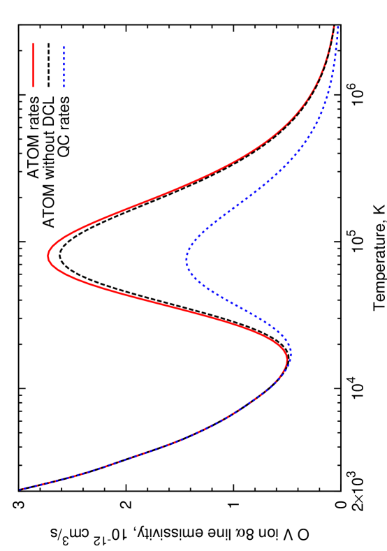
Figure 1: Temperature dependence of the O v 8$\alpha$ recombination line emissivity in the low-density limit. Lower curve correspond to DR rate computations using quasi-classical autoionization rates, upper curve – to the ATOM rates (for details see Appendix B.2), middle curve does not account for the process of line emission without recombination (DCL), described in Appendix B.6. At low temperatures the emissivity increase is determined by the radiative recombination, but the peak around $10^{5}$ K is arising due to the dielectronic recombination.

Emissivities of recombining $\@element[5+]{\mathrm{O}}$ optical and near-infrared recombination lines are given in Table 1 as functions of temperature in the low-density limit.

Approximate wavelengths of the brightest lines of all ions as functions of ionization stage are given in Table 2. They can be easily estimated using hydrogenic expressions for any recombination line arising in transition $n\to n^{\prime}$ between levels with $n^{\prime}>3$, $l>2$ as

$$\lambda(n\to n^{\prime})\approx\frac{0.091127}{Z^{2}}\,\left(\frac{1}{n^{\prime 2}}-\frac{1}{n^{2}}\right)^{-1}\,\mu{\rm m},$$ (3)

where $Z$ is the recombining ion charge.

Table 1: Wavelengths $\lambda$ and emissivities $\varepsilon$ of several O v optical and near-infrared recombination lines in the low-density limit.

		Emissivity $\varepsilon$, cm3/s, for electron temperature $T_{\rm e}$
Line	$\lambda$, $\mu$m	$1\cdot 10^{3}$ K	$3\cdot 10^{3}$ K	$1\cdot 10^{4}$ K	$3\cdot 10^{4}$ K
$5\alpha$	0.298	$9.4\cdot 10^{-12}$	$4.1\cdot 10^{-12}$	$3.5\cdot 10^{-12}$	$5.9\cdot 10^{-12}$
$6\alpha$	0.495	$7.6\cdot 10^{-12}$	$3.2\cdot 10^{-12}$	$1.2\cdot 10^{-12}$	$3.0\cdot 10^{-12}$
$7\alpha$	0.762	$6.3\cdot 10^{-12}$	$2.5\cdot 10^{-12}$	$8.8\cdot 10^{-13}$	$1.9\cdot 10^{-12}$
$8\alpha$	1.112	$5.2\cdot 10^{-12}$	$2.0\cdot 10^{-12}$	$6.7\cdot 10^{-13}$	$1.3\cdot 10^{-12}$
$9\alpha$	1.554	$4.4\cdot 10^{-12}$	$1.7\cdot 10^{-12}$	$5.2\cdot 10^{-13}$	$8.8\cdot 10^{-13}$
$10\alpha$	2.100	$3.7\cdot 10^{-12}$	$1.4\cdot 10^{-12}$	$4.1\cdot 10^{-13}$	$6.0\cdot 10^{-13}$
$11\alpha$	2.761	$3.2\cdot 10^{-12}$	$1.1\cdot 10^{-12}$	$3.3\cdot 10^{-13}$	$4.0\cdot 10^{-13}$
$12\alpha$	3.548	$2.7\cdot 10^{-12}$	$9.3\cdot 10^{-13}$	$2.6\cdot 10^{-13}$	$2.6\cdot 10^{-13}$

Table 2: Hydrogenic vacuum wavelengths, $\mu$m, of some optical and near-infrared recombination $\alpha$-lines for several ionization stages, denoted by the ion spectroscopic symbol after recombination.

Line	I	II	III	IV	V	VI
$4\alpha$	4.0501	1.0125	0.4500	0.2531	0.1620	0.1125
$5\alpha$	7.4558	1.8640	0.8284	0.4660	0.2982	0.2071
$6\alpha$	12.365	3.0913	1.3739	0.7728	0.4946	0.3435
$7\alpha$	19.052	4.7629	2.1168	1.1907	0.7621	0.5292
$8\alpha$	27.788	6.9471	3.0876	1.7368	1.1115	0.7719
$9\alpha$	38.849	9.7122	4.3165	2.4281	1.5540	1.0791
$10\alpha$	52.506	13.127	5.8340	3.2817	2.1003	1.4585
$11\alpha$	69.035	17.259	7.6705	4.3147	2.7614	1.9176
$12\alpha$	88.707	22.177	9.8563	5.5442	3.5483	2.4641

2.4 Resulting line fluxes

Fluxes $I(nl,n^{\prime}l^{\prime})$, erg/cm²/s, of the lines were finally computed by integrating along the line of sight

$$I(nl,n^{\prime}l^{\prime})=h\nu\frac{S}{4\pi R^{2}}\int\varepsilon\left(nl,n^{\prime}l^{\prime};T_{\rm e}(r)\right)n_{\rm e}(r)n_{+}(r){\rm d}r,$$ (4)

where $h\nu$ is the photon energy, $R$ is the distance from the observer to the emitting region and $S$ is the emitting region area.

The integral over distance in the plain-parallel approximation can be easily transformed into integral over temperature by substitution

$${\rm d}r=\frac{{\rm d}r}{{\rm d}t}\frac{{\rm d}t}{{\rm d}T}{\rm d}T=\upsilon_{\rm shock}\frac{3/2(n_{\rm t}+n_{\rm e})k_{B}}{n_{\rm t}n_{\rm e}\Lambda_{N}}{\rm d}T,$$

where $\upsilon_{\rm shock}$ is the shock front speed, $\Lambda_{N}$ is a cooling function and $n_{\rm t}$ is the total number density of all ions in plasma.

The parameters of this equation – cooling function, electron and ion densities as functions of temperature – were taken from the SD95 200 km/s shock model, described in more details in Section 3 below.

For purpose of qualitative analysis, we introduce below the oxygen differential emission measure per logarithmic temperature interval

$$\frac{{\rm d}\,E_{\rm O}}{{\rm d}\,(\log T_{\rm e})}=T_{\rm e}\,\frac{n_{\rm O}n_{\rm e}{\rm d}r}{{\rm d}T_{\rm e}},$$

where $n_{\rm O}$ is the total oxygen ion number density. It shows contribution of a given logarithmic temperature interval to the total emission measure, showing where most of the line emission originates. Using this notion, we can express the line flux from Eq. (4) as

$$I(nl,n^{\prime}l^{\prime})=h\nu\frac{S}{4\pi R^{2}}\int\varepsilon\left(nl,n^{\prime}l^{\prime};T_{\rm e}\right)\frac{{\rm d}\,E_{\rm O}}{{\rm d}\,\log T_{\rm e}}\;\frac{n_{+}}{n_{\rm O}}T_{\rm e}{\rm d}T_{\rm e}.$$

Here the fraction ${n_{+}}/{n_{\rm O}}$ is abundance of a given ionic species and is also dependent on temperature.

In our computation of the post-shock recombination line emission, we artificially stop integrating expression (4) when plasma temperature drops below 1000 K. This results in some, possibly significant, underestimate of the cooling region line fluxes arising from recombinations of $\@element[2+]{\mathrm{O}}$ ions. Though, as we show below, the O ii recombination lines from the photoionized region are expected to be much brighter.

It should be remembered that, e.g., O v recombination lines arise in the radiative cascade in the $\@element[4+]{\mathrm{O}}$ ion triggered by the recombination of $\@element[5+]{\mathrm{O}}$ ion, so the line fluxes are proportional to the ionic abundance of $\@element[5+]{\mathrm{O}}$, not $\@element[4+]{\mathrm{O}}$.

3 Astrophysical application: FMKs in Cassiopeia A

Figure 2: The plain-parallel SD95 model schematic structure. The drawing is not to scale. Arrow shows the shock wave direction. Optical lines are emitted from the photoionization front and the post-shock cooling region at temperatures of several tens of thousands Kelvin. Recombination lines arise in the cold photoionized region and the post-shock cooling region.

The SD95 model describes fast-moving knot emission as arising in the interaction of the oxygen-dominated dense cloud with the external shock wave, entering the cloud and propagating through it (see Figure 2). The heated region just after the shock front produces high flux of the ionizing radiation that results in appearance of two photoionized regions: before and after the shock front.

The plasma after the shock front passage is rapidly cooling and, at temperatures of $(1-5)\times 10^{4}$ K, emitting the lines observable in the visible and near-infrared spectra (Chevalier & Kirshner, 1978, 1979; Hurford & Fesen, 1996; Gerardy & Fesen, 2001). Thickness of this emitting layer is extremely small (about $10^{12}-10^{13}$ cm), but due to the high density of the cooling material at $T<10^{5}$ K it is able to produce bright emission lines of highly-ionized atomic species, such as [O iii]. This region also gives rise to the recombination line (RL) emission.

The SD95 model does not include the photoionized region after the shock front. Until now, even the presence of this region is disputed (Itoh, 1986) because, if present, it would produce too bright optical lines of neutral oxygen.

Between the photoionization front and the shock wave the plasma is predicted to be extremely cold ($T_{\rm e}<10^{3}$ K) and rather highly ionized (ionic abundances of $\@element[3+]{\mathrm{O}}$ and $\@element[2+]{\mathrm{O}}$ are about 60% and 30% in the SD95 200 km/s shock model). This cold ionized region, invisible in optical and X-ray bands, should be actively recombining and emitting bright recombination lines.

Resulting RL emission computed based on the SD95 200 km/s shock model is described separately in the following subsections for each of these two regions: after and before the shock front.

In this Section we provide results on the $l$-summed recombination line fluxes, whereas in the Section 4 we discuss in details the individual line spectral substructure, that separates in some cases the recombination lines into several components, thus diminishing the individual component fluxes up to factors of 2–4.

3.1 Cooling region after the shock front

It is useful to make order-of-magnitude estimates of some timescales in the post-shock rapidly cooling plasma at temperatures between several hundred and $3\times 10^{4}$ K, where the recombination line emission occurs (see below). As derived from SD95 model, the plasma cooling time is roughly equal to

$$\tau_{\rm cool}=\frac{3}{2}\frac{(n_{\rm t}+n_{\rm e})kT_{\rm e}}{n_{\rm t}n_{\rm e}\Lambda}\approx 2\times 10^{4}\;{\rm s}\;T_{4}^{1/2}\,n_{\rm t,5}^{-1},$$

where $T_{\rm e}=10^{4}T_{4}$ K and $n_{\rm t}=10^{5}n_{\rm t,5}$ cm^-3. It should be compared with the time needed to reach the collisional ionization equilibrium (CIE), that is in our caseis approximately equal to the recombination timescale $\tau_{\rm rec}$. For example, for ion $\@element[2+]{\mathrm{O}}$ and $\@element[6+]{\mathrm{O}}$ the recombination time is

$$\tau_{\rm rec}({\rm O}^{6+})=\left(n_{\rm e}q_{\rm RR,O^{6+}}(T_{\rm e})\right)^{-1}\approx 4.7\times 10^{5}\;{\rm s}\;T_{4}^{0.64}\,n_{\rm e,5}^{-1},$$

$$\tau_{\rm rec}({\rm O}^{2+})=\left(n_{\rm e}q_{\rm RR,O^{2+}}(T_{\rm e})\right)^{-1}\approx 4.9\times 10^{6}\;{\rm s}\;T_{4}^{0.64}\,n_{\rm e,5}^{-1},$$

where $n_{\rm e}=10^{5}n_{\rm e,5}$ cm^-3 and $q_{\rm RR,O^{2+}}$ is the total radiative recombination rate for this ion, taken from Pequignot et al. (1991). It is easy to see that the recombination timescale in this temperature interval is always longer than the cooling time for any abundant ion. Therefore the plasma is strongly overionized for its temperature, that results in high emissivities of the recombination lines.

The quantitative comparison of these timescales in the model is given on Figure 3, where ionization and recombination timescales for several ions are compared with the cooling time. At high temperatures the cooling timescale is longer than the ionization timescales and the material has enough time to converge to the CIE. At $T_{\rm e}<10^{6}$ K the cooling is much faster than the recombination down to temperatures of several hundred Kelvin and the high ionization state is stays “frozen” until very low temperatures are reached.

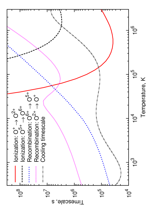
Figure 3: Oxygen ion $\@element[6+]{\mathrm{O}}$ and $\@element[2+]{\mathrm{O}}$ recombination and ionization timescales as compared to the plasma cooling time using the electron density dependence on temperature and the cooling function from the SD95 model with 200 km/s cloud shock speed.

Let us now compare the thermalization timescales and mean free paths to the quantities determined above. Following Spitzer (1956), the electron or ion self-collision timescale is equal to

$$\tau_{\rm c}=114\;{\rm s}\;\frac{A^{1/2}T_{4}^{3/2}}{n_{5}Z^{4}\ln\Lambda_{\rm C}},$$

where $A$ is the atomic weight (equal to 1/1836 for electrons), $Z$ is the particle charge, $n=10^{5}n_{5}$ cm^-3 is the particle concentration and $\Lambda_{\rm C}\approx 3.92\times 10^{7}\;n_{\rm e,5}^{-1/2}T_{4}^{3/2}$. In our case of the highly-charged plasma having $Z\gg 1$ the timescale of the ion-ion collisions is even shorter than for the electron-electron collisions.

Nevertheless, the mean free path even for electrons $\lambda_{\rm e}$ stays significantly below any other characteristic scale, including the typical temperature change length scale of more than $10^{12}$ cm:

$$\lambda_{\rm e}=\tau_{\rm c,e}\sqrt{3kT_{\rm e}/m_{e}}\approx 1\times 10^{7}\;{\rm cm}\;T_{4}^{2}\,n_{\rm e,5}^{-1}.$$

For illustration of the characteristic conditions after the passage of the shock front, on Figure 4 we show Li-like $\@element[5+]{\mathrm{O}}$ ion density as function of plasma temperature for this region. The figure demonstrates incredibly high abundance of this ion in relatively dense plasma with $T<3\times 10^{4}$ K after the shock front, much higher than in the CIE, where this ion exists only in a narrow temperature range $T_{\rm e}=(2-7)\times 10^{5}$ K (Mazzotta et al., 1998).

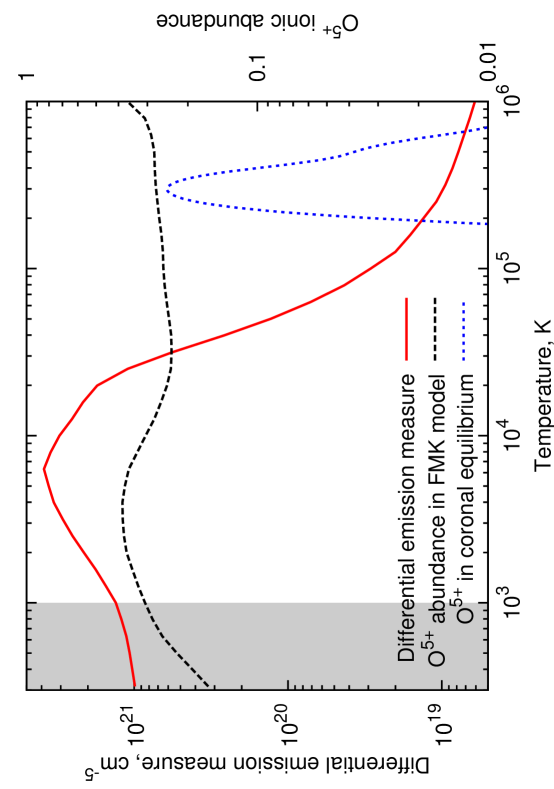
Figure 4: Differential oxygen emission measure per logarithmic temperature interval d$E_{\rm O}$/d$(\log T_{\rm e})$ in the post-shock cooling region of the SD95 FMK model. Ionic abundances $n$($\@element[5+]{\mathrm{O}}$)$/n({\rm O})$ of the $\@element[5+]{\mathrm{O}}$ ion in the FMK model and in the collisional ionization equilibrium in low-density plasmas (Mazzotta et al., 1998) are also shown. Temperature range not taken into account in our calculations is shaded.

On the same figure we present also the oxygen emission measure distribution over temperature d$(EM)/$d(log$T_{\rm e}$) in the SD95 model. This distribution together with the line emissivity dependence on temperature (e.g., Fig. 1) allows one to calculate the relative contributions to the total line flux from different temperature intervals (see Section 2.4 above).

Such line flux distributions for the prominent [O iii] line at 5007 Å and 8$\alpha$ lines of different oxygen ions are shown on Figure 5. Note that at low temperatures (below 4000 K), the [O iii] 5007 Å line emission is dominated by contribution from the recombinaiton cascades, not the collisional excitation. The cascade contribution to the post-shock intensity of this line reaches about 30%.

Because of high $\@element[6+]{\mathrm{O}}$ abundances at both low and high temperatures, the distribution of the O vi 8$\alpha$ line emission is much wider than that of the collisionally-excited optical [O iii] line and has 90% of its area within temperature range $5\times 10^{2}-1.5\times 10^{4}$ K. Note that the dielectronic recombination is contributing less than 20% to the resulting line intensity for any of oxygen ions in the discussed SD95 model.

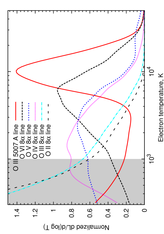
Figure 5: Differential luminosity distribution per logarithmic temperature interval according to the SD95 model for several spectral lines, including prominent 5007 Å [O iii] line and predicted O ii – O vi 8$\alpha$ lines. Curves are normalized so that the area enclosed under each of them equals one. Temperature range not taken into account in our calculations is shaded.

The O v and O vi lines are the brightest expected ones. Lines of O iii and O iv from this region are predicted to be dimmer by a factor of about three, and the O ii lines – by a factor of about ten.

On Figure 6 we show the predicted oxygen recombination line fluxes from the post-shock region of a model FMK. The brightest recombination lines around 1 $\mu$m are about 300 times less intense than the reddened [O iii] 5007 Å line. Expected flux values are given also in Table 3.

Table 3: Brightest recombination line $l$-summed emitted and reddened fluxes $I$ and $F$ from the post-shock cooling region computed following the SD95 model. The optical [O iii] 5007 Å line flux also given. The last column contains the flux part in the strongest unresolved line component $f_{\rm s}$. The wavelength $\lambda$ corresponds to the strongest line component.

Ion	Line	$\lambda$, $\mu$m	$I$, erg/cm2/s	$F$, erg/cm2/s	$f_{\rm s}$
O vi	7$\alpha$	0.5293	3.43$\times 10^{-16}$	3.15$\times 10^{-18}$	0.99
O vi	8$\alpha$	0.7720	1.83$\times 10^{-16}$	1.07$\times 10^{-17}$	0.99
O vi	9$\alpha$	1.0792	1.03$\times 10^{-16}$	2.14$\times 10^{-17}$	1.31∗
O vi	12$\beta$	1.3740	2.19$\times 10^{-17}$	7.42$\times 10^{-18}$	0.99
O vi	10$\alpha$	1.4586	6.08$\times 10^{-17}$	2.24$\times 10^{-17}$	1.00
O vi	13$\beta$	1.7189	1.49$\times 10^{-17}$	6.65$\times 10^{-18}$	1.00
O vi	11$\alpha$	1.9177	3.72$\times 10^{-17}$	1.83$\times 10^{-17}$	1.00
O vi	12$\alpha$	2.4642	2.35$\times 10^{-17}$	1.38$\times 10^{-17}$	1.00
O v	6$\alpha$	0.4943	4.07$\times 10^{-16}$	2.56$\times 10^{-18}$	0.62
O v	7$\alpha$	0.7618	1.99$\times 10^{-16}$	1.10$\times 10^{-17}$	0.81
O v	8$\alpha$	1.1114	1.06$\times 10^{-16}$	2.36$\times 10^{-17}$	0.89
O v	10$\beta$	1.1929	2.91$\times 10^{-17}$	7.66$\times 10^{-18}$	0.92
O v	9$\alpha$	1.5538	5.92$\times 10^{-17}$	2.36$\times 10^{-17}$	1.21∗
O v	12$\beta$	1.9784	1.24$\times 10^{-17}$	6.26$\times 10^{-18}$	0.96
O v	10$\alpha$	2.1002	3.47$\times 10^{-17}$	1.83$\times 10^{-17}$	0.94
O v	11$\alpha$	2.7613	2.12$\times 10^{-17}$	1.32$\times 10^{-17}$	0.97
O iv	7$\alpha$	1.1902	2.52$\times 10^{-17}$	6.62$\times 10^{-18}$	0.80
O iv	8$\alpha$	1.7363	1.32$\times 10^{-17}$	5.97$\times 10^{-18}$	0.74
O iii	5$\alpha$	0.8262	6.03$\times 10^{-17}$	4.57$\times 10^{-18}$	0.25
O iii	6$\alpha$	1.3727	2.65$\times 10^{-17}$	8.95$\times 10^{-18}$	0.25
O iii	7$\alpha$	2.1149	1.28$\times 10^{-17}$	6.78$\times 10^{-18}$	0.76
[O iii]		0.5007	9.32$\times 10^{-14}$	6.30$\times 10^{-16}$
[O iii]∗∗		0.5007	1.11$\times 10^{-12}$	7.52$\times 10^{-15}$
∗ Including 11$\beta$ line that is overlapping with 9$\alpha$
∗∗ Including the pre-shock photoionized region contribution

Note. Assumed cloud area is $1\times 10^{33}$ cm (size about 0$\aas@@fstack{\prime\prime}$6). Reddening was applied using Schild (1977) reddening curve and $E(B-V)=1.5$ (Hurford & Fesen, 1996). The brightest knots are a factor of 3–10 more intense in the [O iii] 5007 Å line than the values given in the table. The $f_{\rm s}$ values were determined from simulated spectra having 200 km/s Doppler line width at the half maximum level (FWHM), that is equal to the optical line widths observed in the Cas A knots (van den Bergh, 1971); see also Section 4.

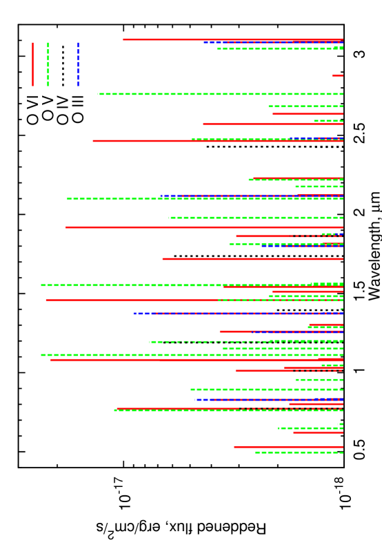
Figure 6: Reddened recombination line $l$-summed fluxes $F$ from the post-shock cooling region. Details are as in note to Table 3. Here the lines are represented as “infinitely thin”; their fine structure is discussed in Section 4.

3.2 Cold photoionized region

The ions in the photoionized region before the shock front are rapidly recombining because of their low temperature. This results in rather bright recombination lines, with fluxes proportional to the distance $d$ between the ionization front and the shock wave.

The plain-parallel SD95 model does not determine this distance. Assumption of small optical depth of material between the shock wave and the ionization front results in restriction of $d<10^{17}$ cm for relevant cloud models for preshock ion number density of 100 cm^-3 (illustrated on the Figure 12 of SD95). Below we take conservatively $d=10^{16}$ cm, keeping in mind that the line fluxes scale linearly with it.

The cloud model also do not determine exact temperature in the photoionized region. We take $T_{\rm e}=1\times 10^{3}$ K as a reference value, but Dopita et al. (1984) mention that it may be as low as 100 K. If the real temperature in the region is less than our assumed value, recombination line emissivities are respectively higher (see Section 5.1 below for quantitative dependences).

Predicted oxygen line fluxes for the SD95 model OP200 with shock speed of 200 km/s and total preshock ion number density 100 cm^-3 are shown on Figure 7 and given in Table 4. It is seen that even with our quite conservative assumptions resulting line fluxes are still somewhat stronger than from the shock front. Indeed, the predicted line brightest components are on the level of almost half a percent of the [O iii] 5007 Å line.

Table 4: Brightest recombination line $l$-summed emitted and reddened fluxes $I$ and $F$ from the photoionized region before the shock front. computed following the SD95 model. Details are as in note to Table 3. Photoionized region thickness is $10^{16}$ cm. The last column contains the flux part in the strongest unresolved line component $f_{\rm s}$ for FWHM of 200 km/s (see Note to Table 3). The wavelength $\lambda$ corresponds to the strongest line component.

Ion	Line	$\lambda$, $\mu$m	$I$, erg/cm2/s	$F$, erg/cm2/s	$f_{\rm s}$
O iii	5$\alpha$	0.8262	4.13$\times 10^{-16}$	3.26$\times 10^{-17}$	0.26
O iii	6$\beta$	0.8327	1.05$\times 10^{-16}$	8.48$\times 10^{-18}$	0.31
O iii	7$\beta$	1.2552	6.09$\times 10^{-17}$	1.77$\times 10^{-17}$	0.73
O iii	6$\alpha$	1.3727	1.95$\times 10^{-16}$	6.61$\times 10^{-17}$	0.27
O iii	8$\beta$	1.7998	3.69$\times 10^{-17}$	1.72$\times 10^{-17}$	0.86
O iii	7$\alpha$	2.1149	1.00$\times 10^{-16}$	5.32$\times 10^{-17}$	0.82
O iii	9$\beta$	2.4804	2.32$\times 10^{-17}$	1.36$\times 10^{-17}$	1.32∗
O iii	8$\alpha$	3.0871	5.50$\times 10^{-17}$	3.59$\times 10^{-17}$	0.91
O ii	5$\alpha$	1.8645	4.03$\times 10^{-17}$	1.94$\times 10^{-17}$	0.24
O ii	6$\alpha$	3.0922	1.90$\times 10^{-17}$	1.24$\times 10^{-17}$	0.59
∗ Including 10$\gamma$ line that is overlapping with 9$\beta$

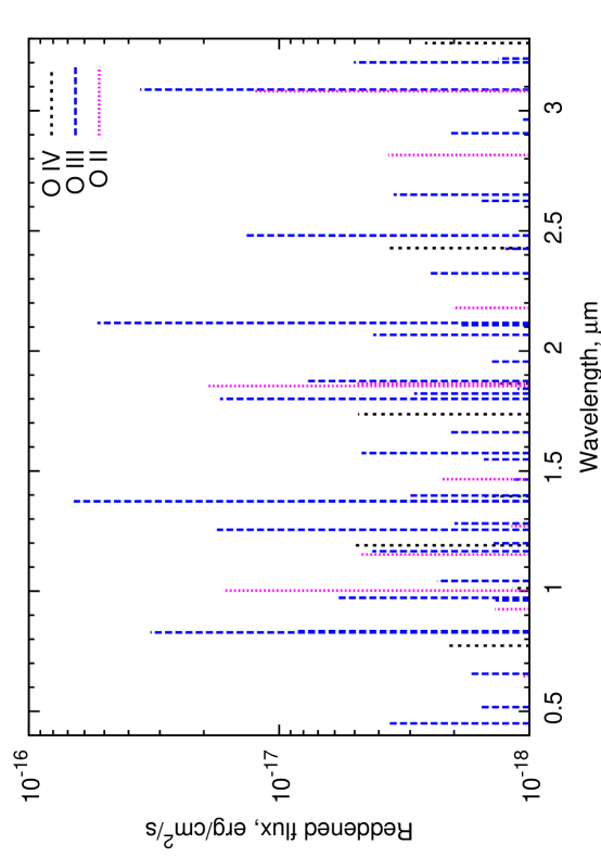
Figure 7: Recombination line $l$-summed reddened fluxes expected from the photoionized region before the shock front computed following the SD95 ionization front model. Details are as in note to Table 3. Photoionized region thickness is $10^{16}$ cm.

If they would be just a factor of several stronger, the lines would have been detected in spectroscopic observations of the fast-moving knots (see discussion on existing observation limits in Section 3.4 below).

Our estimate of the observational limit on the O iii 5$\alpha$ recombination line flux at 0.83 $\mu$m based on the data by Hurford & Fesen (1996) of $0.005\times F$(5007 Å) may be transformed into a joint constraint on the thickness of the photoionized region $d$, its temperature $T_{\rm e}$ and total ion density $n_{\rm t}$:

$$\left(\frac{n_{\rm t}}{100\,{\rm cm^{-3}}}\right)^{2}\,\left(\frac{10^{3}\,{\rm K}}{T_{\rm e}}\right)\,\left(\frac{d}{10^{16}\,{\rm cm}}\right)<7,$$

assuming $E(B-V)=1.5$ and $\@element[3+]{\mathrm{O}}$ ionic abundance after the ionization front of 0.6.

On this example it is easy to see that detection of the lines or even tight upper limits will allow to perform detailed observational tests of the SD95 and other FMK models.

3.3 Separating pre- and post-shock spectral lines

Observationally, the lines formed in the regions before and after the shock wave will be distinguishable because of two effects. Firstly, the lines arising in the photoionized region yet dynamically undisturbed by the shock wave should be intrinsically very narrow, but the lines arising in the post-shock region are expected to be Doppler-broadened by turbulence.

Secondly, the spectral lines arising in the post-shock region should be shifted with respect to the pre-shock lines. The relative Doppler shift between these two line families appears due to motion of the post-shock gas relative to the initial knot speed induced by the shock wave. In the strong-shock limit this velocity difference equals $3/4\,\upsilon_{\rm shock}$ for specific heat ratio $\gamma=5/3$ (Zel’dovich & Raizer, 1967), i.e. up to 150 km/s in the SD95 model, but the relative Doppler shift will also depend on the angle between the shock front and the direction towards observer.

Both collisionally-excited and recombination lines should display these features, but for the former group such differences should be easier to detect because of higher line intensities.

The observations with higher spectral resolution ($\lambda/\Delta\lambda\la 20\,000$) could also result in detection of several narrow components forming a line. They could arise from the individual vortice or velocity component emission, if there is only one or a few of them dominating the plasma motions after the shock, like observed in laser experiments simulating cloud-shock interaction in supernova remnants (Klein et al., 2003). The resulting spectral line profile might be quite complicated (e.g., Inogamov & Sunyaev (2003)), but such observations will provide data on the post-shock dynamics of the fast-moving knot that is presently poorly constrained from observations.

3.4 Existing observational limits

As it is seen from Figures 6 and 7, the brightest recombination lines are expected to lie in the wavelength range between 0.7 and 3 $\mu$m. Several detailed spectroscopic investigations have already been performed in this range and could have found these lines, provided that they had low enough detection limits. Below we discuss such existing optical and near-infrared limits on the line fluxes and compare them with the SD95 model predictions.

Optical spectra of fast-moving knots with wide spectral coverage were obtained, e.g., by Chevalier & Kirshner (1979) and Hurford & Fesen (1996). According to the authors, the detection limits around 0.75–0.85 $\mu$m are about 300 times less than the [O iii] 5007 Å line flux for the brightest observed features.

Our results give flux ratios of the reddened 5007 Å line to the brightest components of the O vi 8$\alpha$, O v 7$\alpha$ and O iii 5$\alpha$ lines of about 300–500 (see Figures 6 and 7 and Tables 3 and 4). These values show that the model is on the boundary of consistency with the observational results. They also imply that the oxygen recombination line detection should be possible, provided that the physics in the post-shock and pre-shock regions corresponds to the one described by the SD95 model.

Recently, near-infrared (0.95–2.5 $\mu$m) spectra of Cas A fast-moving knots, obtained at the 2.4 m Hiltner telescope, were published by Gerardy & Fesen (2001). It is more difficult to compare their detection limits with our predictions, as there is only one oxygen O i line blend present around 1.129 $\mu$m. It arises in transitions between excited states of neutral oxygen and is also blended with [S i] line. If we assume that the overlapping [S i] line emission is negligible, our estimate of the observational detection limit corresponds to about 1/100 of the reddened optical [O iii] line flux. This value is a factor of several higher than the predicted fluxes of the O vi 9$\alpha$, O v 8$\alpha$ and O iii 6$\alpha$ lines, also showing feasibility of the line detection.

4 Individual line substructure

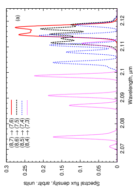
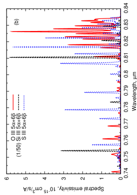
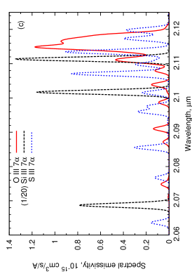
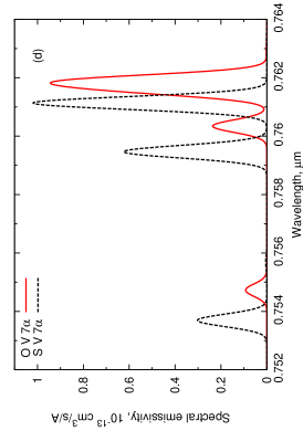
Figure 8: Fine structure of recombination lines. Line Doppler width at half maximum of 200 km/s is assumed. (a): O iii $7\alpha$ line $(8,l)\to(7,l-1)$ component structure for $l\geq 4$. Sum of all components is set to be equal for each $l$. Emissivities of the $(8,l)\to(7,l+1)$ components are much weaker and structure of resulting lines is not shown. (b),(c): Spectral emissivity d$\varepsilon/$d$\lambda$, cm³/s/Å of the simulated O iii, Si iii and S iii $5\alpha+6\beta$ and $7\alpha$ line structure for low-density case and temperature $T_{\rm e}=2\times 10^{4}$ K. Note that Si iii lines have been scaled down to fit in the same scale. (d): Spectral emissivity for the simulated O v and S v $7\alpha$ line structure in the same conditions. Absence of $K$-splitting results in much simpler profiles.

In the non-relativistic hydrogenic approximation, level energies depend only on the ion charge and the principal quantum number $n$ of the level. Though, this approximation is not fully applicable for the description of the spectral lines corresponding to transitions between the levels with $n\approx 10$, as other effects start playing a role. They arise due to energy level shifts, described in Appendix B.4, resulting in the “fine” structure appearing in the spectral lines. As a result, these effects help to distinguish lines of different elements having equal ionization stages and initial and final $n$’s.

We calculated the line $l$– and $K$–substructure following the method outlined in Appendix B.5 ($K$ is the quantum number used to characterize additional interaction of the highly-excited electron orbital momentum with the total angular momentum of other electrons, present in O ii, O iii, S ii and S iii lines). The results are shown on Figure 8 for several most interesting cases, assuming recombination lines having widths around 200 km/s (full width at half maximum level, FWHM), of the same order as the observed widths of forbidden optical lines (van den Bergh, 1971).

It is easily seen that high-$l$ levels have both smaller quantum defects and smaller $K$-splitting. Complicated line structure in case of presence of the $K$-splitting results in weaker individual line fluxes making them more difficult to detect.

One should also keep in mind that spectral lines arising in transitions between lower-$n$ levels have higher $K$- and $l$-splittings. Therefore the line components have larger separations and the amount of individual components increase even more with each of them being respectivly less intense. As a bottomline, the near-infrared lines are more promising for the first detection than the optical ones, as they have less substructure (compare panels (b) and (c) on Figure 8).

The substructure of the 6$\alpha$ recombination lines of Mg i, Al i and Si i have been observed in solar spectra near 12 $\mu$m and explained using similar, although somewhat more elaborate, theoretical description (Brault & Noyes, 1983; Chang & Noyes, 1983; Chang, 1984). We have used these observations as the test cases for our line substructure computation code.

In Tables 5–15, available as an electronic supplement at the CDS, we give O ii – O vi, S ii – S v, Si ii and Si iii recombination line component vacuum wavelengths, emissivities and relative intensities in the $(nlK)\to(n^{\prime}l^{\prime}K^{\prime})$ resolution for several temperatures (lg$(T_{\rm e},{\rm K})=$3.0, 3.5, 4.0, 4.5 and 5.0) in the low-density limit. First seven columns characterize the quantum numbers of the transition (total recombining ion electronic angular momentum $J_{\rm c}$ and highly-excited electron quantum numbers before and after the transition $n$, $l$, $K$, $n^{\prime}$, $l^{\prime}$, $K^{\prime}$), Column 8 gives the line component wavelength in microns, next columns in pairs state line component emissivity in cm³/s and intensity ratio of this component with respect to the $K$- and $l$-summed emissivity $\varepsilon(J_{\rm c},nlK,n^{\prime}l^{\prime}K^{\prime})/\varepsilon(n,n^{\prime})$. Only the lines most likely to be detected are given in these tables, selected by the following parameters – only $\alpha$, $\beta$ and $\gamma$ lines having wavelengths between 0.3 and 5.0 $\mu$m.

Tables 16–23, also available at the CDS, contain similar information on predicted oxygen line component fluxes in the SD95 200 km/s shock model. The fluxes from the cooling and photoionized regions are given separately in Tables 16–20 (for O ii – O vi) and 21–23 (for O ii – O iv), respectively. First eight columns again contain the quantum numbers characterizing the transition and the line wavelength, Column 9 lists line component flux in erg/cm²/s, Column 10 contains intensity ratio of this component with respect to the $K$- and $l$-summed emissivity.

As discussed in Appendix B.4, the input atomic data are precise to about 10% and we cannot expect better precision of the resulting line wavelength differences from the hydrogenic values.

Sample region from the total resulting model spectrum is shown on Figure 9. It shows variety of the spectral shapes as well as illustrates the diminishing of the peak intensity due to $K$-splitting for O iii lines.

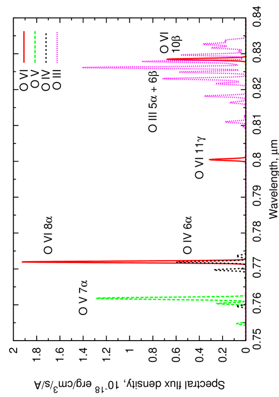
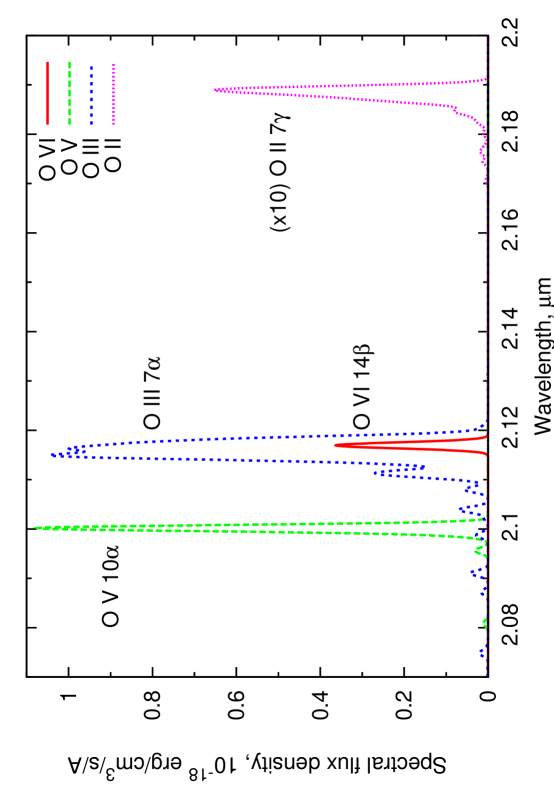
Figure 9: Model spectra near 0.8 and 2.1 $\mu$m containing recombination lines of O ii–O vi computed based on the SD95 200 km/s shock model. Contributions of cooling and photoionized regions are summed up. It is seen that at longer wavelengths the substructure is less influencing the line profiles. Note that O ii $7\gamma$ line intensity is multiplied by 10 for illustration purposes. Line FWHM of 200 km/s is assumed.

The line substructure change with density and temperature because of changes in the relative populations of the $l$-states. At low temperatures the main population mechanism is the radiative recombination, which is populating high-$l$ levels relatively efficient. When the electron density increases, $l$-redistribution modifies high-$l$ populations for $n$ greater than about 20, but for $n<15$ the changes are generally smaller.

At higher temperatures, DR populates relatively lower $l$ states having higher quantum defects and low probabilities of $\alpha$-line emission. Therefore a recombination line is split into many components and its emissivity is relatively low. In this case, $l$-redistribution mostly shift the recombined electrons to higher-$l$ states, simplifying the line profile and significantly increasing its emissivity.

On Figure 10 we show the change of the O iii $7\alpha$ line fine structure with temperature and density, illustrating the described effects.

Another effect arising at low temperatures and electron densities – lower populations of excited $J_{\rm c}$ core states. For O ii, O iii, S ii and S iii lines this results in damping of the $K$-splitting, as it arises only from recombination of excited ions. All the flux from $(nlK)\to(n^{\prime}l^{\prime}K^{\prime})$ components in this case will be redistributed into the central $(nl)\to(n^{\prime}l^{\prime})$ components and only the $l$-splitting will remain.

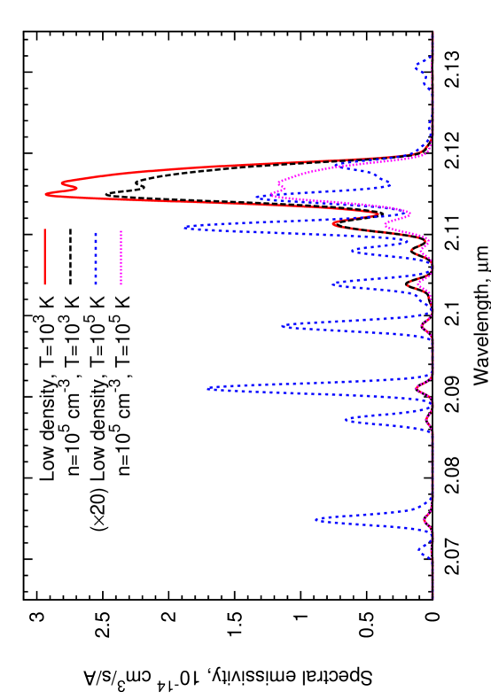
Figure 10: Variation of the fine structure of the O iii $7\alpha$ line at 2.1 $\mu$m with temperature and density. Line FWHM of 200 km/s is assumed. Note that the low-density curve for $T_{\rm e}=10^{5}$ K is multiplied by 20 to be visible on this scale.

5 Plasma diagnostics using recombination lines

5.1 Temperature diagnostics

Line emissivity dependence on temperature is shown for several bright optical and near-infrared oxygen recombination lines in the low-density limit on Figure 11. Corresponding line wavelengths are given in Table 2 above. This figure allows to compute the recombination line fluxes for other models of the multi-temperature plasma with emission measure distribution different from the discussed SD95 model.

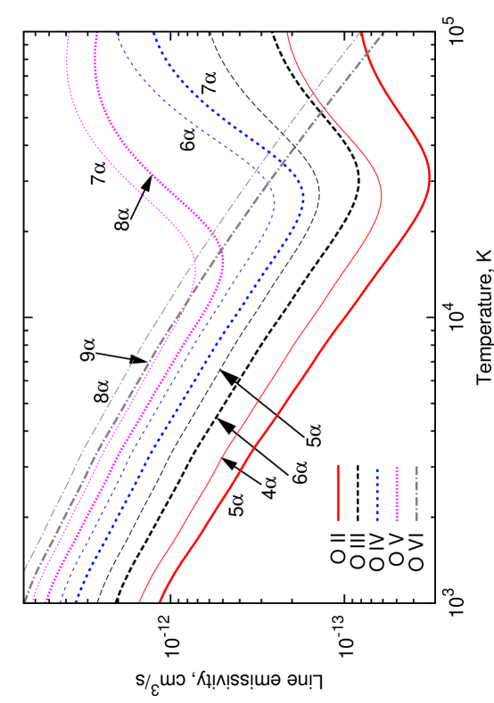
Figure 11: Low-density $l$-summed emissivities of oxygen ion optical and near-infrared recombination lines. Different colors represent different ions, plotted line thickness increase with the spectral line wavelength.

The curves on Figure 11 has two distinct regions. At low temperatures the emissivity is determined by the radiative recombination and changes smoothly from ion to ion. At temperatures higher than several tens of thousands Kelvin the dielectronic recombination starts to dominate the recombination rates (except for the O vi lines due to absence at low temperatures of dielectronic recombination channels in He-like ion $\@element[6+]{\mathrm{O}}$) and line emissivities of different ions start being determined by the lowest excited states of the recombining ion, as described in Appendix B.2. The temperature of the strong emissivity rise is proportional to the typical energy of such excited states. Amplitude of the rise is proportional to the lowest excited state decay rate.

For the discussed SD95 200 km/s shock model the high-temperature region where the DR dominates is important only for O v lines, but it is easy to imagine other ionic abundance distributions where it will affect also ions in lower ionization stages.

Dependence of individual O v recombination $\alpha$-line ratios on temperature is shown on Figure 12. Again, the two distinct regions are seen at low and high temperatures corresponding to RR- and DR-dominated recombination.

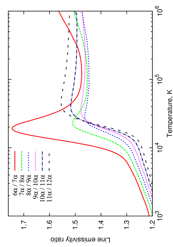
Figure 12: Low-density $l$-summed O v recombination line emissivity ratios as functions of electron temperature.

It is easy to notice that in the intermediate temperatures, the lines corresponding to transitions at lowest $n$’s become relatively brighter. Reason for such dependence, especially clearly visible on the $6\alpha/7\alpha$ line ratio, is the following. As follows from Appendix B.2, at low temperatures the dielectronic recombination rate is damped by the factor $\exp\left(-{\mathcal{E}}/{kT_{\rm e}}\right)$. For the low $n$-levels the doubly excited state energy $\mathcal{E}$ may be significantly lower than the core excitation energy and at low temperatures this makes a difference and the dielectronic recombination populates mostly low-$n$ levels, increasing emissivities of low-$n$ recombination lines.

The described effect is most pronounced for recombination lines of O v, Si iii and S v, although in all cases the most temperature-sensitive line – the $\alpha$-line formed by the transition from the lowest level, onto which DR is possible – is situated around 2000–3000 Å. Though, as can be seen from Figure 12, also the next line situated for these ions around 4500–5000 Å, can also be a useful diagnostical tool, being relatively much brighter in a narrow temperature interval.

5.2 Recombination lines as density diagnostics

Recombination line flux ratios allow in principle to determine also density of the emitting region, as their dependences on density and temperature differently affect the relative line fluxes.

As an example, on Figure 13 we plot the O v $7\alpha$ line emissivity as function of the electron density for different temperatures between $10^{3}$ and $10^{5}$ K. For better representation, emissivity ratios to their low-density values are shown. Clearly, the density dependences are weak and can probably be neglected in the first stage of the qualitative analysis, especially at low temperatures.

Two distinct regions are seen once again. At low temperatures where only radiative recombination determines the level populations, emissivities decrease with density, but at higher temperatures they increase. The difference is explained by different initial populations of the levels.

Dielectronic recombination predominantly populates states with $l\la 10$ (see, e.g., Appendix B.2). Collisions in this case mostly transfer recombined electrons to higher $l$’s, increasing the probability of $\Delta n=1$ transitions and, therefore, $\alpha$-line emissivities.

Radiative recombination, especially at low temperatures, populates high-$l$ states much more efficiently. In this case, populations of low-$l$ levels relatively increase as a result of the $l$-changing collisions, and recombination line emissivities somewhat decrease.

On Figure 14 we show the O v recombination line emissivities relative to their low-density values as functions of electron density at temperature 30 000 K. Lines arising in transitions between higher levels increase relatively more, but in absolute terms the increase in emissivity is approximately constant, determined by the $l$-redistribution on the high-$n$ levels.

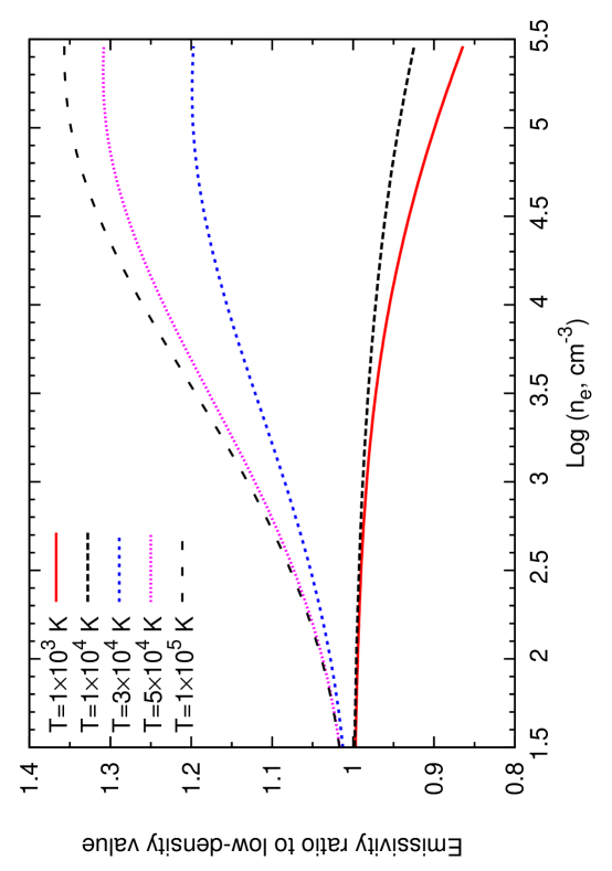
Figure 13: Dependence of O v $7\alpha$ line emissivity on electron density for different electron temperatures $T_{\rm e}$. Values are normalized to the low-density emissivity.

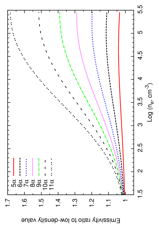
Figure 14: Increase of O v $\alpha$-line emissivities with electron density at temperature $T_{\rm e}=3\times 10^{4}$ K.

5.3 Recombination lines of other elements

Our previous analysis mainly concerned the oxygen recombination line emission, as the SD95 model allows making quantitative predictions about their fluxes and line ratios to the observed collisionally-excited lines. For other elements, no model results for ionic abundance distribution are available. Thus to predict their line fluxes it is necessary to solve a separate problem of non-equilibrium plasma cooling and recombination after the shock front for dense clouds of different compositions. Such analysis is outside the scope of this paper.

Nevertheless, it seems valuable to provide data on the recombination line emissivities as functions of temperature for the most typical elements. Then, from measured line ratios, it will be possible to reconstruct characteristic conditions in the emitting regions. As two most typical examples for elements composing FMKs in Cas A, we concentrate on the recombination lines of silicon and sulphur. Approximate wavelengths of their recombination lines are given in Table 2 above.

Figure 15 presents low-density emissivities of brightest optical and near-infrared recombination lines of silicon and sulphur ions, expected to exist in the fast-moving knots. Note that Si iv and S vi lines are much weaker than of the other ions at $T_{\rm e}>10^{4}$ K due to weakness of dielectronic recombination channels at these temperatures. Note also that the line emissivities in Si ii and Si iii ions start to increase sharply already at about 12 000 K.

Thus these ions are the most sensitive tracers of plasma at temperatures between 15 000 and 30 000 K, when emissivities of O and S ions are yet relatively weak. This is also seen on Figure 8(b,c) above, where the emissivities of the lines of Si iii are a factor of 20-50 higher than that of O iii and S iii in the same conditions.

Resembling the case of oxygen recombination lines, the density dependences are not pronounced.

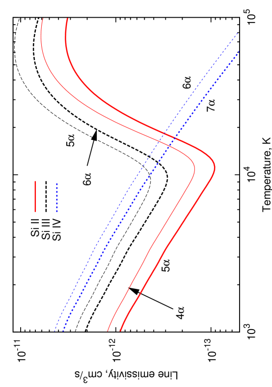
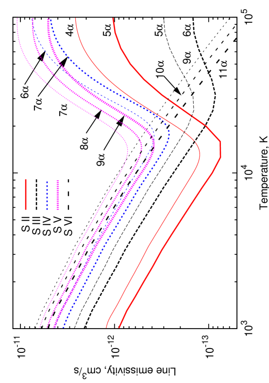
Figure 15: Low-density $l$-summed emissivities of several optical and near-infrared silicon and sulphur recombination lines. Different colors represent different ions, plotted line thickness increase with spectral line wavelength.

5.4 Ratios to collisionally-excited lines

Comparison of metal recombination line fluxes with the “traditional” collisionally-excited lines may also be a useful tool for plasma diagnostics.

As these two types of lines have different origin, their emissivity dependences on temperature and density are rather different. For example, collisionally-excited line emissivities exponentially drop at temperatures below about $h\nu/k$, as thermal electron energies are not sufficient to excite the ion electronic transition. In contrast, recombination line emissivities at low temperatures increase with the temperature decreasing.

Also a useful property is that, even in the case when the recombination lines are not detected at all, from the limits on the ratios to the collisional lines it is possible to put constraints on the plasma parameters.

On the Figure 16 we give ratios to several brightest collisionally-excited optical lines. The exponential increase of ratios at low temperatures is clearly seen. Collisional line emissivities have been computed using Chianti atomic database (Dere et al., 1997; Landi et al., 2006)

Ratios to the fine-structure far-infrared line emissivities are given on Figure 17. As the Chianti database does not allow to compute line emissivities down to 100 K, we computed them by extrapolating fine-structure transition electronic excitation collision strengths to low temperatures by a constant, that should be reliable to within a factor of two. The collision strength values were adopted from calculations by Lennon & Burke (1994); Blum & Pradhan (1992); Tayal & Gupta (1999); Tayal (2000, 2006).

We note that observations of the far-infrared lines in the spectral range from 10 to 100 $\mu$m are impossible from the ground. But even from space, observations of these very intense lines cannot be performed with angular resolution sufficient for resolving individual knots. They can result only in signal integrated over many individual emitting objects.

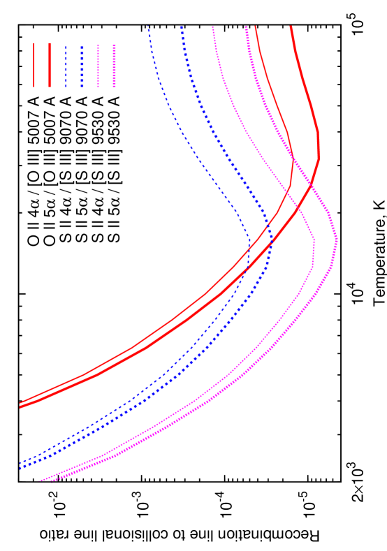
Figure 16: Low-density emissivity ratios of recombination lines to several brightest optical collisionally-excited lines.

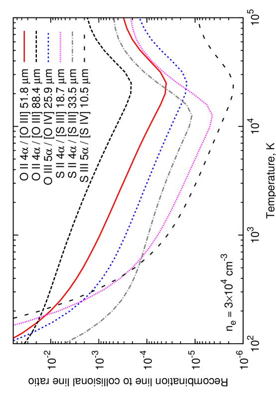
Figure 17: Emissivity ratios of recombination lines to several far-infrared collisionally-excited lines. Upper and lower panels show emissivity ratios in the low-density limit applicable for the cold photoionized region (except for the 88.4 $\mu$m line) and the case of $n_{\rm e}=3\times 10^{4}$ cm^-3 typical for the cooling region after the shock front.

Density dependences of recombination and collisionally-excited lines are also different. Forbidden line emissivity starts decreasing as $1/n_{\rm e}$ at some critical density, whereas the recombination line emissivities may both decrease and increase depending on the plasma temperature (see above).

The best density indicators for relatively low temperatures and densities in the fast-moving knots are obviously ratios of different optical and near-infrared line to the far-infrared lines that have critical densities of the order of $100-10^{4}$ cm^-3. In the accompanying paper (Docenko & Sunyaev, to be submitted), we present such analysis based on existing experimental data and compare the results with our predictions based on the SD95 model.

6 Conclusions

We have offered and developed in detail a new method of rapidly recombining plasma diagnostics based on measurements of optical and near-infrared recombination lines of multiply-ionized metal atoms.

As a promising example, we have applied our method to the SD95 theoretical model of fast-moving knots in Cassiopeia A supernova remnant and computed expected oxygen line fluxes from a single FMK of average size and resulting recombination line ratios. It turned out that both cold photoionized region before the shock front and rapidly cooling region immediately after the shock front produce oxygen recombination lines strong enough to be observed on modern optical telescopes in the wavelength range between 0.5 and 3 $\mu$m.

At shorter wavelengths, two reasons hamper the line observations: high absorption in the interstellar medium on the way from Cas A and the line splitting into widely separated multiple components with consequently lower intensities in each of them. The lines $n\alpha$ corresponding to transitions between $n\geq 6$ levels are the most promising, as they are not so strongly split and have 50-90% of intensity in one or a few narrow components.

The precision of our RL flux estimates from the Cas A is not expected to be better than a factor of several, as inconsistencies of similar magnitude are observed between the SD95 model predictions and far-infrared oxygen line observations (Docenko & Sunyaev, to be submitted).

Nevertheless, when detected, the recombination lines will allow to determine the details of the photoionization and rapid cooling processes in the FMKs from the line intensities, intensity ratios to each other and to forbidden collisionally-excited lines and from the recombination line fine structure measurements. The measurements of the line structure demand higher signal-to-noise ratios that can nevertheless be achieved on modern telescopes in a reasonable integration time of few hours.

One very interesting result is that the predicted O v and O vi recombination lines, being brightest in the cooling region recombination line spectra, arise in the temperature range significantly below $10^{5}$ K, where there is essentially no O⁵⁺ and O⁶⁺ ions in the collisional ionization equilibrium conditions.

It would be also very interesting to observe the recombination lines from the knots consisting mostly of silicon and sulphur. Existence of high-temperature shock-heated plasma having such chemical composition have been proved by X-ray spectral observations (e.g., Hughes et al. (2000); Hwang et al. (2004)), but detailed theoretical predictions of cooling and ionization structure of such clouds have not been developed yet.

One of the purposes of this article is to attract attention to the metal recombination lines radiated by plasma being far out of the collisional ionization equilibrium and having highly-charged ions at low temperatures. Besides the supernova remnants, such plasma producing detectable metal recombination lines may exist in planetary nebulae, as well as near quasars and active galactic nuclei.

Appendix A Determination of the upper cutoff $n_{\rm max}$

Traditionally, the highly-excited level populations are characterized by the so-called departure coefficients $b_{nl}$, defined as the ratio of actual level population $N_{nl}$ to its thermodynamic equilibrium value $N_{nl}^{*}$. With $n$ increasing, at levels $n>n_{1}$ the collisional $l$-redistribution processes establish equilibrium population over $l$’s, i.e., $b_{n}=b_{nl}$. The value of $n_{1}$ depends on the ion, as well as on electron temperature and number density.

For higher $n$’s, rates of collisional transitions involving $n$ change start rapidly increasing and from some $n>n_{2}$ determine the highly-excited level populations. Thus the $b_{n}$ curve, itself defined only at $n>n_{1}$, has two distinct ranges as a function of $n$: below $n=n_{2}$ it is determined by recombination and radiative processes and above it rapidly tends to unity because of the processes relating different $n$ level populations with each other and with the continuum: collisional $n$-redistribution, three-body recombination and collisional ionization. As an example relevant for our study, $b_{n}$’s of Li-like ion $\@element[5+]{\mathrm{O}}$ at temperatures 1000 and 20 000 K and electron density 50 000 cm^-3 are shown on Figure 18, assuming $b_{n}=b_{nl}$.

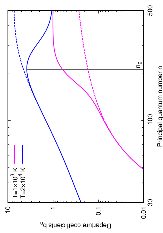
Figure 18: Departure coefficients $b_{n}$ of recombining $\@element[5+]{\mathrm{O}}$ ions computed accounting for all processes (solid lines) and neglecting collisional $n$-redistribution, three-body recombination and collisional ionization (dashed lines) at electron temperatures $T_{\rm e}=1\times 10^{3}$ K and $2\times 10^{4}$ K and density $n_{\rm e}=5\times 10^{4}$ cm^-3. At higher temperature dielectronic recombination dominates and significantly increases the level populations.

On this figure, we also show the departure coefficients, computed accounting only for radiative $n\to n^{\prime}$ transitions. It is seen that such approximation results in population computation errors at levels higher than about $n_{2}$.

Let us now show that the electrons that recombined to levels $n>n_{2}$ are contributing relatively weakly to the total recombination and it is safe to introduce an upper cutoff $n_{\rm max}$, neglecting population of higher levels. Two cases – $b_{n_{2}}>1$ and $b_{n_{2}}<1$ – should be discussed separately here.

In case of $b_{n_{2}}>1$ not introducing such cutoff and neglecting $n\to n^{\prime}$ collisions may result in some cases in significant overestimate of the recombination rate – up to a factor of several. The easiest estimate of the cutoff position is the level where the total recombination rate onto $n<n_{\rm max}$ computed without accounting for $n\to n^{\prime}$ transitions equals to the true total recombination rate. It is easy to understand that in this case $n_{\rm max}\approx n_{2}$, as illustrated in the lower panel of Figure 19.

In case of $b_{n_{2}}<1$ the rates obtained neglecting collisional transitions between high levels will always underestimate true recombination rates. Though for temperatures above about $10^{3}$ K taking upper cutoff value approximately equal to $n_{2}$ does not result in error more than about 20% for relevant ions, as illustrated on the upper panel of the Figure 19. Lower cutoff values will result in more significant underestimates of the total recombination rate and the line emissivities.

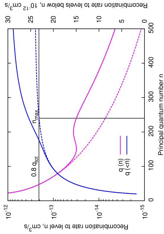
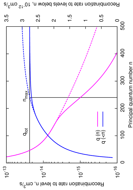
Figure 19: Recombination rates $q$ of $\@element[5+]{\mathrm{O}}$ for $n_{\rm e}=5\times 10^{4}$ cm^-3 and $T_{\rm e}=1\times 10^{3}$ K (upper panel) and $2\times 10^{4}$ K (lower panel). Meaning of solid and dashed lines is as on Figure 18. Plot shows both rates for a given $n$ (magenta curves) and cumulative rates for all levels below $n$ (blue curves). Vertical line show upper cutoff $n_{\rm max}$ used for this ion in our calculations.

In case of lower densities, when $n_{2}$ is very high, another natural limit $n_{\rm max}\approx(100-200)$ arises from general dependence of the DR rate on the principal quantum number, see, e.g., Sobelman et al. (1981).

Appendix B Atomic physics for level population computations

B.1 Radiative recombination

There are two major recombination processes populating high-$n$ states in low-density plasmas: radiative and dielectronic recombination (RR and DR, respectively). In the radiative recombination process, a free electron is directly recombining to a bound state $(nl)$. A photon is simultaneously emitted, carrying away the released energy.

The radiative recombination level-specific cross sections $\sigma_{\rm RR}$ were computed from hydrogenic photoionization cross sections $\sigma_{\rm PI}$ by applying the detailed balance relation:

$$\sigma_{\rm RR}(\mathcal{E}\to nl)=\frac{\alpha^{2}Z^{2}}{2}\,\frac{2l+1}{n^{2}}\,\frac{\nu^{2}}{\nu_{n}(\nu-\nu_{n})}\,\sigma_{\rm PI}(nl\to\mathcal{E}),$$ (5)

where $\mathcal{E}$ is the electron energy prior to recombination, $h\nu_{n}={\rm Ry}\,Z^{2}/n^{2}$ is the level binding energy, $h\nu=\mathcal{E}+h\nu_{n}$ is the energy of emitted photon, $Z$ is the recombining ion charge and $\alpha$ is the fine-structure constant. The photoionization cross sections $\sigma_{\rm PI}$ were calculated by the computer program of Storey & Hummer (1991).

The level-specific radiative recombination rates $q_{\rm RR}(nl;T_{\rm e})\equiv\langle\sigma_{\rm RR}(\mathcal{E}\to nl)\cdot\upsilon(\mathcal{E})\rangle$ were then computed by numerical integration over the electron Maxwellian energy distribution for the temperature $T_{\rm e}$ (here $\upsilon$ denote electron velocity).

Using expressions from e.g. Spitzer (1956), it may be shown that the electron-electron collision timescale $\tau_{\rm eec}$ is always shorter than the cooling time $\tau_{\rm cool}$ at temperatures below $10^{5}$ K where the line emission occurs, and electrons have enough time to reach the Maxwellian distribution. Roughly,

$$\tau_{\rm eec}=2.66\;{\rm s}\;\frac{T_{4}^{3/2}}{n_{\rm e,5}\ln\Lambda_{\rm C}}\approx 0.16\;{\rm s}\;\frac{T_{4}^{3/2}}{n_{\rm e,5}},$$

where $T_{\rm e}=10^{4}T_{4}$ K, $n_{\rm e}=10^{5}n_{\rm e,5}$ cm^-3 and $\Lambda_{\rm C}\approx 3.92\times 10^{7}\;n_{\rm e,5}^{-1/2}T_{4}^{3/2}$.

B.2 Dielectronic recombination

The DR is a two-step process (for reviews see, e.g., Beigman et al. (1968); Shore (1969); Seaton & Storey (1976); Sobelman et al. (1981)), illustrated in the simplest case by the following diagram:

$$X^{Z+}(\gamma_{0})+{\rm e}\rightleftarrows X^{(Z-1)+}(\gamma,nl)\to X^{(Z-1)+}(\gamma_{0},nl)+\mbox{photon}.$$ (6)

Free electron e is first resonantly captured by the ion $X^{Z+}$ ($Z$ denotes the ion charge) with simultaneous core electron excitation from the ground state $\gamma_{0}$ to the state $\gamma$ having excitation energy $E_{\rm c}$. This process is called dielectronic capture. Resulting ion having two excited electrons is unstable with respect to autoionization – the inverse process of the dielectronic capture.

The recombined ion then either autoionizes, or its excited core electron transits back to the ground state $\gamma_{0}$ and emits a resonant line photon, thus making the ion stable against the autoionization.

Therefore the level-specific dielectronic recombination rate $q_{\rm DR}(\gamma,nl;T_{\rm e})$ is a product of two factors: dielectronic capture rate and doubly-excited state stabilization probability. In the simple case described above it is expressed as

$$\begin{array}[]{l}q_{\rm DR}(\gamma,nl;T_{\rm e})=\left(\frac{2\pi\hbar^{2}}{mkT_{\rm e}}\right)^{3/2}\frac{g_{\gamma}(2l+1)}{g_{0}}\frac{A_{\rm c}A_{\rm a}(\gamma,nl;\gamma_{0})}{A_{\rm c}+A_{\rm a}(\gamma,nl;\gamma_{0})}\exp\left(-\frac{\mathcal{E}}{kT_{\rm e}}\right),\end{array}$$ (7)

where $\gamma$ and $\gamma_{0}$ are recombining ion ground and excited states, $g_{\gamma}$ and $g_{0}$ are their statistical weights, $A_{\rm a}(\gamma,nl;\gamma_{0})$ is the doubly-excited state $(\gamma,nl)$ autoionization rate with core electron after the autoionization moving to the ground state $\gamma_{0}$, $A_{\rm c}$ is the core state $\gamma$ decay rate to the ground state $\gamma_{0}$ and $\mathcal{E}$ is the electron energy prior to the recombination, $\mathcal{E}=E_{\rm c}-{\rm Ry}\,Z^{2}/n^{2}$.

We have determined the dielectronic recombination rates using two methods, which differ by the way they compute autoionization rates. In the first method, the autoionization rate is expressed in terms of the photoionization cross section using the dipole approximation for the inter-electronic interaction. Simple expression of this cross section and the autoionization rate in the $n\gg 1$ limit is then obtained using quasi-classical (QC) approach (Bureyeva & Lisitsa, 2000).

It is known that the dipole approximation is not applicable for this purpose for $l\leq 3$ states (Beigman et al., 1981). Though, this is not a serious limitation in the case, when the dielectronic capture occurs via excitation of the recombining ion core electron without change of its principal quantum number ($\Delta n_{\rm c}=0$). Such transitions are the most important in our case, as relevant plasma temperatures are much lower than the $\Delta n_{\rm c}>0$ transition excitation energies.

The second method is based on the usage of the program ATOM (Shevelko & Vainshtein, 1993). It computes autoionization rates by extrapolating below the threshold the electronic excitation cross section of the recombining ion core transition. This extrapolation method is based on the correspondence principle and is thus precise in the limit of $n\gg 1$. Both in QC approximation and ATOM approach, the autoionization rates decrease as $n^{-3}$.

Comparison plots of the DR rates of $\@element[5+]{\mathrm{O}}$ forming $\@element[4+]{\mathrm{O}}$ with recombined electron populating all $n$-levels and $n=20$ level $l$-states are given on Figure 20. It is seen that in the quasiclassical approximation, electrons are populating lower $l$’s, but higher $n$’s. As can be inferred from Eq. (7), this corresponds to sharper $l$-dependence of the autoionization rates. Comparison of scaled quasiclassical and quantum autoionization rates $A_{\rm a}(2p,nl;2s)\times n^{3}$ of doubly-excited oxygen ion $\@element[4+]{\mathrm{O}}$ is shown on Figure 21, indeed showing the inferred dependence.

It is clear from these data that the two models for the DR rates will result in significantly different line emissivities (see also Figure 1). For final results we decided to use the ATOM rates, where available, as the theoretical arguments (Shevelko & Vainshtein, 1993) show that they are more precise than the quasiclassical ones.

For ions $\@element[5+]{\mathrm{O}}$, $\@element[4+]{\mathrm{O}}$, $\@element[4+]{\mathrm{Si}}$, $\@element[3+]{\mathrm{Si}}$, $\@element[2+]{\mathrm{Si}}$, $\@element[6+]{\mathrm{S}}$, $\@element[5+]{\mathrm{S}}$ and $\@element[4+]{\mathrm{S}}$ we used the ATOM rates. For other ions we implemented the quasiclassical expressions.

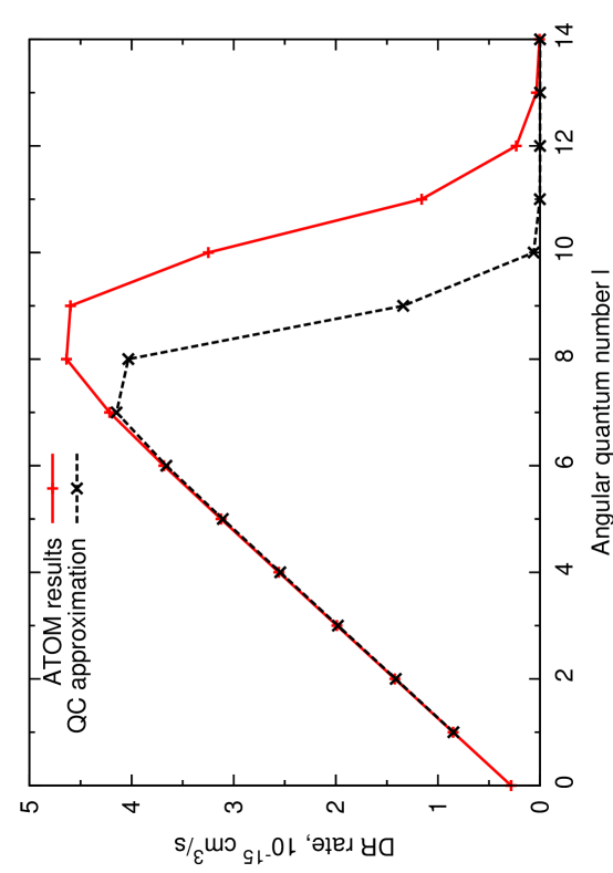
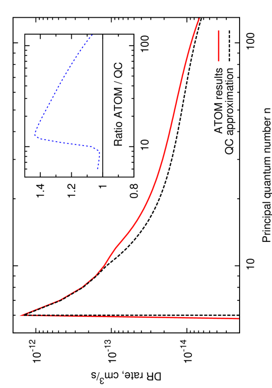
Figure 20: Comparison of $l$-resolved (upper panel) and $l$-summed (lower panel) $\@element[5+]{\mathrm{O}}$ ion dielectronic recombination rates computed by the two methods described in the text: ATOM program and quasiclassical (QC) approximation. The values are given for $T_{\rm e}=2\times 10^{4}$ K, but the curves scale identically with the temperature as long as $T_{\rm e}\ll 10^{6}$ K, when $\Delta n_{c}>0$ core excitations start playing a role. The $l$-resolved rates are given for $n=20$.

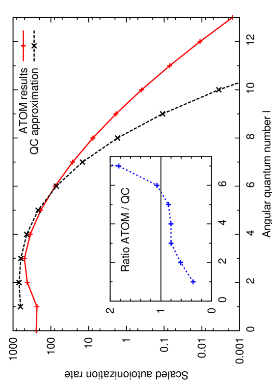
Figure 21: Comparison of scaled autoionization rates of $\@element[4+]{\mathrm{O}}$ ion in $(2p,nl)$ state autoionizing to $\@element[5+]{\mathrm{O}}$ ion in $2s$ state, $A_{\rm a}(2p,nl;2s)\times n^{3}$, $10^{13}$ s^-1, in the quasiclassical approximation and computed by the program ATOM.

Comparison of the dielectronic recombination rates with other atomic process rates is shown on Figure 22 for the case of $\@element[4+]{\mathrm{O}}$ ion with highly-excited electron on levels $n=50$ and 200. It is seen that the dielectronic recombination populates lower $l$’s, but is more efficient at high-$n$ levels. In case of sufficiently high density the dielectronic recombination to low-$l$ states is followed by rapid redistribution onto much higher $l$’s resulting in enhancement of the recombination line intensities.

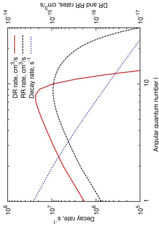
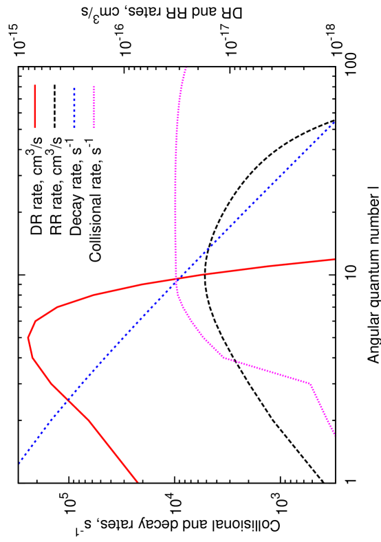
Figure 22: Elementary process rates for $\@element[5+]{\mathrm{O}}$ ion recombining to form $\@element[4+]{\mathrm{O}}$ with highly-excited electron having $n=50$ (upper panel) and $n=200$ (lower panel) at electron temperature $T_{\rm e}=2\times 10^{4}$ K. Collisional rates (total for transitions to all $l^{\prime}$) are shown for electron density $n_{\rm e}=5\times 10^{4}$ cm^-3 and are negligibly low for $n=50$ case.

B.3 Highly-excited level energies

In hydrogen atom the energies of $(nl)$ levels are independent on $l$ because of the shape of the Coulomb potential. In atoms with several electrons the changes in the potential energy curve introduce variations of the highly-excited level energies $E(nl)$ with $l$. This dependence is usually parametrized by expression

$$E(nl)={\rm Ry}\frac{z^{2}}{(n-\mu_{nl})^{2}},$$

where $\mu_{nl}$ denotes quantum defect of the level $(nl)$ and $z=Z+1$ is the ion spectroscopic symbol. The quantum defects $\mu_{nl}$ rapidly decrease with increasing $l$ and tend to constant with increasing $n$ (Seaton, 1983).

Their values are important in this study for two reasons. Firstly, level energies $E(nl)$ and $E(n^{\prime}l^{\prime})$ determine transition energies $E(nl)-E(n^{\prime}l^{\prime})$ and, therefore, spectral line wavelengths. Transitions having the same values of $n$ and $n^{\prime}$ have similar wavelengths. Small wavelength differences are in this case determined by the energy differences within $n$ and $n^{\prime}$ groups of states – by the quantum defects of the levels.

Secondly, the collisional transition rates $C_{nl,nl^{\prime}}$ are dependent on the energy level splitting $|E(nl)-E(nl^{\prime})|$, growing as this splitting decreases. Therefore the quantum defects in this case determine rates of $l$-redistribution and recombination line flux dependence on electron density in plasma.

In case of $l\leq 2$ the quantum defects for most ions are known and have been taken for our study from Ralchenko et al. (2007). In the next subsection we describe our method of computation of level energy shift from hydrogenic values $E_{\rm H}(nl)={\rm Ry}\,z^{2}/n^{2}$ for $l>2$ that can be expressed via quantum defects as

$$\Delta E(nl)\equiv E(nl)-E_{\rm H}(nl)\approx 2{\rm Ry}\frac{z^{2}}{n^{3}}\mu_{l},$$

where we have assumed that $\mu_{nl}=\mu_{l}$, i.e. that the quantum defect does not depend on $n$ and that it is small: $\mu_{l}\ll 1$.

The latter assumption is valid in our case of $l\gg 1$, when the $(nl)$ states are “non-penetrating”, i.e., those in which highly-excited electron wave function significantly differs from zero only outside the atomic core region. This property also allows to use hydrogenic expressions for description of such highly-excited states.

B.4 Computation of the level shifts for high-$l$ states

Following the approach of Watson et al. (1980) and Dickinson (1981), we account for the non-penetrating $(nl)$ state level shifts arising due to two effects: core polarizability and electrostatic quadrupole interaction with the core.

The energy shift induced by the core polarizability is proportional to the highly-excited electron radial integral $\left\langle r_{nl}^{-4}\right\rangle$ and, expressing it with hydrogenic formula, equals (Seaton, 1983)

$$\Delta E_{\rm p}(nl)=\frac{\alpha_{\rm c}}{a_{0}^{3}}\frac{z^{4}}{n^{3}}\frac{2(3-l(l+1)/n^{2})}{l(l+1)(2l-1)(2l+1)(2l+3)}{\rm Ry}.$$ (8)

Here $a_{0}$ is the Bohr radius and $\alpha_{\rm c}$ is the core polarizability, taken for relevant ions from the handbook of Fraga et al. (1976) and review by Lundeen (2005) and given for reference in Table 5.

Table 5: Atomic parameters used for computations of the line substructure.

Ion	$\left\langle r_{\rm c}^{2}\right\rangle$	$\alpha_{\rm c}$	Ion	$\left\langle r_{\rm c}^{2}\right\rangle$	$\alpha_{\rm c}$	Ion	$\left\langle r_{\rm c}^{2}\right\rangle$	$\alpha_{\rm c}$
O ii	1.20	1.35	Si ii	4.33	11.7	S ii	3.72	7.36
O iii	0.97	0.94	Si iii	3.79	7.42	S iii	3.22	4.79
O iv	0.99	0.74	Si iv		0.20	S iv	2.44	3.24
O v	0.89	0.27				S v	2.24	1.28
O v		0.007				S vi		0.07

Note. Values are given in atomic units ($a_{0}^{2}$ for $\left\langle r_{\rm c}^{2}\right\rangle$ and $a_{0}^{3}$ for $\alpha_{\rm c}$). Column “ion” contains the ion spectroscopic symbol.

The electrostatic quadrupole interaction is absent for core states having total electronic angular momentum $J_{\rm c}<1$ or total orbital momentum $L_{\rm c}<1$. If $J_{\rm c}\geq 1$, the highly-excited electron interacts with it, splitting the $(nl)$ level into $2J_{\rm c}+1$ components numbered by the quantum number $K$, where $\@vec{K}=\@vec{J}_{\rm c}+\@vec{l}$. Normally, if the $K$-splitting is present, it is larger than the level shift due to core polarizability (Lundeen, 2005).

The quadrupole shift in this case is given by the expression (Chang, 1984):

$$\begin{array}[]{l}\Delta E_{\rm q}(nl,K)=(-1)^{l+L_{\rm c}+S_{\rm c}+K}(2J_{\rm c}+1)\,{\left\{\begin{array}[]{ccc}J_{\rm c}&J_{\rm c}&2\\ L_{\rm c}&L_{\rm c}&S_{\rm c}\end{array}\right\}}\times\\ \quad\times\,{\left\{\begin{array}[]{ccc}J_{\rm c}&J_{\rm c}&2\\ l&l&K\end{array}\right\}}\;(l||C^{(2)}||l)\;(L_{\rm c}||C^{(2)}||L_{\rm c})\;\left\langle r_{\rm c}^{2}\right\rangle\;\left\langle r_{nl}^{-3}\right\rangle 2{\rm Ry},\end{array}$$ (9)

where $S_{\rm c}$ is the total core spin momentum, $\left\{:\;:\;:\right\}$ denote a $6j$-symbol, $\left\langle r_{\rm c}^{2}\right\rangle$ and $\left\langle r_{nl}^{-3}\right\rangle$ are radial integrals in atomic units for core and highly-excited electron, respectively, and $(l||C^{(2)}||l)$’s are reduced matrix elements, given explicitly, e.g., by Sobelman (1979):

$$(l||C^{(2)}||l)=-\sqrt{\frac{l(l+1)(2l+1)}{(2l+3)(2l-1)}}.$$

The highly-excited electron radial integral can be determined using hydrogenic expression from, e.g., Bethe & Salpeter (1957). Core radial integrals $\left\langle r_{\rm c}^{2}\right\rangle$ were computed for all relevant ions using radial wave functions produced by the Flexible Atomic Code (FAC, Gu (2003)). Where literature data for the $\left\langle r_{\rm c}^{2}\right\rangle$ were available (Sen, 1979), the differences between them and the FAC values did not exceed about 10-15%. The used values of the $\left\langle r_{\rm c}^{2}\right\rangle$ are given in Table 5.

Expression (9) may be approximated in case of P core states ($L_{\rm c}=1$) and $l\gg 1$ by

$$\Delta E_{\rm q,\,max}(nl) \approx 0.2\,\left\langle r_{\rm c}^{2}\right\rangle\,\left\langle r_{nl}^{-3}\right\rangle{\rm Ry}$$ (10)

$$= {}0.2\frac{z^{3}\left\langle r_{\rm c}^{2}\right\rangle}{n^{3}l(l+1)(l+1/2)}{\rm Ry},$$

where in this case $\Delta E_{\rm q,\,max}(nl)$ gives maximum shift of all the $K$-components. Components with both $\Delta E_{\rm q,\,max}(nl)$ and $-\Delta E_{\rm q,\,max}(nl)$ shifts are sometimes present.

Taking into account these effects, the total $(nl)$ state shift for estimate of the collisional $l$-redistribution rates was taken to be maximum possible, i.e.,

$$\Delta E(nl)=\Delta E_{\rm q,\,max}(nl)+\left|\Delta E_{\rm p}(nl)\right|.$$

As larger shifts correspond to smaller collisional cross sections, our approach may somewhat underestimate the $l$-redistribution rates.

We estimate that the resulting uncertainties of level splittings, in case of the $K$-splitting present, correspond to the uncertainties in the electron density determination from the line ratios (see Section 5.2) being within a factor of about two.

B.5 Computation of the line substructure

As the ions of different elements have different values of $\alpha_{\rm c}$ and $\left\langle r_{\rm c}^{2}\right\rangle$, the recombination line exact wavelengths will depend not only on the ionic charge and the principal quantum numbers of the transition, but also on the element and the quantum numbers $l$, $l^{\prime}$, $K$ and $K^{\prime}$.

From the above expressions determining energy levels shifts it is possible to calculate the positions of all line $nl\to n^{\prime}l^{\prime}$ components $nlK\to n^{\prime}l^{\prime}K^{\prime}$. Their relative fluxes are determined by the so-called line strengths $S$ according to expression (Chang, 1984)

$$S(nlK,n^{\prime}l^{\prime}K^{\prime})\propto(2K^{\prime}+1)(2K+1)\,{\left\{\begin{array}[]{ccc}K^{\prime}&K&1\\ l&l^{\prime}&J_{\rm c}\end{array}\right\}^{2}},$$ (11)

if we assume that populations of the $(nlK)$-states are proportional to their statistical weights equal to $(2K+1)$.

It was shown by Chang (1984) that $l=3$ levels in Si i are still partially penetrating the core. Therefore also in our case the Si and S line substructure is described adequately only for $l>3$. In our paper we give results also for $l=3$, but the precision of line position predictions in this case is expected to be rather limited.

In the post-shock plasma of the fast moving knots, the density is high enough to establish significant population of lowest excited fine-structure sublevels (Smeding & Pottasch, 1979) that have typical excitation energies corresponding to temperatures of several hundred Kelvin.

In some cases such excited state populations strongly change the line substructure. For example, in $\@element[3+]{\mathrm{O}}$ ion, the ground state ${}^{2}P_{1/2}$ has $J_{\rm c}=1/2$ and quadrupole interaction with it is absent. Though, the lowest excited state ${}^{2}P_{3/2}$ of this ion has $J_{\rm c}=3/2$. In case the core electron is in the excited state prior to recombination, or getting there after the DR process, the highly-excited levels will have $K$-splitting and resulting recombination lines will have much richer substructure.

In our analysis we assume populations of the $J_{\rm c}$ sublevels proportional to their statistical weights.

B.6 Line emission without recombination

We also account for the following process, mostly not resulting in a recombination, but contributing, sometimes noticeably, to the spectral line emissivities:

$$X^{Z+}(\gamma_{0})+e \rightleftarrows X^{(Z-1)+}(\gamma,nl)\to$$

$$\to X^{(Z-1)+}(\gamma,n^{\prime}l^{\prime})+{\rm photon}\to$$

$$\to X^{Z+}(\gamma_{0})+e^{\prime}+{\rm photon},$$

i.e., highly-excited electron transition instead of core transition, followed by the captured electron autoionization. This process may be quite efficient for increasing $\Delta n=1$ transition emissivities, as the radiative transition rates for captured electron may be significantly higher than that of the core electron, if the core transition rate is low.

This is exactly the case for $\Delta n_{\rm c}=0$ transitions, mostly contributing to the DR at relatively low temperatures. Rate of the described process (“dielectronic capture with line emission”, DCL) forming a line from transition $(nl)\to(n^{\prime}l^{\prime})$ may be easily expressed via the rate of the dielectronic recombination as

$$q_{\rm DCL}(\gamma,nl,n^{\prime}l^{\prime};T_{\rm e})=q_{\rm DR}(\gamma,nl;T_{\rm e})\;\frac{A_{nl,n^{\prime}l^{\prime}}}{A_{\rm c}}.$$ (13)

As the autoionization rates are much higher than the radiative transition rates within the ion, probability of the DCL is small and after the first captured electron transition it autoionizes, if it is energetically allowed.

To produce noticeable effect, highly-excited electron transition rates should be at least comparable to the core transition rates, as DCL does not produce cascades. Therefore, only transitions between lower $n$’s contribute significantly to the additional emission in lines. In case of $\@element[5+]{\mathrm{O}}$, described process increases the DR contribution to the recombination line emissivity by roughly 5% for the $8\alpha$ and $7\alpha$ lines. From Eq. (13) it is clear that this fraction does not depend on temperature.

B.7 Estimates of the resulting uncertainties

Given the amount of approximations made to achieve the final results – the metal recombination line emissivities and wavelengths – it might be useful to state explicitly resulting uncertainties of these quantities.

The least reliable components for calculation of the recombination line emissivities are dielectronic recombination rates and upper cutoff position.

For the ions where the ATOM results are available, the low-density emissivity and flux uncertainties are expected to be about 10%. For the ions where the calculations are made using the quasiclassical expressions, the precision is lower and may constitute up to 50%.

The choice of the upper cutoff $n_{\rm max}$ position results in additional emissivity uncertainty of less than 10% for the DR-dominated recombinations and emissivity underestimate of less than 20% for the RR-dominated case.

The density dependences of the line emissivities are not strong and should be quite reliably modeled with additional uncertainties being below 5–10%.

It should be reiterated that the absolute oxygen line fluxes are much less confidently predicted, as their values are based on the theoretical FMK model that shows differences when compared to the observed optical-to-infrared collisional line ratios up to a factor of several (Docenko & Sunyaev, to be submitted).

The line fine structure uncertainties are coming from the input atomic data (polarizabilities and radial integrals) limited precision. It is estimated to be not larger than 10–20%, thus the line fine structure should be quite reliable.

The recombination line fine structure component relative intensities are the least reliably predicted as they depend on the recombining ion ground state populations. The results given above assume equilibrium populations; this may not be true at low densities or temperatures. Therefore the observed line structure may be significantly different from one expected. From another side, observed line structure will allow to put additional constraints on the electron density and temperature from the fine structure component intensities.

References

- Baade & Minkowski (1954) Baade, W. & Minkowski, R. 1954, Astrophys. J., 119, 206
- Beigman et al. (1981) Beigman, I. L., Vainshtein, L. A., & Chichkov, B. N. 1981, Soviet Physics JETP, 3, 490
- Beigman et al. (1968) Beigman, I. L., Vainshtein, L. A., & Sunyaev, R. A. 1968, Soviet Physics Uspekhi, 11, 411
- Bethe & Salpeter (1957) Bethe, H. A. & Salpeter, E. E. 1957, Quantum Mechanics of One- and Two-Electron Atoms (New York: Academic Press)
- Blum & Pradhan (1992) Blum, R. D. & Pradhan, A. K. 1992, Astrophys. J. Suppl. Ser., 80, 425
- Borkowski & Shull (1990) Borkowski, K. J. & Shull, J. M. 1990, Astrophys. J., 348, 169
- Brault & Noyes (1983) Brault, J. & Noyes, R. 1983, Astrophys. J., 269, L61
- Bureyeva & Lisitsa (2000) Bureyeva, L. A. & Lisitsa, V. S. 2000, Astrophysics and Space Physics Reviews, 11, 1
- Chang (1984) Chang, E. S. 1984, Journal of Physics B: Atomic and Molecular Physics, 17, L11
- Chang & Noyes (1983) Chang, E. S. & Noyes, R. W. 1983, Astrophys. J., 275, L11
- Chevalier & Kirshner (1978) Chevalier, R. A. & Kirshner, R. P. 1978, Astrophys. J., 219, 931
- Chevalier & Kirshner (1979) Chevalier, R. A. & Kirshner, R. P. 1979, Astrophys. J., 233, 154
- Dere et al. (1997) Dere, K. P., Landi, E., Mason, H. E., Monsignori Fossi, B. C., & Young, P. R. 1997, Astron. Astrophys. Suppl. Ser., 125, 149
- Dickinson (1981) Dickinson, A. S. 1981, Astron. Astrophys., 100, 302
- Dopita et al. (1984) Dopita, M. A., Binette, L., & Tuohy, I. R. 1984, Astrophys. J., 282, 142
- Fraga et al. (1976) Fraga, S., Karkowski, J., & Saxena, K. M. S. 1976, Handbook of Atomic Data (Elsevier, Amsterdam)
- Gerardy & Fesen (2001) Gerardy, C. L. & Fesen, R. A. 2001, Astron. J., 121, 2781
- Gordon (1929) Gordon, W. 1929, Annalen der Physik, 394, 1031
- Gu (2003) Gu, M. F. 2003, Astrophys. J., 582, 1241
- Heng & McCray (2007) Heng, K. & McCray, R. 2007, Astrophys. J., 654, 923
- Hughes et al. (2000) Hughes, J. P., Rakowski, C. E., Burrows, D. N., & Slane, P. O. 2000, Astrophys. J., 528, L109
- Hurford & Fesen (1996) Hurford, A. P. & Fesen, R. A. 1996, Astrophys. J., 469, 246
- Hwang et al. (2004) Hwang, U., Laming, J. M., Badenes, C., et al. 2004, Astrophys. J., 615, L117
- Inogamov & Sunyaev (2003) Inogamov, N. A. & Sunyaev, R. A. 2003, Astronomy Letters, 29, 791
- Itoh (1981a) Itoh, H. 1981a, Publ. Astron. Soc. Japan, 33, 1
- Itoh (1981b) Itoh, H. 1981b, Publ. Astron. Soc. Japan, 33, 521
- Itoh (1986) Itoh, H. 1986, Publ. Astron. Soc. Japan, 38, 717
- Klein et al. (2003) Klein, R. I., Budil, K. S., Perry, T. S., & Bach, D. R. 2003, Astrophys. J., 583, 245
- Landi et al. (2006) Landi, E., Del Zanna, G., Young, P. R., et al. 2006, Astrophys. J. Suppl. Ser., 162, 261
- Lennon & Burke (1994) Lennon, D. J. & Burke, V. M. 1994, Astron. Astrophys. Suppl. Ser., 103, 273
- Lundeen (2005) Lundeen, S. R. 2005, Advances in Atomic, Molecular, and Optical Physics, Vol. 52, Fine Structure in High- Rydberg states: A Path to Properties of Positive Ions (Academic Press, edited by Chun C. Lin and Paul Berman), 161–208
- Malik et al. (1991) Malik, G. P., Malik, U., & Varma, V. S. 1991, Astrophys. J., 371, 418
- Mazzotta et al. (1998) Mazzotta, P., Mazzitelli, G., Colafrancesco, S., & Vittorio, N. 1998, Astron. Astrophys. Suppl. Ser., 133, 403
- McKee & Cowie (1975) McKee, C. F. & Cowie, L. L. 1975, Astrophys. J., 195, 715
- Minkowski (1957) Minkowski, R. 1957, in IAU Symposium, Vol. 4, Radio astronomy, ed. H. C. van de Hulst, 107
- Minkowski & Aller (1954) Minkowski, R. & Aller, L. H. 1954, Astrophys. J., 119, 232
- Peimbert & van den Bergh (1971) Peimbert, M. & van den Bergh, S. 1971, Astrophys. J., 167, 223
- Pengelly & Seaton (1964) Pengelly, R. M. & Seaton, M. J. 1964, MNRAS, 127, 165
- Pequignot et al. (1991) Pequignot, D., Petitjean, P., & Boisson, C. 1991, Astron. Astrophys., 251, 680
- Ralchenko et al. (2007) Ralchenko, Y., Jou, F.-C., Kelleher, D., et al. 2007, National Institute of Standards and Technology, Gaithersburg, MD
- Schild (1977) Schild, R. E. 1977, Astron. J., 82, 337
- Seaton (1983) Seaton, M. J. 1983, Reports of Progress in Physics, 46, 167
- Seaton & Storey (1976) Seaton, M. J. & Storey, P. J. 1976, in Atomic processes and applications. P. G. Burke (ed.), North-Holland Publ. Co., Amsterdam, Netherlands, 133–197
- Sen (1979) Sen, K. D. 1979, Phys. Rev. A, 20, 2276
- Shevelko & Vainshtein (1993) Shevelko, V. P. & Vainshtein, L. A. 1993, Atomic physics for hot plasmas (Bristol: IOP Publishing)
- Shklovskii (1968) Shklovskii, I. S. 1968, Supernovae (London, New York, etc.: Wiley)
- Shore (1969) Shore, B. W. 1969, Astrophys. J., 158, 1205
- Smeding & Pottasch (1979) Smeding, A. G. & Pottasch, S. R. 1979, Astron. Astrophys. Suppl. Ser., 35, 257
- Sobelman (1979) Sobelman, I. I. 1979, Atomic spectra and radiative transitions (Springer Series in Chemical Physics, Berlin: Springer)
- Sobelman et al. (1981) Sobelman, I. I., Vainshtein, L. A., & Yukov, E. A. 1981, Excitation of atoms and broadening of spectral lines (Springer Series in Chemical Physics 7, Berlin: Springer)
- Spitzer (1956) Spitzer, L. 1956, Physics of Fully Ionized Gases (New York: Interscience Publishers)
- Storey & Hummer (1991) Storey, P. J. & Hummer, D. G. 1991, Computer Physics Communications, 66, 129
- Summers (1977) Summers, H. P. 1977, MNRAS, 178, 101
- Sutherland & Dopita (1995a) Sutherland, R. S. & Dopita, M. A. 1995a, Astrophys. J., 439, 365
- Sutherland & Dopita (1995b) Sutherland, R. S. & Dopita, M. A. 1995b, Astrophys. J., 439, 381
- Tayal (2000) Tayal, S. S. 2000, Astrophys. J., 530, 1091
- Tayal (2006) Tayal, S. S. 2006, Astrophys. J. Suppl. Ser., 166, 634
- Tayal & Gupta (1999) Tayal, S. S. & Gupta, G. P. 1999, Astrophys. J., 526, 544
- van den Bergh (1971) van den Bergh, S. 1971, Astrophys. J., 165, 457
- Vrinceanu & Flannery (2001) Vrinceanu, D. & Flannery, M. R. 2001, Phys. Rev. A, 63, 032701
- Watson et al. (1980) Watson, W. D., Western, L. R., & Christensen, R. B. 1980, Astrophys. J., 240, 956
- Zel’dovich & Raizer (1967) Zel’dovich, Y. B. & Raizer, Y. P. 1967, Physics of shock waves and high-temperature hydrodynamic phenomena (New York: Academic Press, edited by Hayes, W.D.; Probstein, Ronald F.)