Enhanced Geometry Fluctuations in Minkowski and Black Hole Spacetimes

Abstract

We will discuss selected physical effects of spacetime geometry fluctuations, especially the operational signatures of geometry fluctuations and their effects on black hole horizons. The operational signatures which we discuss involve the effects of the fluctuations on images, and include luminosity variations, spectral line broadening and angular blurring. Our main interest will be in black hole horizon fluctuations, especially horizon fluctuations which have been enhanced above the vacuum level by gravitons or matter in squeezed states. We investigate whether these fluctuations can alter the thermal character of a black hole. We find that this thermal character is remarkably robust, and that Hawking’s original derivation using transplanckian modes does not seem to be sensitive even to enhanced horizon fluctuations.

1 Introduction

In this paper, we will discuss selected aspects of the effects of quantum spacetime geometry fluctuations, using the Riemann tensor correlation function as our basic tool. It is first useful to make a distinction between active fluctuations, which arise from the dynamical degrees of freedom of gravity itself, and passive fluctuations, which are driven by quantum stress tensor fluctuations of matter fields. In general, both types of fluctuations are present. We will be concerned with the case where the fluctuations around a classical background spacetime are small, so we can consider each type separately and add their effects. Of course, a full treatment of active fluctuations would require a more complete theory of quantum gravity than currently exists, but we restrict our attention to quantized linear perturbations of the background spacetime.

Various aspects of spacetime geometry fluctuations have been discussed by several authors in recent years, for example  [1, 2, 3, 4, 5, 6, 7, 8, 9, 10, 11, 12]. In particular, stochastic gravity [13] has been studied as a systematic approach to go beyond the semiclassical theory. In the present paper, we will concentrate on two issues. The first is some phenomenological effects of geometry fluctuations in a nearly flat background, which will be discussed in Section 2. Here we will be summarising work that was previously published [14, 15]. The second issue will be the possibility of enhancing horizon fluctuations by use of squeezed states, discussed in Section 5. Here we will be summarising work that will developed in more detail in a forthcoming paper [16].

2 Phenomenology of Riemann Tensor Fluctuations

In this section, we will briefly review some of the operational signatures of spacetime geometry fluctuations, and describe how these may be given a geometrical description in terms of the Riemann tensor correlation function. Here we direct our attention to the case of a nearly flat background, but the same techniques can be used in more general spacetimes.

2.1 Luminosity Fluctuations

The image of a source viewed through a fluctuating medium can undergo variations in apparent brightness. This effect is known to astronomers as scintillation, and to the general public as “twinkling”. The most familiar example arises when stars are viewed through the earth’s atmosphere, which is undergoing density fluctuations. In the case of fluctuations of the spacetime geometry, this effect may be studied using the Raychaudhuri equation as a Langevin equation [14, 17]. One calculates fluctuations of the expansion $\theta$. In the case that the shear, vorticity, and squared expansion can be neglected, this equation becomes

$$\frac{d\theta}{d\lambda}=-R_{\mu\nu}k^{\mu}k^{\nu}\,,$$ (1)

where $\lambda$ is an affine parameter, $k^{\mu}$ is the tangent to the geodesic congruence, and $R_{\mu\nu}$ is the Ricci tensor. If the expansion vanishes at $\lambda_{0}$, then the variance of the expansion becomes

$$\langle\theta^{2}\rangle-\langle\theta\rangle^{2} = \langle(\Delta\theta)^{2}\rangle=\int_{0}^{\lambda_{0}}d\lambda\int_{0}^{\lambda_{0}}d\lambda^{\prime}$$ (2)

$$\times C_{\mu\nu\alpha\beta}(\lambda,\lambda^{\prime})\,k^{\mu}(\lambda)k^{\nu}(\lambda)\,k^{\alpha}(\lambda^{\prime})k^{\beta}(\lambda^{\prime})\,,$$

where

$$C_{\mu\nu\alpha\beta}(x,x^{\prime})=\langle R_{\mu\nu}(x)R_{\alpha\beta}(x^{\prime})\rangle-\langle R_{\mu\nu}(x)\rangle\langle R_{\alpha\beta}(x^{\prime})\rangle$$ (3)

is the Ricci tensor correlation function. It is obtained by appropriate contractions of the Riemann tensor correlation function and is determined by the stress tensor correlation function. Thus we see that luminosity fluctuations, in lowest order, are signatures of passive fluctuations. The results of several explicit models are given in [14].

2.2 Line Broadening and Angular Blurring

Two other effects which can arise when a source is viewed through a fluctuating spacetime geometry are broadening of spectral lines and blurring of images. Both of these effects may be given a unified geometric treatment, which we summarise here. Consider a source which is sending successive pulses to a detector as illustrated in Figure 1.

Figure 1: A source moves along a worldline with tangent $t^{\mu}$ while a detector a proper distance $s$ away moves along a worldline with tangent $v^{\mu}$. The source emits a ray which has tangent $k^{\mu}(\lambda=0)$ at point D and tangent $k^{\mu}(\lambda_{0})$ at A. Parallel propagation of $k^{\mu}$ around ABCD results in a slightly rotated vector $k^{\mu}+\Delta k^{\mu}$. The closed path ABCD encloses the spacetime region of interest.

The effect of the spacetime geometry is to cause a shift $\Delta k^{\mu}$ between successive pulses. This shift can be expressed as an integral of the Riemann tensor over the region illustrated:

$$\Delta k^{\mu}=-\int_{\tau_{1}}^{\tau_{2}}d\tau\int_{0}^{\lambda_{0}}d\lambda\,R^{\mu}_{\phantom{\mu}\alpha\nu\beta}k^{\alpha}t^{\nu}k^{\beta}\,.$$ (4)

A shift in the time component is observed as a frequency shift, whereas as shift in a spatial component produces a shift in position of the image. Fluctuations of the geometry lead to variations in each of these quantities. Denote the fractional line broadening by $\Delta\xi=\Delta\omega/\omega$. Its variance can be expressed as

$$\delta\xi^{2}=\langle(\Delta\xi)^{2}\rangle-\langle\Delta\xi\rangle^{2}=\int da\int da^{\prime}\,C_{\alpha\beta\mu\nu\,\gamma\delta\rho\sigma}(x,x^{\prime})t^{\alpha}k^{\beta}t^{\mu}k^{\nu}t^{\gamma}k^{\delta}t^{\rho}k^{\sigma}.$$ (5)

Here

$$C_{\alpha\beta\mu\nu\,\gamma\delta\rho\sigma}(x,x^{\prime})=\langle R_{\alpha\beta\mu\nu}(x)R_{\gamma\delta\rho\sigma}(x^{\prime})\rangle-\langle R_{\alpha\beta\mu\nu}(x)\rangle\langle R_{\gamma\delta\rho\sigma}(x^{\prime})\rangle$$ (6)

is the Riemann tensor correlation function. Similarly the fluctuations of an image’s angular position in a direction defined by the spacelike vector $s^{\mu}$ are given by.

$$\delta\Theta^{2} = \langle(\Delta\Theta)^{2}\rangle-\langle\Delta\Theta\rangle^{2}=\int da\int da^{\prime}$$ (7)

$$\times C_{\alpha\beta\mu\nu\,\gamma\delta\rho\sigma}(x,x^{\prime})s^{\alpha}k^{\beta}t^{\mu}k^{\nu}s^{\gamma}k^{\delta}t^{\rho}k^{\sigma}.$$

Several explicit examples of these effects, including enhanced fluctuations due to gravitons in squeezed states, are discussed in [15] .

3 Black Hole Evaporation

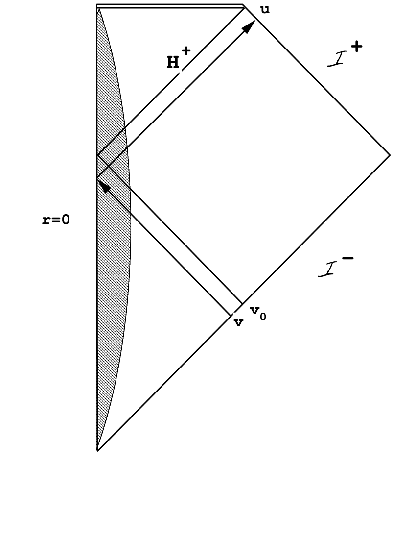
Figure 2: The spacetime of a black hole formed by gravitational collapse is illustrated. The shaded region is the interior of the collapsing body, the $r=0$ line on the left is the worldline of the center of this body, the $r=0$ line at the top of the diagram is the curvature singularity, and $H^{+}$ is the future event horizon. An ingoing light ray with $v<v_{0}$ from ${\cal I^{-}}$ passes through the body and escapes to ${\cal I^{+}}$ as a $u=constant$ light ray. Ingoing rays with $v>v_{0}$ do not escape and eventually reach the singularity.

In this section, we will briefly review Hawking’s derivation [18] of black hole evaporation. The basic idea is to consider the spacetime of a black hole formed by gravitational collapse, as illustrated in Figure 2. A quantum field propagating in this spacetime is assumed to be in the in-vacuum state, that is, containing no particles before the collapse. In the case of a massless field, a purely positive frequency mode proportional to ${\rm e}^{-i\omega v}$ leaves $\cal{I}^{-}$, propagates through the collapsing body, and reaches $\cal{I}^{+}$ after undergoing a large redshift in the region outside of the collapsing matter. At $\cal{I}^{+}$, the mode is now a mixture of positive and negative frequency parts, signalling quantum particle creation. Of special interest are the modes which leave $\cal{I}^{-}$ just before the formation of the horizon, which is the $v=v_{0}$ ray. These modes give the dominant contribution to the outgoing flux at times long after the black hole has formed. After passing through the collapsing body, they are $u$= constant rays, where

$$u=-4M\,\ln\biggl{(}{{v_{0}-v}\over C}\biggr{)}\,,$$ (8)

where $M$ is the black hole’s mass, and $C$ is a constant. The logarithmic dependence leads to a Planckian spectrum of created particles. It also leads to what some authors call the “transplanckian problem”. We prefer to refer it as the “transplanckian issue”, as in our view there may not be any problem. In any case, this is the enormous frequency which the dominant modes must have when they leave $\cal{I}^{-}$. The typical frequency of the radiated particles reaching $\cal{I}^{+}$ midway through the evaporation process is of order $1/M$, but the typical frequency of these modes at $\cal{I}^{-}$ is of order

$$\omega\approx M^{-1}{\rm e}^{(M/M_{Pl})^{2}}\,,$$ (9)

where $M_{Pl}$ is the Planck mass. Another way to state this is to note that the characteristic value of $u$ for these modes is of order

$$u_{c}\approx M\biggl{(}\frac{M}{m_{p}}\biggr{)}^{2}\,.$$ (10)

A geodesic observer who falls from rest at large distance from the black hole will pass from $u=u_{c}$ to the horizon at $u=\infty$ in a proper time of

$$\delta\tau\approx M\,e^{-{u_{c}}/{4M}}\approx M\,e^{-{M^{2}}/{m_{p}^{2}}}\,.$$ (11)

which is far smaller than the Planck time. In this sense, the outgoing modes are much less than a Planck length outside the horizon.

Several authors, especially Unruh [19, 20] and Jacobson [21, 22] have noted that it is possible to avoid the use of transplanckian modes provided that the dispersion relation for the quantum field is suitably modified. This can lead to the phenomenon of “mode regeneration”, whereby the modes which become occupied by the thermal radiation do not arise by red-shifting of transplanckian modes, but rather are generated by nonlinear effects just before they are due to be occupied. This possibility has the benefit of avoiding transplankian frequencies, but the drawback that it requires violation of local Lorentz invariance, and hence would depend upon as yet undiscovered physics.

For the case of a bosonic field, spontaneous emission implies the possibility of stimulated emission. However, in the picture described by the original Hawking derivation, stimulated emission into modes with wavelengths of order $1/M$ require one to start with an initial state which is populated by particles with transplanckian frequencies. The possibility of stimulated emission in the case of the Hawking effect was first discussed by Wald [23].

4 Horizon Fluctuations

We now turn to the central issue of this paper, that of black hole horizon fluctuations. In classical general relativity, the event horizon is the history of the light ray which is marginally trapped by the black hole. It gives a sharp boundary between events which are visible to the outside, and those which are not. However, in quantum physics, one does not expect such sharp boundaries, but rather a smeared horizon due to quantum fluctuation effects. Several authors have discussed this possibility from different viewpoints  [24, 25, 26, 27, 28, 29, 30, 31]. One approach is to calculate fluctuations in the horizon area [24, 25, 26]. Another [29] is to study the variation in the times at which rays just outside the classical horizon arrive at a distant observer. It is the latter approach which will adopted in the present paper.

A crucial question is whether quantum horizon fluctuations will significantly alter the Hawking derivation outlined above. Given that the outgoing modes which eventually become populated with the thermal radiation spend part of their history less than a Planck length outside the mean horizon, it would seem at first that horizon fluctuations could drastically change the result. Fluctuations on the Planck scale would seem to cause a significant fraction of the outgoing modes either to fall into the black hole and never reach $\cal{I}^{+}$, or else to be ejected prematurely. In either case, the thermal character of the Hawking radiation would seem to be greatly changed. This would upset the elegant connection between black hole physics, thermodynamics, and quantum theory. In fact, the situation is not so dire as it first seems. Ford and Svaiter [29] gave an estimate of the effects of the active fluctuations when the graviton field is in its vacuum state. They found that the effects are quite small for black holes whose mass is above the Planck scale. Specifically, they calculated variations in the time $\delta\tau$ given in (11) due to the quantum metric fluctuations and found that these fractional variations are small so long as $M\gg m_{Pl}$.

5 Enhanced Horizon Fluctuations

Squeezed states are capable of enhancing quantum fluctuations beyond the vacuum level. This raises the possibility of increasing the horizon fluctuations of a black hole by sending in quantum fields in a squeezed vacuum state. In the remainder of this paper, we will discuss three models for the source of the fluctuations. However, first we outline a geometric approach to study the effects of geometry fluctuations on the horizon. The basic idea is to study the geodesic deviation of the outgoing null geodesics just outside the mean horizon.

Figure 3: Schwarzschild black hole space-time formed via gravitational collapse. The separation vector characterizing geodesic deviation of the horizon, $\cal{H}^{+}$, and a nearby outgoing null geodesic, $\gamma$, is initially $n^{\nu}=n^{\nu}_{0}$ but then evolves as $n^{\nu}=n^{\nu}_{0}+\delta_{s}n^{\mu}$. The vector $\ell^{\mu}$ is tangent to the horizon.

This is illustrated in Figure 3. Here $n^{\mu}$ is the separation vector which describes the peeling of the outgoing geodesics from the horizon (which is hidden in a conformal spacetime diagram). This vector satisfies the geodesic deviation equation,

$$\frac{D^{2}n^{\alpha}}{dV^{2}}=R^{\alpha}_{\phantom{\alpha}\beta\mu\nu}\ell^{\beta}\ell^{\mu}n^{\nu}\,,$$ (12)

where $\ell^{\mu}$ is the tangent to the horizon.

We first consider the solution of this equation in the classical Schwarzschild spacetime. This is conveniently done in null Kruskal coordinates, in which the Schwarzschild metric is

$$ds^{2}=\frac{-32M^{3}}{r}e^{-r/2M}dUdV+r^{2}d\Omega^{2}\,.$$ (13)

The advantage of these coordinates is that $V$, which is constant on ingoing null rays, is an affine parameter for the horizon. Let $V=V_{0}$ be an initial point at which $n^{\mu}=n_{0}\,\delta^{\mu}_{U}$, where $n_{0}$ is a constant. Then the solution of (12) to lowest non-trivial order in $V-V_{0}$, when $r-2M\ll M$, is

$$n^{\alpha}=n_{0}^{\alpha}+\delta_{s}n^{\alpha}=n_{0}\left(1,-e^{-1}(V-V_{0})^{2}\right)\,.$$ (14)

That is, the vector $n^{\mu}$ which initially has only a $U$-component, develops a $V$-component with no change in the $U$-component to this order. The vector is null at the starting point, but afterwards is spacelike with squared norm

$$\left(n^{\mu}n_{\mu}\right)^{2}=4\left(g_{UV}\,n_{0}^{2}e^{-1}\right)^{2}\left(V-V_{0}\right)^{4}\,.$$ (15)

The growth of $n^{V}$ describes the peeling of the outgoing geodesic from the horizon.

We now wish to consider the effects of quantum geometry fluctuations. This may be done by treating (12) as a Langevin equation with a fluctuating part of the Riemann tensor, $\delta R^{\alpha}_{\phantom{\alpha}\mu\beta\nu}$. The separation vector now becomes a fluctuating vector written as

$$\bar{n}^{\alpha}=n_{0}^{\alpha}+\delta_{s}n^{\alpha}+\delta_{p}\hat{n}^{\alpha}\,,$$ (16)

where the contribution from the fluctuations, to lowest order in $V-V_{0}$, is

$$\delta_{p}\hat{n}^{\alpha}=\int_{V_{0}}^{V}dW\int_{V_{0}}^{W}dV\,\delta R^{\alpha}_{\phantom{\alpha}\mu\beta\nu}\ell^{\mu}\ell^{\beta}n_{0}^{\nu}.$$ (17)

Our measure of the effects of the quantum fluctuations will be the variance of $(\bar{n}^{\mu}\bar{n}_{\mu})^{2}$. To lowest order in $V-V_{0}$, this variance may be expressed as

$$\Delta(\bar{n}^{\mu}\bar{n}_{\mu})^{2} = 4\left[\langle\left(n^{\mu}_{0}(x)\delta_{p}\hat{n}_{\mu}(x)\right)\left(n^{\nu}_{0}(x^{\prime})\delta_{p}\hat{n}_{\nu}(x^{\prime})\right)\rangle\right.$$ (18)

$$- \left.\langle n^{\mu}_{0}(x)\delta_{p}\hat{n}_{\mu}(x)\rangle\langle n^{\nu}_{0}(x^{\prime})\delta_{p}\hat{n}_{\nu}(x^{\prime})\rangle\right].$$

Here we have used the facts that $\delta_{s}n_{\nu}(x)\propto(V-V_{0})^{2}$, and that each $\delta_{p}\hat{n}_{\nu}(x)\propto(V-V_{0})^{2}$, as will be demonstrated in each of the explicit models of fluctuations to be considered below. Note that (18) involves a double integral of the Riemann tensor correlation function, as each factor of $\delta_{p}\hat{n}_{\nu}$ is an integral over the fluctuating Riemann tensor, (17).

5.1 Scalar Graviton Model

First we discuss a simplified model which captures the essential physics of active fluctuations without the complications entailed in treating tensor perturbations in a black hole spacetime. Here the perturbed metric is taken to have the form

$$\bar{g}_{\mu\nu}=\left(1+\Phi\right)g_{\mu\nu}\,,$$ (19)

where $g_{\mu\nu}$ is the unperturbed Schwarzschild background metric and $\Phi$ is a free quantum scalar field, which we take to satisfy the minimally coupled wave equation

$$\nabla^{\mu}\nabla_{\mu}\,\Phi=0$$ (20)

in the Schwarzschild spacetime. This is sometimes called a dilaton field, but for our purposes it models the effects of gravitons. We can expand the operator $\Phi$ in terms of a complete set of positive norm wave packets solutions $\{\psi_{jn}\}$ as

$$\Phi=\sum_{jn}(\psi_{jn}\hat{a}_{jn}+\psi_{jn}^{*}\hat{a}_{jn}^{\dagger})\,,$$ (21)

where the $\hat{a}_{jn}$ are annihilation operators.

Following Hawking [18], we define the ingoing wave packets by

$$\psi_{jn}=\varepsilon_{j}^{-\frac{1}{2}}\int_{j\varepsilon_{j}}^{(j+1)\varepsilon_{j}}e^{-2\pi in\omega/\varepsilon_{j}}\psi_{\omega\ell m}\,d\omega\,,$$ (22)

where

$$\psi_{\omega\ell m}=\frac{Y_{\ell m}(\theta,\varphi)}{r\sqrt{2\pi\omega}}F_{\omega}(r)e^{-i\omega v}\,.$$ (23)

Here $v=t+r^{*}$ is the usual advanced time coordinate. The function $F(r)$ approaches unity for $r\gg M$ and approaches a constant of magnitude less than unity, the transmission coefficient, near the horizon. The integer $j$ controls where in frequency space the wave packet is peaked, while $\varepsilon_{j}$ controls the width of the wave packet and has units of frequency. The integer $n$ describes which wave packet is under consideration. This construction allows for wave packets to be sent in at regular intervals of ${2\pi}/{\varepsilon_{j}}$ with various frequencies. Thus $\psi_{jn}$ is the $n^{th}$ wave packet sent in with component frequencies ranging from $j\varepsilon_{j}$ to $(j+1)\varepsilon_{j}$. A corresponding set of outgoing packets can be defined by substitution of $u$ for $v$ in (23).

We now wish to take the quantum state of the scalar field to be a multi-mode squeezed vacuum state for some finite set of wave packet modes, which are sent into the black hole well after the collapse. Let the squeeze parameter of a given mode be $\xi_{j}=\rho_{j}\,{\rm e}^{i\delta_{j}}$, where $j$ labels the various excited modes. We are interested in the effects of the excitation, so we take the difference between the given state and the vacuum state, and also assume that $\rho_{j}\gg 1$, corresponding to highly excited states. The function $F(r)$ becomes the transmission coefficient near the horizon, where we need to evaluate it. This transmission coefficient is of order unity for wavelengths shorter than the size of the black hole, $\omega\geq(2M)^{-1}$, and is approximately $C(2i\omega M)^{\ell+1}$ when $\omega\ll(2M)^{-1}$, where $|C|$ is a constant of order unity.

In the case that $\omega\approx(2M)^{-1}$, we find the fractional fluctuations to be approximately

$$\frac{\Delta(\bar{n}^{\mu}\bar{n}_{\mu})^{2}}{(n^{\mu}n_{\mu})^{2}} = \frac{Y^{2}_{\ell 0}}{16}\,|C|^{2}\,\sum_{j}\frac{e^{2\rho_{j}}\ell^{2}_{P}}{M\pi\varepsilon_{j}}$$ (24)

$$\times \left[\int_{j\varepsilon_{j}}^{(j+1)\varepsilon_{j}}d\omega\,\sin\omega(v_{0}+\delta_{j})+2\cos\omega(v_{0}+\delta_{j})\right]^{2}\,,$$

where $\ell_{P}$ is the Planck length. The corresponding result for the low frequency limit, $\omega\ll(2M)^{-1}$, is

$$\frac{\Delta(\bar{n}^{\mu}\bar{n}_{\mu})^{2}}{(n^{\mu}n_{\mu})^{2}} = \frac{Y^{2}_{\ell 0}}{8}\sum_{j}\frac{e^{2\rho_{j}}\ell^{2}_{P}(2M)^{2\ell}}{\pi\varepsilon_{j}}$$ (25)

$$\times \left[\int_{j\varepsilon_{j}}^{(j+1)\varepsilon_{j}}d\omega\,\omega^{\ell+1/2}\cos\omega(v_{0}+\delta_{j})\right]^{2}.$$

These results may be further simplified to yield the estimates

$$\frac{\Delta(\bar{n}^{\mu}\bar{n}_{\mu})^{2}}{(n^{\mu}n_{\mu})^{2}}\approx\sum_{j}\frac{e^{2\rho_{j}}\ell_{P}^{2}\Delta\omega}{\pi M},\qquad\omega\approx(2M)^{-1}\,,$$ (26)

and

$$\frac{\Delta(\bar{n}^{\mu}\bar{n}_{\mu})^{2}}{(n^{\mu}n_{\mu})^{2}}\approx\sum_{j}\frac{1}{\pi}e^{2\rho_{j}}\ell_{P}^{2}(2M\omega)^{2\ell}\omega\Delta\omega,\qquad\omega\ll(2M)^{-1}\,.$$ (27)

Here $\Delta\omega$ is the bandwidth, a characteristic value of the $\varepsilon_{j}$, and we assume that $\Delta\omega\ll\omega$, where $\omega$ is the typical peak frequency of the packets.

In principle, we can make $\rho_{j}$ and hence the fractional fluctuations arbitrarily large. However, we have assumed that the average background spacetime is close to Schwarzschild. This assumption will fail to be valid once the perturbation of the Riemann tensor becomes of the same order as the background Riemann tensor. This occurs when

$$\sum_{j}\frac{e^{2\rho_{j}}\ell_{P}^{2}|F(\omega)|^{2}\Delta\omega}{M(M\omega)}\approx 1\,.$$ (28)

If we combine this result with (26), we see that the back reaction becomes large when the fractional fluctuations in $(\bar{n}^{\mu}\bar{n}_{\mu})^{2}$ are of order unity. This is expected, as these fractional fluctuations are determined by the fractional change in curvature.

5.2 Graviton Model

In this section, we briefly outline a more realistic model involving gravitons propagating on the Schwazlrschild background. The gravitons are quantized perturbations of the Schwarzschild geometry. Classical black hole perturbations have been discussed by many authors, beginning with Regge and Wheeler [32]. We adopt the Regge-Wheeler gauge explicit calculations, but as our key object is the gauge invariant Riemann tensor correlation function, the results do not depend upon this choice. As in the previous section, we consider graviton wave packets in squeezed vacuum states which are sent into the black hole after the collapse. The details of the calculation are considerably more complicated than in the case of the scalar graviton model, but the results [16] are essentially of the same order. Specifically, both (26), (26), and (28) still apply to the graviton model. Again, one can have the fractional fluctuations in $(\bar{n}^{\mu}\bar{n}_{\mu})^{2}$ of order unity.

5.3 Passive Fluctuation Model

In this model, the geometry fluctuations arise from the quantum stress tensor fluctuations of a massless, minimally coupled scalar field. In general, the stress tensor correlation function, and hence the Riemann tensor correlation function, are singular in the coincidence limit even if the expectation value of the stress tensor has been renormalized. Specifically, one can decompose the stress tensor correlation function into a sum of a fully normal-ordered part, a cross term and a vacuum term. The latter two terms are singular in the coincidence limit, but can be defined as distributions by an integration by parts procedure [33], or by dimensional regularization [34]. For our purposes, it is sufficient to include only the fully normal-ordered term, as this term gives the dominant contribution in the limit of highly excited states. In this limit, the approximation of keeping only the fully normal-ordered term is equivalent to that of including only those modes which are excited.

Perturbation of the Riemann tensor comes entirely from Ricci tensor parts in this model and is given by

$$\delta R_{\alpha\beta\mu\nu}=8\pi\left[g_{\alpha[\mu}T_{\nu]\beta}-g_{\beta[\mu}T_{\nu]\alpha}-\frac{2}{3}g_{\alpha[\mu}g_{\nu]\beta}T\right]\,,$$ (29)

where the scalar field stress tensor is

$$T_{\mu\nu}=\Phi_{;(\mu}\Phi_{;\nu)}-\frac{1}{2}g_{\mu\nu}g^{\sigma\rho}\Phi_{;(\sigma}\Phi_{;\rho)}\,.$$ (30)

The brackets denote anti-symmetrisation and the parentheses symmetrisation. The scalar field operator $\Phi$ is given by (21) and (22).

The results of lengthy calculations for the fractional fluctuations are

$$\frac{\Delta(\bar{n}^{\mu}\bar{n}_{\mu})^{2}}{(n^{\mu}n_{\mu})^{2}} = \left(\frac{16}{3}\right)^{2}\,|C|^{4}\,\sum_{j,k}\frac{e^{2\rho_{j}}\ell_{P}^{2}M}{\pi\varepsilon_{j}}$$ (31)

$$\times \left[\int_{j\varepsilon_{j}}^{(j+1)\varepsilon_{j}}d\omega\,\omega^{3/2}\cos\omega(v_{0}+\delta_{j})\right]^{2}$$

$$\times \frac{e^{2\rho_{k}}\ell_{P}^{2}M}{\pi\varepsilon_{k}}\left[\int_{k\varepsilon_{k}}^{(k+1)\varepsilon_{k}}d\omega^{\prime}\,(\omega^{\prime})^{1/2}\cos\omega^{\prime}(v_{0}+\delta_{k})\right]^{2}\,,$$

for the case $\omega\ll 1/M$, and

$$\frac{\Delta(\bar{n}^{\mu}\bar{n}_{\mu})^{2}}{(n^{\mu}n_{\mu})^{2}} = \left(\frac{4}{3}\right)^{2}\sum_{j,k}\frac{e^{2\rho_{j}}\ell_{P}^{2}}{\pi\varepsilon_{j}M}\left[\int_{j\varepsilon_{j}}^{(j+1)\varepsilon_{j}}d\omega\,\sin\omega v_{0}\right]^{2}$$ (32)

$$\times \frac{e^{2\rho_{k}}\ell_{P}^{2}}{\pi\varepsilon_{k}M}\left[\int_{k\varepsilon_{k}}^{(k+1)\varepsilon_{k}}d\omega^{\prime}\,\sin\omega^{\prime}v_{0}\right]^{2}\,,$$

for the case $\omega\approx 1/M$. Note that in contrast to the scalar graviton and graviton models, we now have a double sum over the excited wave packet modes. This arises from the fact that the Riemann tensor correlation function is quartic in the field operators. We can estimate the fractional fluctuations for the case $\omega\ll 1/M$ as

$$\frac{\Delta(\bar{n}^{\mu}\bar{n}_{\mu})^{2}}{(n^{\mu}n_{\mu})^{2}}\approx\left(\sum_{j}\frac{e^{2\rho_{j}}\ell_{P}^{2}\Delta\omega}{\pi M}\right)^{2}\,.$$ (33)

Comparison with (26), which hold for both the scalar graviton and graviton models, reveals that the active fluctuations are proportional to $\ell_{P}^{2}$, whereas the passive fluctuations are proportional to $\ell_{P}^{4}$. In this sense, active fluctuations tend to dominate over passive ones. However, the passive fluctuations grow more rapidly for large $\rho_{j}$. The point at which the mean background spacetime ceases to be Schwarzschild is again when

$$\frac{\Delta(\bar{n}^{\mu}\bar{n}_{\mu})^{2}}{(n^{\mu}n_{\mu})^{2}}\approx 1\,.$$ (34)

6 Summary and Discussion

We have discussed the problem of spacetime geometry fluctuations using the Riemann tensor correlation function, first near flat spacetime, and then in black hole spacetime. In the former case, we noted some of the operational signatures of spacetime geometry fluctuation: luminosity fluctuations, line broadening, and angular blurring. However, the main interest is in the problem of black hole horizon fluctuations.

The Hawking derivation of black hole radiance invokes transplanckian modes, which must remain extremely close to the event horizon for a very long time, as measured by an external observer. Here extremely close means far less than one Planck length as measured by an infalling observer. This suggests that quantum fluctuations of the horizon might drastically alter black hole radiance. If this were the case, then the connection between black hole physics and thermodynamics might only be preserved by going to a “mode-regeneration” picture based upon a non-linear, non-Lorentz invariant dispersion relation. However, a previous study [29] of active fluctuations from gravitons in a vacuum state indicated that the vacuum level horizon fluctuations will not upset the Hawking derivation for black holes more massive than the Planck mass.

In the present paper, we have summarised an investigation [16] which goes further and considers both active and passive fluctuations from squeezed states. This has the advantage that the level of the fluctuations can be increased by increasing the squeeze parameter. Indeed, we did find that one can the fractional fluctuation in the geodesic deviation vector approach order unity. However, in all of the models discussed in this paper, the contribution to the quantity ${\Delta(\bar{n}^{\mu}\bar{n}_{\mu})^{2}}/{(n^{\mu}n_{\mu})^{2}}$ come only from the $V$-component of $n^{\mu}$, not the $U$-component. If we refer to Figure 3 , we see that it would require $U$-component fluctuations to cause serious problems with modes being prematurely ejected or captured by the black hole. Fluctuations in the $V$-component do influence when a given wave packet arrives at $\cal{I}^{+}$. However, this is likely to be unobservable when the quantum state before collapse is the vacuum state. These fluctuations could alter stimulated emission, and hence are in principle observable, but would require a state containing particles with transplanckian energies if the stimulated emission is to be observed well after the collapse.

In summary, although it is possible to enhance spacetime geometry fluctuations by use of squeezed states, these enhanced fluctuations do not seem to alter the thermal Hawking radiation. Thus we conclude that Hawking’s derivation of black hole radiance is remarkably robust, and that there may be no transplanckian “problem”.

References

References

- [1] Ford L H 1982 Ann. Phys (NY) 144 238
- [2] Kuo C I and Ford L H 1993 , Phys. Rev. D 47 4510
- [3] Calzetta E and Hu B L 1995 Phys. Rev. D 52 6770
- [4] Phillips N G and Hu B L 1997 , Phys. Rev. D 55, 6123
- [5] Calzetta E, Campos A and Verdaguer E 1997 Phys. Rev. D 56 2163
- [6] Hu B L and Shiokawa K 1998 Phys. Rev. D 57 3474
- [7] Martin R and Verdaguer E 1999 Phys. Rev. D 60 084008
- [8] Wu C H and Ford L H 1999 Phys. Rev. D 60, 104013
- [9] Ng Y J and van Dam H 2000 Phys. Lett. B 477 429
- [10] Amelino-Camelia G 2000 Lect. Notes Phys. 541 1
- [11] Ng Y G, Christiansen W A and van Dam H 2003 Astrophys. J. 591 L87
- [12] Amelino-Camelia G 2004 Gen. Rel. Grav. 36 539
- [13] Hu B L and Verdaguer E 2004 Living Rev. Rel. 7 3
- [14] Borgman J and Ford L H 2004 Phys. Rev. D 70, 064032
- [15] Thompson R T and Ford L H 2006 Phys. Rev. D 74 024012
- [16] Thompson R T and Ford L H 2008 Manuscript in preparation
- [17] Moffat J W 1997 Phys. Rev. D 56 6264
- [18] Hawking S W 1975 Comm. Math, Phys. 43 199
- [19] Unruh W G 1981 Phys. Rev. Lett. 14, 870
- [20] Unruh W G 1995 Phys. Rev. D 51, 2827
- [21] Jacobson T 1993 Phys. Rev. D 48 728
- [22] Jacobson T 1996 Phys. Rev. D 53 7028
- [23] Wald R M Phys. Rev. D 13, 3176
- [24] Bekenstein J D 1984 Quantum Theory of Gravity ed, S M Christensen (Bristol: Adam Hilger) p 148
- [25] Sorkin R D Two Topics concerning Black Holes: Extremality of the Energy, Fractality of the Horizon Preprint gr-qc/9508002
- [26] Sorkin R D How Wrinkled is the Surface of a Black Hole? Preprint gr-qc/9701056.
- [27] CasherA, Englert F, Itzhaki N and Parentani R 1997 Nucl.Phys. B 484 419
- [28] Barrabes C, Frolov V and Parentani R 2000 Phys. Rev. D 62 044020
- [29] Ford L H and Svaiter N F 1997 Phys. Rev. D 56 2226
- [30] Marolf D On the quantum width of a black hole horizon Preprint hep-th/0312059.
- [31] Roura A and Hu B L Preprint arXiv:0708.3046
- [32] Regge T and Wheeler J A Phys. Rev. 108 1063
- [33] Wu C H and Ford L H 2001 Phys. Rev. D 64, 045010
- [34] Ford L H and Woodard R P 2005 Class. Quant. Grav. 22 1753