Instanton Solution of a Nonlinear Potential in Finite Size

Abstract

The Euclidean path integral method is applied to a quantum tunneling model which accounts for finite size ($L$) effects. The general solution of the Euler Lagrange equation for the double well potential is found in terms of Jacobi elliptic functions. The antiperiodic instanton interpolates between the potential minima at any finite $L$ inside the quantum regime and generalizes the well known (anti)kink solution of the infinite size case. The derivation of the functional determinant, stemming from the quantum fluctuation contribution, is given in detail. The explicit formula for the finite size semiclassical path integral is presented.

1. Introduction

As a fundamental manifestation of quantum mechanics the tunneling through a potential barrier plays a central role in many areas of the physical sciences. Being intrinsically nonlinear phenomena, quantum tunneling problems cannot be attacked by standard perturbative techniques while semiclassical methods are known to provide an adequate conceptual framework landau ; berry .

To be specific, I consider a particle of mass $M$ moving in a bistable symmetric double well potential with oscillation frequency $\omega$:

$$V(x)=\,-{{M\omega^{2}}\over 2}x^{2}+{{\delta}\over 4}x^{4}+{{\delta}\over 4}a^{4}$$ (1)

The minima are located at $x=\,\pm a$ and the positive quartic force constant $\delta$ (in units $eV\AA^{-4}$) is related to the other potential parameters by $\delta=\,{M\omega^{2}/a^{2}}$. The latter term in Eq. (1) ensures that the potential is positive defined and $V(x=\,\pm a)=\,0$. As it will be shown in detail below, the minima are asymptotically connected by the classical (anti)kink solution, a charge conserving domain wall whose energy is inversely proportional to $\delta$ for a given vibrational frequency inside the well. Thus, even small quartic nonlinearities induce large classical energies which, in turn, enhance the effects of the quantum fluctuations in the overall probability amplitude for a particle to move from one minimum to the next. This explains why, on general grounds, perturbative methods fail to describe the tunneling physics.

In general, $\phi^{4}$ models also host potentials having a quartic $\delta<0$ i2 and positive sign of the quadratic term in Eq. (1). In this case the mid-point of the potential valley would be a classically and locally stable configuration, a metastable state from which the particle would tend to escape via quantum tunneling. In such state, known in many branches of physics as ”false vacuum” coleman , the system has a finite lifetime due to the presence of a negative eigenvalue in the quantum fluctuation spectrum which governs the decay into the ”true vacuum”. The classical solution of the Euler-Lagrange equation for metastable potentials is a time-reversal invariant bounce carrying zero charge. Also this object, whose physical properties generally differ from the (anti)kink, has an energy inversely proportional to the anharmonic parameter $\delta$ which makes perturbative analysis of metastability unfeasible.

It has been noted since long that the $\delta=\,0$ singularity in the thermodynamic limit of the partition function for the anharmonic potential is formally similar to the condensation point in the droplet model for phase nucleations langer . The nature of such singularity has been widely studied in the past also in connection with fundamental investigations of the anharmonic oscillator and its energy levels bender ; simon ; sanchez .

Tunneling problems in quantum field theory have been treated by semiclassical methods dashen which extend the WKB approximation garg and determine the spectrum of quadratic quantum fluctuations around the classical background. While such methods had been first applied to infinite size systems, generalizations to finite sizes lusch have been later on developed to obtain correlation functions and spectra of $\phi^{4}$ potentials vale03 . The Casimir effect in $\phi^{4}$ theories is another remarkable example in which the properties of the system depend on the size of the cavity plun ; lang .

Finite size effects have become a focus of research also on classical mechanical systems garcia ; faris in which spatio-temporal noise of classical origin induces escape from a metastable state. Examples of current technological interest are the switching rate in the magnetization of micromagnets braun and the finite lifetime of metallic nanowires shaped by cylinders whose radius undergoes fluctuations of thermal origin yanson . Such systems exhibit a structure of thermal activation regimes which crucially depend on the system size $(L)$ and the boundary conditions. The transition in the classical activation rate versus $L$ is formally identical to the crossover from the classical activation to the quantum tunneling regime once $L$ is made proportional to the inverse temperature of the system.

In general, the finite size formalism offers the bridge to derive the thermodynamics of the system in the spirit of the thermodynamic Bethe Ansatz zamol : this is accomplished by a Wick rotation which transforms the real time $t$ into the imaginary time $\tau$ of the Matsubara formalism, $t\,\rightarrow-i\tau$, where $\tau$ varies in a periodic spatial box of finite size $L=\,\hbar\beta$ with $\beta=\,(K_{B}T)^{-1}$, $K_{B}$ being the Boltzman constant and $T$ the temperature. Accordingly the infinite size system maps onto the zero temperature limit.

With these premises, the path integral method in the Euclidean version feyn ; fehi emerges as a natural tool to deal with finite size/temperature tunneling phenomena in semiclassical approximation. The quantum probability amplitude is given in terms of a functional integral over all histories of the system depicted by those $\tau-$ dependent paths which fulfill (anti)periodic boundary conditions over a size $L$. In the semiclassical treatment, the functional integral reduces to Gaussian path integrals over quadratic quantum fluctuations around the classical solution of the Euler-Lagrange equation. The fluctuations contribution to the amplitude can be evaluated by a number of techniques in the context of the functional determinants theory gelfand ; forman ; mckane that implements the Euclidean path integral method. While the latter is well known for the infinite size system (both for bistable and metastable $\phi^{4}$ models) kleinert , much less known is the mathematics and the associated physics for the finite size case. A contribution to the research field comes from this paper which analyses the finite size Euclidean path integral for the bistable $\phi^{4}$ model proposing a new family of classical backgrounds. I emphasize that the model is intrinsecally non dissipative as there is no coupling to the heat bath while the temperature, as stated above, provides a measure of the system size. The work is organized as follows. Section 2 contains the solution of the Euler-Lagrange equation, the finite time instanton which minimizes the Euclidean action. This family of paths, expressed in terms of Jacobi elliptic functions, generalizes the (anti)kink peculiar of the infinite time theory and interpolates between the minima of the potential in Eq. (1). Section 3 presents the generalities of the semiclassical path integral formalism posing the problem of the evaluation of the quantum fluctuations functional determinant. The latter is derived in terms of elliptic integrals and analysed in Section 4. Some final remarks are made in Section 5.

2. Classical Background

Consider the potential of Eq. (1). The real time formalism does not allow classical motion in a double well potential but, switching to the imaginary time formalism $t\rightarrow-i\tau$, the potential is reversed upside down and the classical orbit $x_{cl}(\tau)$ is obtained by solving the classical equation of motion:

$$M\ddot{x}_{cl}(\tau)=\,V^{\prime}(x_{cl}(\tau))$$ (2)

where $V^{\prime}$ means derivative with respect to $x_{cl}$. Integrating Eq. (2), one gets

$${M\over 2}\dot{x}_{cl}^{2}(\tau)-V(x_{cl}(\tau))=\,E$$ (3)

with integration constant $E$. From Eq. (3) one easily derives the equation of motion in integral form:

$$\tau-\tau_{0}=\,\pm\sqrt{{M\over 2}}\int_{x_{cl}(\tau_{0})}^{x_{cl}(\tau)}{{dx}\over{\sqrt{E+V(x)}}}$$ (4)

The zero energy configuration is consistent with a physical picture in which the particle starts on the top of a hill at $x_{cl}(\tau=\,-\infty)=\,-a$ with zero velocity, crosses the valley and reaches the top of the adjacent hill at $x_{cl}(\tau=\,+\infty)=\,+a$ with zero velocity. $\tau_{0}$ represents the time at which the bottom of the valley (of the reversed potential) is crossed and, by virtue of the $\tau-$ translational invariance, it can be placed everywhere along the imaginary time axis. This freedom has a price to be paid, that is a zero mode whose eigenvalue causes a divergence in the path integral as discussed below.

Imposing $x_{cl}(\tau_{0})=\,0$, one gets from Eq. (4) with $E=\,0$, the well known (anti)kink

$$x_{cl}(\tau)=\,\pm a\tanh[\omega(\tau-\tau_{0})/\sqrt{2}]$$ (5)

Since the transition happens in a short time, almost instantaneously, the (anti)kink solutions are also named (anti)instantons in quantum field theory rajara ; schaefer . There are however other solutions of Eq. (4) associated to finite values of $E$ and corresponding to the physical requirement that the classical path has to connect the potential minima at finite times. Thus, the finite size problem needs to be solved with antiperiodic boundary conditions (APBC) such that $x_{cl}(\tau=\,\pm L/2)=\,\pm a$. Define

$$\chi_{cl}(\tau)=\,{1\over{\sqrt{2}}}{{x_{cl}(\tau)}\over a}\,$$

$$\kappa=\,{1\over 2}+{{2E}\over{\delta a^{4}}}$$ (6)

Then Eq. (4) transforms into

$$\tau-\tau_{0}=\,\pm{{1\over\omega}}\int_{\chi_{cl}(\tau_{0})}^{\chi_{cl}(\tau)}{{d\chi}\over{\sqrt{\chi^{4}-\chi^{2}+\kappa/2}}}$$ (7)

Solutions of Eq. (7) can be found in three ranges of $\kappa$:

1) $\kappa\leq 0$. ${x_{cl}(\tau)}$ is unbounded and always larger than $a$, hence it does not fulfill our physical requirements.

2) $0<\kappa<1/2$. In this range and, for $|\chi|\leq\sqrt{{1-\sqrt{1-2\kappa}}\over 2}$, there is a bounded, continuous and antiperiodic family of solutions given by

$$x_{cl}(\tau)=\pm aF(\kappa)\cdot sn\Biggl{(}{{\sqrt{{1+\sqrt{1-2\kappa}}}}\over{\sqrt{2}}}{{\omega}}(\tau-\tau_{0}),p\Biggl{)}\,$$

$$p^{2}=\,{{\kappa}\over{\sqrt{{1+\sqrt{1-2\kappa}}}-\kappa}};\,{}F(\kappa)=\,{{\sqrt{2\kappa}}\over{\sqrt{{1+\sqrt{1-2\kappa}}}}}\,$$

(8)

This solution has often been proposed in the finite size studies on the double well potential liang ; anker ; maste . Around this background one can straightforwardly determine the low lying excitations in the fluctuation spectrum by solving a standard Lamé equation wang . Note however that $F(\kappa)$ in Eq. (8) is always smaller than one. As the Jacobi elliptic sn-function is $\leq 1$, the classical paths in Eq. (8) undergo periodic oscillations between the slopes of the hills in the reversed potential but never join the potential extrema (unless the trivial case $\kappa=\,1/2$ is recovered). This is physically due to the fact that $\kappa<1/2$ implies $E<0$ (see Eq. (6)) but negative energies are not consistent with finite path velocities on the $\tau-$ range boundaries. In fact, from Eq. (3) it is easily seen that the relation

$${{\dot{x}_{cl}(\tau=\,\pm L/2)}}=\,\sqrt{2E/M}$$ (9)

holds on the $\tau-$ boundaries. This observation alone proves that, unlike it has been often assumed in the past, paths with $E<0$ cannot describe the physics of the finite size double well potential. Therefore Eq. (8) is useless to our aim.

3) $1/2<\kappa$. This turns out to be the physically interesting case since in this range the classical motion has $E>0$. The solution of Eq. (7) is presented in detail.

The integral in the r.h.s. of Eq. (7) yields:

$$\int{{d\chi}\over{\sqrt{\chi^{4}-\chi^{2}+\kappa/2}}}=\,{1\over 2}^{4}\sqrt{2\over\kappa}F(\theta,s)\,$$

$$\theta=\,2\arctan\Bigl{(}^{4}\sqrt{2\over\kappa}{}\chi\Bigr{)}\,$$

$$s^{2}=\,{1\over 2}\biggl{(}1+{1\over{\sqrt{2\kappa}}}\biggr{)}$$ (10)

where $F(\theta,s)$ is the elliptic integral of the first kind with amplitude $\theta$ and modulus $s$:

$$F(\theta,s)=\,\int_{0}^{\theta}{{d\alpha}\over{\sqrt{1-s^{2}\sin^{2}\alpha}}}$$ (11)

whose quarter-period is given by the first complete elliptic integral $K(s)=\,F(\pi/2,s)$ wang ; abram . In terms of $F(\theta,s)$, one defines the Jacobi elliptic functions sn-amplitude, cn-amplitude, dn-amplitude :

$$sn[F(\theta,s)]=\,\sin\theta\,$$

$$cn[F(\theta,s)]=\,\cos\theta\,$$

$$dn[F(\theta,s)]=\,\sqrt{1-s^{2}\sin^{2}\theta}$$ (12)

From Eqs. (7), (10) one gets:

$$\pm^{4}\sqrt{\kappa\over 2}2{{\omega}}(\tau-\tau_{0})=\,F(\theta,s)$$ (13)

and using the relations:

$$\tan\theta=\,{{2\tan(\theta/2)}\over{1-\tan^{2}(\theta/2)}}\,$$

$$\tan\theta={{sn[F(\theta,s)]}\over{cn[F(\theta,s)]}}$$ (14)

Eq. (13) transforms into:

$${{sn(2\varpi,s)}\over{cn(2\varpi,s)}}=\,{{2\cdot\,{}^{4}\sqrt{2\over\kappa}{}\chi_{cl}}\over{1-\sqrt{2\over\kappa}{}\chi_{cl}^{2}}}\,$$

$$\varpi=\,\pm^{4}\sqrt{\kappa\over 2}{{\omega}}(\tau-\tau_{0})$$ (15)

The condition ${}^{4}\sqrt{2\over\kappa}{}\chi_{cl}(\tau)\neq\pm 1$ imposed by Eq. (15) is equivalent to $x_{cl}(\tau)/a\neq\pm(2s^{2}-1)^{-1/2}$ which is always fulfilled in the physical range of our interest. The l.h.s. in the first of Eq. (15) can be rewritten using the double arguments relations:

$$sn(2\varpi,s)=\,{{2sn(\varpi,s)cn(\varpi,s)dn(\varpi,s)}\over{1-s^{2}sn^{4}(\varpi,s)}}\,$$

$$cn(2\varpi,s)=\,{{cn^{2}(\varpi,s)-sn^{2}(\varpi,s)dn^{2}(\varpi,s)}\over{1-s^{2}sn^{4}(\varpi,s)}}\,$$

(16)

and, through the definition in Eq. (6), from Eqs. (15), (16) I derive the two solutions for the classical equation of motion in the finite size model:

$$x^{(1)}_{cl}(\tau)=\,^{4}\sqrt{2\kappa}\,{}a{{sn(\varpi,s)dn(\varpi,s)}\over{cn(\varpi,s)}}\,$$

$$x^{(2)}_{cl}(\tau)=\,-^{4}\sqrt{2\kappa}\,{}a{{cn(\varpi,s)}\over{sn(\varpi,s)dn(\varpi,s)}}\,$$

(17)

The antiperiodic paths of Eq. (17) are plotted in Fig. 1 and Fig. 2 respectively, for a choice of potential parameters $\omega$, $M$, $a$ and energy $E$ which fulfill the criteria for the validity of the semiclassical approximation. Aside from the prefactor ${}^{4}\sqrt{2\kappa}\,{}a$, the two families of classical paths are antireciprocal of each other. Thus the zeros of $x^{(1)}_{cl}(\tau)$, occuring at $\varpi=\,\pm 2nK(s)$ with integer $n$ would be divergencies for $x^{(2)}_{cl}(\tau)$. Vice-versa, the zeros of $x^{(2)}_{cl}(\tau)$ at $\varpi=\,\pm(2n+1)K(s)$ are singular points for $x^{(1)}_{cl}(\tau)$.

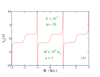
Figure 1: (Color online) Classical path $x^{(1)}_{cl}(\tau)$ in Eq. (17), for a choice of energy $E$ (in meV) and potential parameters: $a$ (in $\AA$), $\hbar\omega$ (in meV) and particle mass $M$ in units of the electron mass. The center of the (anti)instantons is taken at $\tau_{0}=\,0$.

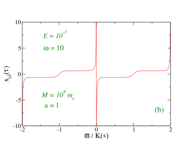
Figure 2: (Color online) Classical path $x^{(2)}_{cl}(\tau)$ in Eq. (17), for the same parameters as Fig. 1.

In fact such singularities, that remind us of the caustic points in the classical orbit of the harmonic oscillator schulman , happen to be outside the range physically relevant to our purposes. I clarify this point.

First, note that the solutions in Eq. (17) have a period $4K(s)$ thus, in principle, they should be discussed in the range $\varpi\in[-2K(s),2K(s)]$ since the amplitude $\theta$ of the elliptic integral varies as $\theta\in[-\pi,\pi]$. Second, focus on $x^{(1)}_{cl}(\tau)$ and apply the APBC, $x^{(1)}_{cl}(\tau=\,\pm L/2)=\,\pm a$, emboding the physics of the finite size problem. Setting $\tau_{0}=\,0$ without loss of generality, the first of Eq. (17) yields:

$$1=\,^{4}\sqrt{2\kappa}\,{}{{sn(\varpi^{*},s)dn(\varpi^{*},s)}\over{cn(\varpi^{*},s)}}\,$$

$$\varpi^{*}=\,\pm^{4}\sqrt{\kappa\over 2}{{\omega}}{L\over 2}$$ (18)

Representing the elliptic functions in Fourier series wang , I calculate Eq. (17) and obtain the values $\varpi^{*}$ fulfilling the APBC. Precisely, the computational method sets a value of $E$ and determines the corresponding $\varpi^{*}$ such as Eq. (18) holds. In this way the program calculates the period $L=\,L(E)$ and establishes the one to one correspondence between $E$ and $\omega^{*}$ at which the path interpolates between the minima. The ratio $\varpi^{*}/K(s)$ turns out to be always smaller than one, accordingly the singularities at $\varpi=\,\pm K(s)$ are physically avoided. In other words, the path $x^{(1)}_{cl}(\tau)$ always connects the potential minima well before encountering the singular points. Thus, taking the center of motion at $x_{cl}(\tau_{0}=\,0)=\,0$, $x^{(1)}_{cl}(\tau)$ properly describes a family of finite size (anti)instantons which are bounded, continuous and odd in the range $\tau\in[-L/2,L/2]$.

An analogous procedure with APBC applied to $x^{(2)}_{cl}(\tau)$ in Fig. 2 leads to determine the boundaries $\pm\varpi^{*}/K(s)$. As $\tau_{0}$ may be located everywhere along the $\tau-$ axis one may define in principle an even range $\varpi/K(s)$ with no singularities also for $x^{(2)}_{cl}(\tau)$. However, setting $\tau_{0}=\,0$, the choice of $x^{(1)}_{cl}(\tau)$ happens to be more convenient since the latter is well behaved for $\tau\in[-L/2,L/2]$.

The remarkable fact is that the $(\omega^{*},E)$ correspondences obtained by the two families of classical backgrounds are essentially identical. This means that the two independent solutions of the finite size classical equations of motion predict the same physics.

Correctly, in the limit $E\rightarrow 0\,\,\,(\kappa\rightarrow 1/2)$, one gets from Eq. (17):

$$x^{(1)}_{cl}(\tau)\rightarrow\,\pm a\tanh[\omega(\tau-\tau_{0})/\sqrt{2}]\,$$

$$x^{(2)}_{cl}(\tau)\rightarrow\,\mp a\coth[\omega(\tau-\tau_{0})/\sqrt{2}]$$ (19)

The first in Eq. (19) is the (anti)kink whose center of motion is set at $x^{(1)}_{cl}(\tau_{0})=\,0$ whereas the second is the solution of the infinite size classical equation Eq. (2) fulfilling the condition $x^{(2)}_{cl}(\tau_{0})=\,\infty$.

Further, using the relations:

$${{d\,{}sn(\varpi,s)}\over{d\varpi}}=\,cn(\varpi,s)dn(\varpi,s)\,$$

$${{d\,{}cn(\varpi,s)}\over{d\varpi}}=\,-sn(\varpi,s)dn(\varpi,s)\,$$

$${{d\,{}dn(\varpi,s)}\over{d\varpi}}=\,-s^{2}sn(\varpi,s)cn(\varpi,s)$$ (20)

one gets, from the first in Eq. (17), the particle path velocity as:

$${{\dot{x}_{cl}(\tau)}}=\,a\omega\sqrt{\kappa}\Biggl{[}1-2s^{2}sn^{2}(\varpi,s)+{{sn^{2}(\varpi,s)dn^{2}(\varpi,s)}\over{cn^{2}(\varpi,s)}}\Biggr{]}\,$$

(21)

Using the second of Eq. (15), one can easily check that Eq. (21) does not vanish on the $\tau$-range boundaries consistently with the general constraint expressed by Eq. (9). The latter, together with Eq. (21), permits to define the one to one correspondence between $E$ and $\omega^{*}$.

3. Semiclassical Path Integral

In the semiclassical model, the particle path $x(\tau)$ splits in the classical background $x_{cl}(\tau)$ plus the quantum fluctuations $\eta(\tau)$. Thus, the path integral for space-time particle propagation between the positions $x_{i}$ and $x_{f}$ in an imaginary time $L$ is:

$$<x_{f}|x_{i}>_{L}=\,\exp\biggl{[}-{{A[x_{cl}}\over{\hbar}}\biggr{]}\cdot\int D\eta(\tau)\exp\biggl{[}-{{A_{f}[\eta]}\over{\hbar}}\biggr{]}\,$$

(22)

The classical action $A[x_{cl}]$ is formally given by

$$A[x_{cl}]=\,\sqrt{2M}\int_{-a}^{a}dx_{cl}\sqrt{E+V(x_{cl})}-E\cdot L(E)\,$$

(23)

Inserting the potential in Eq. (1), Eq. (23) transforms into:

$$A[x_{cl}]=\,A_{0}\int_{0}^{1}dy\sqrt{{{4E}\over{\delta a^{4}}}+(1+y)^{2}(1-y)^{2}}-E\cdot L(E)\,$$

$$A_{0}=\,{{\sqrt{2}\delta a^{4}}\over\omega}$$ (24)

suitable for computation while, in the limit $E\rightarrow 0$, one obtains the well known result:

$$A[x_{cl}] \rightarrow \,{{2\sqrt{2}}\over 3}{{M^{2}\omega^{3}}\over\delta}$$ (25)

Eq. (25) represents the (anti)kink energy (in units of $\hbar$) whose inverse dependence on $\delta$ has been pointed out in the Introduction.

Being quadratic in the quantum fluctuations, $A_{f}[\eta]$ defines a stability equation whose eigenvalues represent the fluctuation spectrum kleinert . Carrying out Gaussian path integrals over the fluctuation paths, one gets formally

$$\int D\eta(\tau)\exp\biggl{[}-{1\over{\hbar}}A_{f}[\eta]\biggr{]}=\,\aleph\cdot Det\Bigl{[}\hat{O}\Bigr{]}^{-1/2}\,$$

$$\hat{O}\equiv-\partial_{\tau}^{2}+{{V^{\prime\prime}(x_{cl}(\tau))}/M}$$ (26)

where $\aleph$ depends on the measure of integration. The heart of the matter is the evaluation of the functional determinant in Eq. (26). Three observations permit to get the clue to the problem.

A) Differentiating Eq. (2) with respect to $\tau$, one notes that ${\dot{x}_{cl}(\tau)}$ solves the homogeneous equation associated to the second order Schrödinger-like differential operator $\hat{O}$

$$\hat{O}\eta(\tau)=\,0$$ (27)

As a general consequence of the $\tau$-translational invariance, a Goldstone mode appears in the system and this is true both for the infinite and the finite size cases. Thus, the particle path velocity is proportional to the fluctuation which makes $A_{f}[\eta]$ vanishing, ${\dot{x}_{cl}(\tau)}\propto\eta_{0}(\tau)$ with eigenvalue $\varepsilon_{0}=\,0$.

B) As ${{x}_{cl}(\tau)}$ is monotonic within a period $L$, ${\dot{x}_{cl}(\tau)}$ has no nodes hence, $\eta_{0}(\tau)$ represents the ground state and $\varepsilon_{0}$ is the lowest eigenvalue in the fluctuation spectrum in agreement with the fact that the potential is stable. However, the zero mode eigenvalue breaks the Gaussian approximation and makes the path integral divergent. The trouble is overcome by regularizing the fluctuations determinant, extracting $\varepsilon_{0}$ from Eq. (26) and evaluating its contribution separately resorting to collective coordinates langer ; kleinert . The replacement yields, for the infinite and finite size theories respectively:

$$(\varepsilon_{0})^{-1/2}\rightarrow\,\sqrt{{{A[x_{cl}]}\over{2\pi\hbar}}}L\,{}\,\,\,\,\,{infinite\,\,\,size}\,$$

$$(\varepsilon_{0})^{-1/2}\rightarrow\,\sqrt{{{A[x_{cl}]+E\cdot L}\over{2\pi\hbar}}}L\,{}\,\,\,\,\,{finite\,\,\,size}\,$$

(28)

Note incidentally that also the infinite size instantonic theory assumes, strictly speaking, that the size $L$ along the $\tau-$ axis is finite (although large) so that $\varepsilon_{0}^{-1/2}\propto L$ and the path integral is finite. Otherwise the zero mode singularity could not be removed. This observation points to a formal contradiction of the infinite size theory that, in fact, stimulated me to develop a consistent description in which both the classical background and the zero mode of the quantum fluctuations can be precisely determined at any finite size.

C) As stated below Eq. (21), $\dot{x}_{cl}(\tau)$ takes the same values on the $\tau-$ boundaries. More generally, for any two points $\varpi_{1},\varpi_{2}$ such that $\varpi_{2}=\,\varpi_{1}\pm 2K(s)$, from Eq. (21) one gets: $\dot{x}_{cl}(\varpi_{2})=\,\dot{x}_{cl}(\varpi_{1})$. As the path velocity is (proportional to) the ground state fluctuation, the important consequence is that the fluctuation eigenmodes obey periodic boundary conditions (PBC).

Collecting the informations from A) to C) and using a fundamental result of the theory of functional determinants with PBC forman , I rewrite the fluctuation determinant in Eq. (26) as

$$Det[\hat{O}]=\,\varepsilon_{0}\cdot Det^{R}[\hat{O}]\,$$

$$Det^{R}[\hat{O}]=\,{{<\eta_{0}|\eta_{0}>\bigl{(}\eta_{1}(\varpi_{2})-\eta_{1}(\varpi_{1})\bigr{)}}\over{{\eta_{0}(\varpi_{1})W(\eta_{0},\eta_{1})}}}$$ (29)

Where $Det^{R}[\hat{O}]$ indicates that the determinant is regularized mckane after extracting the zero eigenvalue. $\eta_{0}$ and $\eta_{1}$ are independent solutions of Eq. (27):

$$\eta_{0}=\,\dot{x}_{cl}\,$$

$$\eta_{1}=\,{{\partial{x}_{cl}}\over{\partial m}};\,{}\,m=\,s^{2}$$ (30)

$W(\eta_{0},\eta_{1})$ is their Wronskian and $<\eta_{0}|\eta_{0}>$ is the squared norm. Using the first in Eq. (17) and Eq. (30), $Det^{R}[\hat{O}]$ can be worked out analytically.

4. Regularized Fluctuation Determinant

I show now in detail how to obtain the regularized $Det^{R}[\hat{O}]$ of Eq. (29) on the base of the Wronskian construction. The two points $\varpi_{2},\varpi_{1}$ map onto $L/2$ and $-L/2$ along the $\tau-$ axis according to the definition in Eq. (15).

I) The $\tau-$ derivatives of the two independent solutions $\eta_{0}$ and $\eta_{1}$ of Eq. (30) read respectively:

$$\dot{\eta}_{0}(\tau)=\,{\ddot{x}_{cl}(\tau)}\,$$

$$\dot{\eta}_{1}(\tau)=\,{\partial\over{\partial m}}\Bigl{[}{{\partial{x}_{cl}(\tau)}\over{\partial\varpi}}\cdot{{\partial\varpi}\over{\partial\tau}}\Bigr{]}$$ (31)

Then, the Wronskian $W(\eta_{0},\eta_{1})$ is:

$$W(\eta_{0},\eta_{1})=\,\dot{x}_{cl}(\tau){{\partial\dot{x}_{cl}(\tau)}\over{\partial m}}-{\ddot{x}_{cl}(\tau)}{{\partial{x}_{cl}(\tau)}\over{\partial m}}\,$$

(32)

The Wronskian is constant and therefore can be calculated in any convenient $\tau\in[-L/2,L/2]$. The center of the classical paths, located at $\tau_{0}$, is the best choice as $\ddot{x}_{cl}(\tau_{0})\equiv\,{{x}_{cl}(\tau_{0})=\,0}$ and $\dot{x}_{cl}(\tau_{0})=\,a\omega\sqrt{\kappa}$.

Observing that:

$${{\partial\varpi}\over{\partial\tau}}=\,{{\omega}\over{2\sqrt{s^{2}-1/2}}}\,$$

$${\partial\over{\partial m}}\Bigl{[}{{\partial\varpi}\over{\partial\tau}}\Bigr{]}=\,-{\omega\over 4}(s^{2}-1/2)^{-3/2}\,$$

(33)

from Eqs. (31) and  (32), I get

$$W(\eta_{0},\eta_{1})=\,-{{\omega^{2}a^{2}}\over{16}}(s^{2}-1/2)^{-3}$$ (34)

II) I evaluate $\eta_{1}(\tau=\,\pm L/2)$ writing $\eta_{1}$ as

$$\eta_{1}(\tau)=\,{{\partial{x}_{c}(\tau)}\over{\partial\varpi}}\cdot{{\partial\varpi}\over{\partial m}}\,$$

$$\varpi=\,{1\over 2}F(\theta,s)$$ (35)

Using the relations:

$${{\partial\varpi}\over{\partial m}}=\,{1\over{4s}}{{\partial F(\theta,s)}\over{\partial s}}\,$$

$${{\partial F(\theta,s)}\over{\partial s}}=\,{s\over{\bar{s}^{2}}}\Biggl{[}{{E(\theta,s)-\bar{s}^{2}F(\theta,s)}\over{s^{2}}}-{{\sin\theta\cos\theta}\over{\sqrt{1-s^{2}\sin^{2}\theta}}}\Biggr{]}\,$$

$$E(\theta,s)=\,\int_{0}^{\theta}{{d\alpha}{\sqrt{1-s^{2}\sin^{2}\alpha}}}\,$$

$$\bar{s}^{2}=\,1-s^{2}$$ (36)

I derive the following boundary properties:

$$\theta(L/2)=\,2arctan\Biggl{(}{1\over{\,{}^{4}\sqrt{2\kappa}}}\Biggr{)}=\,-\theta(-L/2)\,$$

$$F\bigl{(}\theta(L/2),s\bigr{)}=\,-F\bigl{(}\theta(-L/2),s\bigr{)}\,$$

$$E\bigl{(}\theta(L/2),s\bigr{)}=\,-E\bigl{(}\theta(-L/2),s\bigr{)}\,$$

(37)

After setting $\tau_{0}=\,0$, it follows that:

$$\eta_{1}(L/2)=\,-\eta_{1}(-L/2)\,$$

$$\eta_{1}(-L/2)=\,\dot{x}_{c}(-L/2)\Bigl{[}\biggl{(}{{\partial\varpi}\over{\partial\tau}}\biggr{)}^{-1}\cdot{{\partial\varpi}\over{\partial m}}\Bigr{]}_{\tau=\,-L/2}\,$$

$$\dot{x}_{c}(\pm L/2)=\,2a\omega\sqrt{\kappa}\,s^{2}\bigl{(}1-sn^{2}(\varpi^{*})\bigr{)}\,$$

$$sn^{2}(\varpi^{*})=\,{{1-\cos[\theta(L/2)]}\over{1+\sqrt{1-s^{2}\sin^{2}[\theta(L/2)]}}}\,$$

$$\varpi^{*}=\,\pm{{\omega L}\over{4\sqrt{s^{2}-1/2}}}$$ (38)

The last in Eq. (38) coincides with $\varpi^{*}$ in Eq. (18). Note that $\eta_{1}$ is a solution of Eq. (27) but, unlike $\eta_{0}$, it does not represent a quantum fluctuation component. This explains why $\eta_{1}$ is odd on the boundaries whereas $\eta_{0}$ fulfills PBC. Thus, $Det^{R}[\hat{O}]$ in Eq. (29) can be rewritten as:

$$Det^{R}[\hat{O}]=\,{2{{<\eta_{0}|\eta_{0}>}\over{W(\eta_{0},\eta_{1})}}}\Bigl{(}{{\partial\varpi}\over{\partial\tau}}\Bigr{)}^{-1}{{\partial\varpi}\over{\partial m}}\Bigl{|}_{\tau=\,L/2}\,$$

(39)

The last factor in Eq. (39) is computed via Eqs. (36), (37) and turns out to be positive thus ensuring the correct (negative) sign to $Det^{R}[\hat{O}]$ (due to $W(\eta_{0},\eta_{1})<\,0$). It is well known from the general theory that only ratios of functional determinants have physical meaning both in value and sign. In fact being a product of an infinite number of eigenvalues with modulus larger than one, each determinant is separately divergent in the $L\rightarrow\infty$ limit. To get a finite ratio, I normalize $Det^{R}[\hat{O}]$ over the harmonic oscillator determinant $Det[\hat{h}]$ which, for periodic boundary conditions, reads:

$$Det[\hat{h}]=\,-4\sinh^{2}(\omega L/2)\,$$

$$\hat{h}\equiv\,-\partial^{2}_{\tau}+\omega^{2}$$ (40)

As $Det[\hat{h}]$ and $Det^{R}[\hat{O}]$ have the same exponential divergence, their ratio is finite in the $L\rightarrow\infty$ limit. Moreover it is positive, consistently with the fact that the contribution by the zero mode eigenvalue (extracted from $Det[\hat{O}]$) is positive. Therefore also $Det[\hat{O}]/Det[\hat{h}]$ has to be positive since the system is stable and there are no lower eigenvalues below the zero mode eigenvalue.

III) $\eta_{0}$ is proportional to the ground state ortonormal component in the series expansion for the path fluctuation. I define $\bar{\eta}_{0}=\,\bar{N}\eta_{0}$ such that, in Eq. (39), $<\eta_{0}|\eta_{0}>\equiv\,\bar{N}^{-2}$. Then, using Eq. (21), I derive the squared norm in the form

$$\bar{N}^{-2} = \,G\int_{0}^{\varpi^{*}}d\varpi\Biggl{[}1-2s^{2}sn^{2}(\varpi,s)+{{sn^{2}(\varpi,s)dn^{2}(\varpi,s)}\over{cn^{2}(\varpi,s)}}\Biggr{]}^{2}\,$$

$$G = \,{{\omega a^{2}}\over{2(s^{2}-1/2)^{3/2}}}$$ (41)

suitable for computation. Alternatively, one may proceed through the definition of the classical action in Eq. (23) and get:

$$\bar{N}^{-2}=\,{1\over M}\Bigl{(}{{A[x_{cl}]}}+{E\cdot L(E)}\Bigr{)}$$ (42)

In any case $<\eta_{0}|\eta_{0}>$ has the dimension of $[\omega a^{2}]$ hence, from Eqs. (33), (34), (41), it follows that $Det^{R}[\hat{O}]$ is proportional to $\omega^{-2}$ and correctly it does not carry any dependence on $a$. This completes the analysis since all ingredients required to compute Eq. (39) are now known.

Taking the ratio between the determinants in Eq. (39) and Eq. (40), in the $L\rightarrow\infty$ limit, I get

$${{Det^{R}[\hat{O}]}\over{Det[\hat{h}]}}\rightarrow{1\over{12\omega^{2}}}$$ (43)

thus recovering the well known value of the infinite size instantonic approach. This proves the correctness of the analytical procedure.

Then, the semiclassical path integral in Eq. (22) for one (anti)instanton takes the final expression:

$$<x_{f}|x_{i}>_{L}=\,\sqrt{{M\over{2\pi\hbar L}}}\cdot{1\over{2\sinh\bigl{(}\omega L/{2}\bigr{)}}}\Omega(L)L\,$$

$$\Omega(L)=\,\exp\biggl{[}-{{A[x_{cl}]}\over{\hbar}}\biggr{]}\cdot\Omega^{QF}(L)\,$$

$$\Omega^{QF}(L)=\,\sqrt{{{M\bar{N}^{-2}}\over{2\pi\hbar}}}\sqrt{{{Det[\hat{h}]}\over{Det^{R}[\hat{O}]}}}$$ (44)

which can be evaluated using Eq. (24), (39), (40), (42). Note that: i) The harmonic determinant is, in turn, normalized over the free particle determinant $Det[-\partial^{2}_{\tau}]=\,\sqrt{{M\over{2\pi\hbar L}}}$ which incorporates the constant $\aleph$. ii) $\Omega^{QF}(L)$ accounts for the quantum fluctuation effects in the finite size tunneling problem. iii) $\Omega(L)$ is the overall tunneling frequency which removes the twofold degeneracy of the double well potential in a finite domain. From the path integral in Eq. (44) one can extract the physical properties of the closed quantum system.

5. Final Remarks

This work presents the mathematical description of the finite size semiclassical theory for the bistable $\phi^{4}$ potential based on the Euclidean path integral formalism. In particular the two key ingredients of the model, namely classical equation of motion and quantum fluctuation spectrum, are analysed in detail. I have studied the classical equation of motion and obtained the family of classical paths which interpolates between the potential minima in the finite size system: such paths are necessarily associated to positive classical energies and fulfill antiperiodic boundary conditions. Around such non trivial background one may derive the mass spectrum in $\phi^{4}$ theories toharia by solving a stability equation more general than the standard Lamè equation associated to Eq. (8) harrin .

Due to the time translational invariance, the spectrum of the quadratic quantum fluctuations contains a zero mode which breaks the Gaussian approximation and makes the path integral divergent. The result of the regularization procedure for the finite size case is presented. Using the theory of the functional determinants, I have derived the regularized fluctuations determinant giving the full set of equation required to compute it. Finally, I have evaluated the contribution to the path integral originating from the quantum fluctuations and obtained an explicit expression for the tunneling energy in the finite size bistable $\phi^{4}$ model. This study permits to compute, for specific choices of potential parameters, the finite size induced renormalization of the tunneling energy with respect to the predictions of the infinite size instantonic approach. In view of the mapping to the temperature axis allowed by the Matsubara formalism, the obtained results may be well applied to calculate, for instance, the thermodynamical properties of systems described by Ginzburg-Landau field theories krum ; zinn , the finite $T$ splitting energy in two level systems arising in amorphous compounds zawa ; io3 and materials with local structural instabilities yuand ; io4 ; io5 as well as in solids showing macroscopic quantum tunneling of magnetization stampchud .

Along similar semiclassical patterns one can study a metastable $\phi^{4}$ model in finite size. For the latter one has to build the generalized bounce solution (whose properties however differ very much from those of the instanton) and analyse the quantum fluctuation spectrum with particular care to the ground state negative eigenvalue which causes metastability. The softening of the low lying fluctuation modes together with the decay rate for a finite size system will be the subject of a next work.

References

- (1) L.D.Landau, E.M.Lifshitz, Quantum Mechanics 3rd Edition, Butterworth-Heinemann, Oxford (1977).
- (2) M.V.Berry, K.E.Mount, Rep. Prog. Phys. 35, 315 (1972).
- (3) M.Zoli, Phys. Rev. B 72, 214302 (2005).
- (4) S.Coleman, Phys. Rev. D 15, 2929 (1977); C.G.Callan, S.Coleman, Phys. Rev. D 16, 1762 (1977).
- (5) J.S.Langer, Ann. Phys. 41, 108 (1967).
- (6) C.M.Bender and T.T.Wu, Phys. Rev. Lett. 21, 406 (1968); ibid. Phys. Rev. 184, 1231 (1969).
- (7) B.Simon, Ann. Phys. 58, 76 (1970).
- (8) A.M.Sanchez and J.D.Bejarano, J.Phys.A: Math.Gen. 19, 887 (1986).
- (9) R.Dashen, B.Hasslacher and A.Neveu, Phys. Rev. D 10, 4114 (1974); ibid. 11, 3424 (1975); ibid. 12, 2443 (1975).
- (10) A.Garg, Am.J.Phys. 68, 430 (2000).
- (11) M.Lüscher, Commun. Math. Phys. 104, 177 (1986).
- (12) G.Mussardo, V.Riva and G.Sotkov, Nucl. Phys. B 670, 464 (2003).
- (13) G.Plunien, B.Müller, W.Greiner, Phys. Rep. 134, 87 (1986).
- (14) K.Langfeld, F.Schmüser, H.Reinhardt, Phys. Rev. D 51, 765 (1995).
- (15) J.Garcia-Ojalvo, J.M.Sancho, Noise in Spatially Extended Systems, Springer, N.Y./Berlin (1999).
- (16) W.G.Faris and G.Jona-Lasinio, J.Phys.A 15, 3025 (1982).
- (17) H.-B.Braun, Phys. Rev. Lett. 71, 3557 (1993).
- (18) A.I.Yanson, I.K.Yanson and J.M. van Ruitenbeck, Nature 400, 144 (1999); ibid. Phys. Rev. Lett. 84, 5832 (2000).
- (19) A.Zamolodchikov, J.Phys.A:Math.Gen. 39, 12863 (2006).
- (20) R.P.Feynman, Rev. Mod. Phys. 20, 367 (1948).
- (21) R.P.Feynman and A.R.Hibbs, Quantum Mechanics and Path Integrals Mc Graw-Hill, New York (1965).
- (22) I.M.Gelfand and A.M.Yaglom, J.Math.Phys. 1, 48 (1960).
- (23) R.Forman, Invent.Math. 88, 447 (1987).
- (24) A.J.McKane and M.B.Tarlie, J.Math.Phys. 28 (1995) 6931.
- (25) H.Kleinert, Path Integrals in Quantum Mechanics, Statistics, Polymer Physycs and Financial Markets, World Scientific Publishing, Singapore (2004).
- (26) R.Rajaraman, Solitons and Instantons North Holland, Amsterdam (1982).
- (27) T.Schäfer and E.V.Shuryak, Rev.Mod.Phys. 70, 323 (1998).
- (28) J.-Q.Liang, H.J.W.Müller-Kirsten, D.K.Park and F.Zimmerschied Phys. Rev. Lett. 81, 216 (1998).
- (29) J.Ankerhold and H.Grabert, Phys. Rev. E 61, 3450 (2000).
- (30) R.S.Maier and D.L.Stein, Phys. Rev. Lett. 87, 270601 (2001).
- (31) Z.X.Wang and D.R.Guo, Special Functions, World Scientific, Singapore (1989).
- (32) M.Abramowitz and I.A.Stegun, Handbook of Mathematical Functions, Dover Publications, New York (1972).
- (33) L.S.Schulman, Techniques and Applications of Path Integration, Wiley&Sons, New York (1981).
- (34) B.Grzadkowski, M.Toharia, CERN-PH-TH/2004-003
- (35) B.J.Harrington, Phys. Rev. D 18, 2982 (1978).
- (36) J.A.Krumhansl, J.R.Schrieffer, Phys. Rev. B 11, 3535 (1975).
- (37) J. Zinn-Justin, Quantum Field Theory and Critical Phenomena Clarendon Press, Oxford (1989).
- (38) K.Vladár, A.Zawadowski, Phys. Rev. B 28, 1564 (1983); ibid. 28, 1582 (1983); ibid. 28, 1596 (1983).
- (39) M.Zoli, Acta Physica Polonica A 77, 639 (1990).
- (40) C.C.Yu, P.W.Anderson, Phys.Rev.B 29, 6165 (1984).
- (41) M.Zoli, Phys.Rev.B 44, R7163 (1991).
- (42) M.Zoli, in Lattice Effects in High Superconductors, eds. Y.Bar-Yam, T.Egami, J.Mustre de Leon, A.R.Bishop. World Scientific, Singapore (1992) p.195.
- (43) P.C.E.Stamp, E.M.Chudnovsky, B.Barbara, Int. J. Mod. Phys.B 6, 1355 (1992).