Abstract

All elementary Hamiltonians in nature are expected to be invariant under rotation. Despite this restriction, we usually assume that any arbitrary measurement or unitary time evolution can be implemented on a physical system, an assumption whose validity is not obvious. We introduce two different schemes by which any arbitrary time evolution and measurement can be implemented with desired accuracy by using rotationally invariant Hamiltonians that act on the given system and two ancillary systems serving as reference frames. These frames specify the $z$ and $x$ directions and are independent of the desired time evolution. We also investigate the effects of quantum fluctuations that inevitably arise due to usage of a finite system as a reference frame and estimate how fast these fluctuations tend to zero when the size of the reference frame tends to infinity. Moreover we prove that for a general symmetry any symmetric quantum operations can be implemented just by using symmetric interactions and ancillas in the symmetric states.

PACS numbers:

Typeset Using LaTeX

1 Introduction

In describing any physical system a reference frame is indispensable. The state of a system is not an abstract concept independent of a reference frame; the only meaningful and measurable observables are correlations between the main physical system and a reference frame. A reference frame itself is always represented with a physical system. In practice we do not consider reference frames as quantum systems, and we treat them classically. However there are theoretical considerations that force us to treat reference frames quantum mechanically. This can be regarded as the counterpart of the famous idea that information is physical: since information is stored in the state of some physical object that is subject to the laws of physics, at the most fundamental level the abilities and limitations of these physical objects for information processing depends on these physical laws. In the same way, a reference frame is always carried by a physical system. Indeed, it has been argued that the various conceptual conundrums in quantum mechanics – such as controversies about existence of superposition between number states in quantum optics, superconductivity and Bose-Einstein condensation, or the problem of quantification of entanglement in systems of bosons and fermions [1] – are rooted in ignoring the role of reference frames.

Amongst the variety of reasons for considering reference frames as quantum mechanical objects, we are interested in the following. First, all elementary interactions in nature are expected to have specific symmetries. For example, they do not have a preferred direction and so are rotationally invariant. Given this situation, a question arises as to whether or not it is possible to implement an arbitrary Hamiltonian and measurements that might not have that symmetry. The problem of restrictions on quantum operations imposed by assuming a given symmetry was first emphasized by Wigner [2]. Assuming all Hamiltonians commute with some symmetry operator, he showed that it is impossible to measure an observable that does not commute with that symmetry operator. Later Araki and Yanase [3] proposed a scheme to measure an operator that does not commute with that symmetry operator to any desired accuracy. To this end they used a quantum system acting as a reference frame beside the main system. The accuracy of that measurement increases with the size of the Hilbert space of that reference frame (though not necessarily linearly).

The second reason for treating reference frames as quantum mechanical objects, which is related to the first one, arises from the aspiration to have a relational quantum mechanics [4, 5]. By relational we mean a theory in which we do not have an external reference frame that is used to define kinematical observables. The key motivator here is general relativity, a background independent theory whose quantum generalization is also expected to inherit this property. In the semi-classical limit, where reference frames are assumed to have a large Hilbert space, relational quantum mechanics reduces to standard quantum mechanics. However at the semi-classical limit we cannot neglect gravitational effects due to these reference frames [4, 5, 6, 7]. So the problem of finding “relational quantum mechanics” is necessarily part of the project of constructing a quantum theory of gravity.

There are other situations that force us to treat reference frames as quantum mechanical objects. Specifically, in quantum computation we need to perform measurements on a small quantum register. In this case the quantum register must be strongly coupled to the apparatus. This requirement forces usage of small and cold apparatus [8]. For example, in some proposed experiments for measuring spin, a small magnet is used to measure a single spin. Note that this magnet can be considered as the reference frame that defines a specific direction. Due to its small size, the magnet should be treated as a quantum mechanical object [9, 10] .

Considering a bounded quantum mechanical object as a reference frame has some side effects. First of all, using a bounded quantum reference frame we cannot implement the measurement or time evolution perfectly. There are inevitably quantum mechanical fluctuations [1, 6, 11]. Second, performing a measurement or a time evolution has always some back-reaction on the reference frame and degrades it [7, 8, 11].

We consider here the problem of implementing any arbitrary unitary transformation on a physical system. We show that this can be accomplished using two ancillary systems that act as two reference frames, referred to as X-RF and Z-RF, respectively specifying the x and z directions. Note that the state of the reference frame is independent of the desired unitary transformation. As the dimension of the Hilbert space of both reference frames tends to infinity, the implemented operation becomes the same as the desired one. We first construct a primary scheme in which, by using an isotropic unitary transformation and a reference frame Z-RF, we can implement all unitary operations on the system that commute with $L_{Z}$. We then use this to construct two different schemes, scheme I and scheme II , each of which ensures that our desired unitary transformation is implemented to a given accuracy. In scheme I we employ a unitary transformation commuting with $L_{Z}$ that acts on both the physical system and an auxiliary frame X-RF whose angular momentum is large. Changes in the angular momentum of the system that occur due to the implementation of this unitary transformation can be compensated by changes in the angular momentum of X-RF. In the scheme II we construct a sequence of unitary operators that alternately commute with $L_{Z}$ and $L_{X}$, and respectively make use of a sequence of Z-RFs and X-RFs, and show how any desired unitary transformation can be implemented via this sequence.

Any measurement consists of a process in which a measurement apparatus initially uncorrelated with a system of interest changes so that some property of the apparatus becomes correlated with some physical property of the system. As with all other quantum phenomena, this can be described by a unitary time evolution acting on the system and measurement apparatus. Therefore using this scheme we can implement any arbitrary measurement just using isotropic interactions; in this sense we can regard this work as a kind of generalization of ref. [3]. Our work also generalizes the simple model that Poulin [6] used to show how it is possible to construct relational quantum mechanics from ordinary quantum mechanics using some specific rules. In that toy model a reference frame specifying the $z$ direction was constructed and used to measure the spin of a spin-1/2 particle.

Alternatively, this problem is closely related to the issue of restrictions imposed by superselection rules. Originally these rules were regarded as some axiomatic limitations added to the theory that restrict the set of physically realizable operations [12]. For example the superselection rule for electric charge forbids the production of superposed states with different charges. On the other hand, as emphasized more recently [1], the lack of a reference frame breaking some symmetry imposes restrictions on implementable operations, which can can be regarded as superselection rules. For example, assuming all interactions are rotationally invariant, without any reference frame that breaks this symmetry, we cannot prepare states that are not rotationally invariant; we also cannot perform time evolutions and measurements that are not rotationally invariant. In this way the latter superselection rules might seem more fundamental. However as first argued by Aharanov and Susskind [13, 14], emergence of those fundamental superselection rules in non-relativistic quantum theory results from making the (unphysical) assumption that there exist absolute operations without any dependence on some quantum reference frame. In ref. [15] Kitaev et al. showed that all superselection rules described by compact groups result from the lack of an appropriate reference frame. In their terminology, an invariant world, which is subject to a superselection rule described by a compact Lie group by virtue of an unbounded quantum reference frame (which itself is subject to those superselection rules) can simulate the physics of an unrestricted world that is not subject to those superselection rules. To show this, they prove that for all states, time evolutions, and measurements on a particular system in the unrestricted world there exist states, time evolutions and measurements associated with the total system, including that particular system and quantum reference frame, that are invariant under the group describing those superselection rules. Moreover they produce the same observable effects. Then using this fact they show that superselection rules do not enhance the information-theoretic security of quantum cryptographic protocols.

However, our work is distinct from ref. [15] in that we wish to perform an arbitrary time evolution or measurement on some given unknown arbitrary state of a physical system; we do not want to simulate that physics, but we want to exactly perform unrestricted operations using a quantum reference frame which breaks that symmetry. We therefore assume that the initial states of the system and quantum reference frame are uncorrelated. However in the scheme proposed by Kitaev et al [15], to a state of the system in the unrestricted world they associate an initial state in the invariant world that is not necessarily the tensor product of that initial state of the system and a state of the reference frame. Indeed, the only case in which this initial state is a tensor product is just the trivial case where the initial state of the system is invariant under that group. Hence given some unknown arbitrary state of the system, using their scheme we cannot perform all quantum operations.

The preceding discussion was concerned with cases in which implementation of non-symmetric time evolution requires non-symmetric resources, i.e. a reference frame that breaks the symmetry. However it is usually implicitly assumed that to implement a symmetric quantum operation one needs no non-symmetric resources. In the other words, the assumption is that any symmetric quantum operation can be realized by a symmetric unitary evolution acting on the system and an ancillary system in a symmetric state. Before working more on the non-symmetric cases we check the validity of this assumption in the next section. For a general compact symmetry group, and any given symmetric quantum operation we find an explicit form of a symmetric unitary time evolution acting on the system and a symmetric ancilla that realize the given quantum operation.[17]

In this paper we denote by $R$-inv a rotationally invariant quantity, and $Z$-inv,$X$-inv for unitary operators that are invariant under rotation around the $Z$ and $X$ axes respectively.

The outline of our paper is as follows. In section 2 we show that only symmetric resources are required to carry out any given symmetric quantum operation. Then in section 3 we introduce a distance measure for quantum operations and investigate some of its useful properties. In section 4 we discuss how to classify unitary operators with rotational symmetry, both in general and about one axis. We discuss in section 5 how to implement $Z$-inv unitary operators using $R$-inv (ie fully rotationally invariant) operators. In section 6 we show how to use $Z$-inv unitaries to implement all unitary operations, and then in the next two sections we respectively describe each of schemes I and II. We close in section 9 by comparing the two schemes from the point of view of the resources they require and with some suggestions for further research.

2 When are non-symmetric resources necessary?

Suppose a unitary time evolution with a specific symmetry acts on the main system and an ancillary system. We assume the initial state of ancillary system is also invariant under the symmetry. It is easy to see that the total effect of this time evolution on the system is described by a quantum operation that is invariant under the symmetry. Clearly if we make use only of symmetric resources, i.e. symmetric time evolutions and symmetric initial states, we obtain a symmetric quantum operation.

Consider next the inverse problem: is it possible to implement any given symmetric quantum operation using only symmetric resources, i.e. with a symmetric unitary time evolution and with an ancillary system which initially is in a symmetric state. As we might guess intuitively the answer is yes as we shall now demonstrate.

Consider a quantum operation $\varepsilon$ that is invariant under some group described by $G$. We call it a $G$-inv quantum operation. Our aim is to show that for any group $G$ and for any given $G$-inv quantum operation there exists a $G$-inv unitary time evolution $\mathscr{S}$ acting on the system and ancilla such that

$$\varepsilon(\rho)=tr_{anc}(\mathscr{S}(\rho\otimes\mathopen{|}0\mathclose{\rangle}\mathopen{\langle}0\mathclose{|})\mathscr{S}^{\dagger})$$ (2.1)

where $\mathopen{|}0\mathclose{\rangle}$, the initial state of the ancilla, is also $G$-inv. We prove this fact and give an explicit form of such a unitary time evolution [17].

We begin by noting that it has been shown [18] that a $G$-inv quantum operation always admits a Kraus decomposition with Kraus operators $K_{jm\alpha}$, where $j$ denotes an irrep, $m$ a basis for the irrep, and $\alpha$ a multiplicity index, satisfying

$$T(g)K_{jm\alpha}T^{\dagger}(g)=\sum_{m^{\prime}}u^{(j)}_{m^{\prime}m}(g)K_{jm^{\prime}\alpha}\ \ \forall g\in G$$ (2.2)

where $T(g)$ is the unitary operator in the Hilbert space of the system representing the effect of $g\in G$ on the state of system and $u^{(j)}$ is an irreducible unitary representation of $G$. We define $\mathopen{|}j,n,\alpha\mathclose{\rangle}$ a basis in which ${u}^{(j)}(g)$ has the following form.

$$T(g)\mathopen{|}j,n,\alpha\mathclose{\rangle}={u}^{(j)}(g)\mathopen{|}{j,n,\alpha}\mathclose{\rangle}=\sum_{n^{\prime}}{u}^{(j)}_{n^{\prime}n}(g)\mathopen{|}{j,n^{\prime},\alpha}\mathclose{\rangle}$$ (2.3)

On the other hand, if $u^{(j)}$ is a representation of $G$, then complex conjugate of $u^{(j)}$ in any specific basis is also a representation of $G$ which might be equivalent to $u^{(j)}$. We denote the representation obtained by complex conjugate of ${u}^{(j)}(g)$ in the basis $\mathopen{|}j,n,\alpha\mathclose{\rangle}$ by $\overline{u}^{(j)}$. There exists a basis $\mathopen{|}\overline{j,n,\alpha}\mathclose{\rangle}$ such that

$$T(g)\mathopen{|}\overline{j,n,\alpha}\mathclose{\rangle}=\overline{u}^{(j)}(g)\mathopen{|}\overline{j,n,\alpha}\mathclose{\rangle}=\sum_{n^{\prime}}\overline{u}^{(j)}_{n^{\prime}n}(g)\mathopen{|}\overline{j,n^{\prime},\alpha}\mathclose{\rangle}$$ (2.4)

To purify $\varepsilon$ we assume we have an ancillary system initially in the $G$-inv state $\mathopen{|}0\mathclose{\rangle}$ as in eq. (2.1) . We want to build a $G$-inv unitary $\mathscr{S}$ acting on the system and an ancillary system such that the effect of this unitary time evolution on the system is described by $\varepsilon$. Assume $\mathopen{|}\psi\mathclose{\rangle}$ is an arbitrary state of system. We define $P_{0}$ to be the subspace spanned by all states of the form of $\mathopen{|}\psi\mathclose{\rangle}\mathopen{|}0\mathclose{\rangle}$. Also we define $P_{1}$ to be the subspace spanned by all states $S\mathopen{|}\psi\mathclose{\rangle}\mathopen{|}0\mathclose{\rangle}$ where $S$ is

$$S\mathopen{|}\psi\mathclose{\rangle}\mathopen{|}0\mathclose{\rangle}=\sum_{jm\alpha}K_{jm\alpha}\mathopen{|}\psi\mathclose{\rangle}\mathopen{|}\overline{j,m,\alpha}\mathclose{\rangle}$$ (2.5)

where $\mathopen{|}\overline{j,m,\alpha}\mathclose{\rangle}$ are states of ancillary system for which Eq.(2.4) holds. So by definition $S$ is a map from $P_{0}$ to $P_{1}$ .We assume $\mathopen{|}0\mathclose{\rangle}$ is chosen such that it is orthogonal to all states $\mathopen{|}\overline{j,m,\alpha}\mathclose{\rangle}$ appearing in Eq.(2.5). This is possible because the ancilla can always be taken to have any number of singlet representations, one of which can be taken to be $\mathopen{|}0\mathclose{\rangle}$. So obviously $P_{0}$ and $P_{1}$ are orthogonal to each other.

Using the normalization condition $\sum_{j,m,\alpha}K_{jm\alpha}^{\dagger}K_{jm\alpha}=I$ it is straightforward to see that this map preserves inner product. Moreover we can show that $S$ commutes with $G$. Using eqs. (2.2) and (2.4) we have

$$T(g)\otimes T(g)\ S\mathopen{|}\psi\mathclose{\rangle}\mathopen{|}0\mathclose{\rangle} = \sum_{jm\alpha}T(g)K_{jm\alpha}\mathopen{|}\psi\mathclose{\rangle}\otimes T(g)\mathopen{|}\overline{j,m,\alpha}\mathclose{\rangle}$$ (2.6)

$$= \sum_{jm\alpha}\sum_{m^{\prime}}u^{(j)}_{m^{\prime}m}(g)K_{jm^{\prime}\alpha}T(g)\mathopen{|}\psi\mathclose{\rangle}\otimes\sum_{n^{\prime}}\overline{u}^{(j)}_{n^{\prime}m}(g)\mathopen{|}\overline{j,n^{\prime},\alpha}\mathclose{\rangle}$$

and from the unitarity of $u^{(j)}$ we find

$$T(g)\otimes T(g)\ S\mathopen{|}\psi\mathclose{\rangle}\mathopen{|}0\mathclose{\rangle}=\sum_{jn\alpha}K_{jn\alpha}T(g)\mathopen{|}\psi\mathclose{\rangle}\otimes\mathopen{|}j,n,\alpha\mathclose{\rangle}$$ (2.7)

Therefore

$$(T(g)\otimes T(g))\ S\mathopen{|}\psi\mathclose{\rangle}\mathopen{|}0\mathclose{\rangle}=S(T(g)\otimes I)\mathopen{|}\psi\mathclose{\rangle}\mathopen{|}0\mathclose{\rangle}=S(T(g)\otimes T(g))\mathopen{|}\psi\mathclose{\rangle}\mathopen{|}0\mathclose{\rangle}$$ (2.8)

where in the last step we have used this fact that $\mathopen{|}0\mathclose{\rangle}$ is $G$-inv. So $S$ commutes with $G$. Note that $T(g)\otimes T(g)\ \mathopen{|}\psi\mathclose{\rangle}\mathopen{|}0\mathclose{\rangle}$ is still in $P_{0}$ and so $T(g)\otimes T(g)S\mathopen{|}\psi\mathclose{\rangle}\mathopen{|}0\mathclose{\rangle}$ is still in $P_{1}$.

Now we define $S^{-1}$ to be a map from $P_{1}$ to $P_{0}$ such that

$$S^{-1}\left(\sum_{jm\alpha}K_{jm\alpha}\mathopen{|}\psi\mathclose{\rangle}\mathopen{|}\overline{j,m,\alpha}\mathclose{\rangle}\right)=\mathopen{|}\psi\mathclose{\rangle}\mathopen{|}0\mathclose{\rangle}$$ (2.9)

By definition all states in $P_{1}$ are of the form $\sum_{jm\alpha}K_{jm\alpha}\mathopen{|}\psi\mathclose{\rangle}\mathopen{|}\overline{j,m,\alpha}\mathclose{\rangle}$ for some $\mathopen{|}\psi\mathclose{\rangle}$ and so $S^{-1}$ is defined for all states in $P_{1}$. Since $S$ preserves inner product so does $S^{-1}$. Also from Eq.(2.8) we can deduce that $S^{-1}$ commutes with $G$. We define the subspace $P_{2}$ to be the subspace of all states in the Hilbert space of system and ancillary system except those who live in $P_{0}$ and $P_{1}$. Finally we can define a $G$-inv unitary $\mathscr{S}$ in the following manner.

$$\mathopen{|}\Omega\mathclose{\rangle}\in P_{0} : \mathscr{S}\mathopen{|}\Omega\mathclose{\rangle}=S\mathopen{|}\Omega\mathclose{\rangle}$$

$$\mathopen{|}\Omega\mathclose{\rangle}\in P_{1} : \mathscr{S}\mathopen{|}\Omega\mathclose{\rangle}=S^{-1}\mathopen{|}\Omega\mathclose{\rangle}$$ (2.10)

$$\mathopen{|}\Omega\mathclose{\rangle}\in P_{2} : \mathscr{S}\mathopen{|}\Omega\mathclose{\rangle}=\mathopen{|}\Omega\mathclose{\rangle}$$

So $\mathscr{S}$ exchanges $P_{0}$ by $P_{1}$ and leave all states in $P_{2}$ unchanged. Obviously $\mathscr{S}$ is unitary and commutes with $G$. Also it is straightforward to check that it satisfies Eq.(2.1) and so its total effect on the system would be $\varepsilon$. This means that for any $G$-inv quantum operation one can find a $G$-inv unitary time evolution such that effect of this unitary on the system is described by this quantum operation.

In general if a quantum operation is described by $N$ independent Kraus operators, to implement it with a unitary time evolution we need an ancillary system with an $N$ dimensional Hilbert space. In the scheme proposed above for implementing a $G$-inv quantum operation described by $N$ independent Kraus operators, we need an $N+1$ dimensional ancillary. So we see that restricting to symmetric resources increase the minimum of size required ancillary system at most by one.

With the same kind of argument we can prove that any given $G$-inv density operator of system can be purified such that the total pure state is $G$-inv. By definition a $G$-inv density operator should commute with all members of this group.

Any unitary representation of a group $G$ allows a decomposition of the Hilbert space into charge sectors $\mathscr{H}_{j}$ where each charge sector carries an inequivalent representation $T_{j}$ of $G$.

$$\mathscr{H}=\bigoplus_{j}\mathscr{H}_{j}$$ (2.11)

Each of these sectors has $n(j)$ copies of the representation $j$. On each of these sectors the effect of the representation of $g\in G$, $T(g)$, can be factorized to the irreducible representation associated with $j$, $T_{j}(g)$, times an identity that acts on the multiplicity subsystem $I_{n(j)}$. Hence it can be written in the form $T_{j}(g)\otimes I_{n(j)}$. Each sector can be therefore be decomposed into virtual subsystems [19]

$$\mathscr{H}_{j}=\mathscr{M}_{j}\otimes\mathscr{N}_{j}$$ (2.12)

The effect of $T(g)$ on $\mathscr{M}_{j}$ is $T_{j}(g)$ and on $\mathscr{N}_{j}$ is trivial . So finally the representation $T(g)$ can be written in the form

$$T(g)=\bigoplus_{j}T_{j}(g)\otimes I_{n(j)}$$ (2.13)

We call $\mathscr{M}_{j}$’s gauge spaces and $\mathscr{N}_{j}$’s multiplicity spaces. In the language of quantum information $\mathscr{M}_{j}$ and $\mathscr{N}_{j}$ are called decoherence-full subsystems and noiseless .

Using Schur’s lemmas we can show that a $G$-inv density operator can always be written as

$$\rho_{G-inv}=\sum_{j}p_{j}\frac{I_{j}}{tr(I_{j})}\otimes\rho^{(j)}$$ (2.14)

where $j$ specifies different inequivalent irreps, $I_{j}$ is the identity operator on the gauge subsystem of each irrep, $\rho_{j}$ is a density operator acting on the multiplicity subsystem of each irrep, and $\{p_{j}\}$ is a probability distribution. Suppose $\mathopen{|}\phi^{(j)}\mathclose{\rangle}$, which is a purification of $\rho^{(j)}$, is expanded as follows:

$$\mathopen{|}\phi^{(j)}\mathclose{\rangle}=\sum_{\alpha,\beta}c^{(j)}_{\alpha,\beta}\mathopen{|}\alpha\mathclose{\rangle}\mathopen{|}\beta\mathclose{\rangle}\quad.$$

We can deduce that the following state is a $G$-inv purification of $\rho_{G-inv}$

$$\mathopen{|}\Delta\mathclose{\rangle}=\sum_{j,n}\sqrt{p_{j}}\mathopen{|}j,n\mathclose{\rangle}\otimes\mathopen{|}\overline{j,n}\mathclose{\rangle}\otimes\mathopen{|}\phi^{(j)}\mathclose{\rangle}=\sum_{j,n,\alpha,\beta}\sqrt{p_{j}}c^{(j)}_{\alpha,\beta}\mathopen{|}j,n,\alpha\mathclose{\rangle}\otimes\mathopen{|}\overline{j,n,\beta}\mathclose{\rangle}$$

where $\mathopen{|}j,n\mathclose{\rangle}$ and $\mathopen{|}\overline{j,n}\mathclose{\rangle}$ are respectivel vectors in the gauge subsystem of the main system and the ancillary one. With the same kind of argument we used in Eq.(2.6) we can see that this state is $G$-inv. As a simple example, we can check that for the case of $SU(2)$ as the symmetry group and the invariant density operator for spin half, which is $I/2$, the invariant purification state given by this method would be the singlet state.

Suppose Alice’s world is interacting and probably entangled with Bob’s world such that all of states and time evolution in her world have a specific symmetry. According to the above discussion she can never ascertain whether the whole world, including her system and Bob’s, has this same symmetry. On the other hand, if there existed quantum operations or mixed states that were not purifiable by symmetric resource, by observing those states or time evolutions she could ascertain that the whole world is not subject to that symmetry.

3 Distance between two quantum operations

To estimate the accuracy of implementing unitary time evolutions we need a measure to compare the implemented time evolution with the desired one. In this section we introduce a distance for comparing two quantum operations and investigate some of its main properties that we shall utilize in this paper.

Consider two quantum operations $\varepsilon_{1}$ and $\varepsilon_{2}$ that map density matrices to density matrices. By definition these are trace-preserving completely positive maps. Consider performing all Von-Neumann measurements on $\varepsilon_{1}(\rho)$ and $\varepsilon_{2}(\rho)$, and let $d(\varepsilon_{1},\varepsilon_{2})$ be the maximum difference in probability between the same specified outcomes. This comparison can be repeated for different density matrices. We therefore define a measure

$$d(\varepsilon_{1},\varepsilon_{2})=\max_{P,\rho}|tr(P[\varepsilon_{1}(\rho)-\varepsilon_{2}(\rho)])|$$ (3.1)

where the maximization is taken over all density operators $\rho$ and different outcomes of all measurements that can be described by projectors $P$. This provides a natural measure of the similarity of two superoperators. Clearly the distance between two quantum operations varies between zero and one.

We pause to discuss some of the properties of this distance operator. Consider a unitary time evolution $U_{N}$ acting on an $N$ dimensional Hilbert space where $N$ is a large number. Suppose we partition this $N$ dimensional Hilbert space to a pair of subspaces with $N-2$ and 2 dimension. Assume the unitary time evolution is in the form of $I_{N-2}\oplus U_{2}$ where $I_{N-2}$ is the identity operator which acts on the $N-2$ dimensional subspace. Also $U_{2}$ acts unitarily on the 2 dimensional subspace. So the unitary time evolution described by $U_{N}$ acts the same as the identity operator through a large part of the $N$ dimensional Hilbert space. However, the distance of the quantum operation described by $U_{N}(.)U^{\dagger}_{N}$ and the identity quantum operation can be anything between 0 and 1, dependent on the choice of element from $U_{2}$. Note that an experimentalist can easily distinguish these two quantum operations by preparing the initial state of the system to have a non-vanishing density matrix only in the 2 dimensional subspace. So two quantum operations with large distance (as measured by eq. (3.1)) might act almost the same over a large portion of Hilbert space. Note, however, that if the distance of two quantum operations tends to zero, this means that they act almost the same in all parts of Hilbert space. This property justifies the usage of this specific distance for our purpose. If the distance of a simulated quantum operation with the desired one tends to zero then, no matter what is the size of Hilbert space, the simulated quantum operation acts exactly the same as the desired one in all parts of Hilbert space and so they are indistinguishable.

We may also express this definition by making use of the trace distance $D(\rho_{1},\rho_{2})$ between two density operators [16]

$$d(\varepsilon_{1},\varepsilon_{2})=\max_{\rho}D(\varepsilon_{1}(\rho),\varepsilon_{2}(\rho))$$

One of the important properties of trace distance is $D(\varepsilon(\rho_{1}),\varepsilon(\rho_{2}))\leq D(\rho_{1},\rho_{2})$ [16]. Using this property and the triangle inequality we can deduce

$$d(\varepsilon_{1}(\varepsilon_{2}(.)),\varepsilon_{1}^{{}^{\prime}}(\varepsilon_{2}^{{}^{\prime}}(.)))\leq d(\varepsilon_{1}(.),\varepsilon^{{}^{\prime}}_{1}(.))+d(\varepsilon_{2}(.),\varepsilon_{2}^{{}^{\prime}}(.))$$ (3.2)

Suppose $\rho_{0}$ is the density operator and $P_{0}$ the projector for which this maximum in Eq.(3.1) occurs. Let $\{\mathopen{|}i\mathclose{\rangle}\}$ be a basis in which $\varepsilon_{1}(\rho_{0})-\varepsilon_{2}(\rho_{0})$ is diagonal. Dividing $\{\mathopen{|}i\mathclose{\rangle}\}$ into two distinct eigenspaces $\{\mathopen{|}i\mathclose{\rangle}^{+}\}$ and $\{\mathopen{|}i\mathclose{\rangle}^{-}\}$ of positive and negative eigenvalues, we denote the projector to these subspaces by $P^{+}$ and $P^{-}$. The trace of $\varepsilon_{1}(\rho_{0})-\varepsilon_{2}(\rho_{0})$ is zero, so obviously

$$|tr(P^{-}[\varepsilon_{1}(\rho_{0})-\varepsilon_{2}(\rho_{0})])|=|tr(P^{+}[\varepsilon_{1}(\rho_{0})-\varepsilon_{2}(\rho_{0})])|=\frac{1}{2}\sum_{i}|\mathopen{\langle}i\mathclose{|}(\varepsilon_{1}(\rho_{0})-\varepsilon_{2}(\rho_{0}))\mathopen{|}i\mathclose{\rangle}|$$ (3.3)

Consequently the projector $P_{0}$, for which Eq.(3.1) is maximum, can be chosen to be either of $P^{+}$ or $P^{-}$. Moreover

$$d(\varepsilon_{1},\varepsilon_{2})=\frac{1}{2}\max_{\rho,\{\mathopen{|}i\mathclose{\rangle}\}}\sum_{i}|\mathopen{\langle}i\mathclose{|}(\varepsilon_{1}(\rho)-\varepsilon_{2}(\rho))\mathopen{|}i\mathclose{\rangle}|$$ (3.4)

where the maximization is taken over all density operators and all orthogonal bases. Using the preceding equation we can readily show the convex property

$$d(\varepsilon,\sum_{i}p_{i}\varepsilon_{i})\leq\sum_{i}p_{i}d(\varepsilon,\varepsilon_{i})$$ (3.5)

Suppose $\varepsilon^{A,B}$ is a quantum operation acting on systems $A$ and $B$. Assume initially the state of the total system is $\rho^{A}\otimes\rho^{B}$ where $\rho^{B}$ is some fixed state. The effect of $\varepsilon^{A,B}$ on system $A$ is then given by $\varepsilon^{A}(\rho^{A})\equiv tr_{B}(\varepsilon^{A,B}(\rho^{A}\otimes\rho^{B}))$. Using Eq.(3.4) it is straightforward to check that

$$d(\varepsilon^{A}_{1}(.),\varepsilon^{A}_{2}(.))\leq d(\varepsilon^{A,B}_{1}(.),\varepsilon^{A,B}_{2}(.))$$ (3.6)

This inequality expresses the intuitive notion that distinguishing between two different quantum operations is more difficult when one observers only part of a larger system.

The following Lemma (proved in the appendix) provides a useful tool for computing $d(\varepsilon_{1},\varepsilon_{2})$.

Lemma I: Suppose $\rho$ is a density operator and $O_{1},O_{2}$ are two arbitrary operators and $\{\mathopen{|}i\mathclose{\rangle}\}$ is an arbitrary set of an orthogonal basis. Then

$$\sum_{i}|\mathopen{\langle}i\mathclose{|}O_{1}\rho O_{2}\mathopen{|}i\mathclose{\rangle}|\leq||O_{1}||\times||O_{2}||$$

Here we have used the infinity norm of an operator, namely

$$||\mathscr{O}||=\max_{\mathopen{|}\psi\mathclose{\rangle}}|\mathscr{O}\mathopen{|}\psi\mathclose{\rangle}|$$ (3.7)

where the maximization is taken over all normalized vectors $\mathopen{|}\psi\mathclose{\rangle}$. Note that $||\mathscr{O}_{1}\mathscr{O}_{2}||\leq||\mathscr{O}_{1}||\ ||\mathscr{O}_{2}||$. Using Eq.(3.4) and lemma I we can easily see that

$$d(U(.)U^{{\dagger}},V(.)V^{{\dagger}})\leq||U-V||+\frac{1}{2}||U-V||^{2}$$ (3.8)

So for small $||U-V||$ we have $d(U(.)U^{{\dagger}},V(.)V^{{\dagger}})\leq||U-V||$.

4 Classification of unitaries with rotational symmetries

As we saw in the section 2 , the general form of a unitary representation of a group is given by Eq.(2.13). For the rotation group angular momentum is the related index that specifies different representations. So the effect of an arbitrary rotation $R$ on a physical system can be represented by a unitary matrix $T(R)$ that (reducibly) decomposes as

$$T(R)=\bigoplus_{l_{min}}^{l_{max}}T_{l}(R)\otimes I_{n(l)}$$ (4.1)

where $T_{l}(R)$ is the irreducible representation (irrep) of a rotation with angular momentum $l$. Here $n(l)$ is the multiplicity of this angular momentum and $I_{n(l)}$ is the $n$ dimensional identity. We say that a unitary transformation is rotationally invariant iff

$$[U,T(R)]=0$$ (4.2)

for all rotations $R$. We denote rotationally invariant unitary operators by $U_{\mathscr{R}{\rm-inv}}$. Noting that $T_{l}(R)$ is an irrep of the rotation group, we deduce using Schur’s lemmas that all possible rotationally invariant unitaries have the form

$$U_{\mathscr{R}{\rm-inv}}=\bigoplus_{l_{min}}^{l_{max}}I_{l}\otimes U^{(l)}$$ (4.3)

where $U^{(l)}$ is an arbitrary unitary operator acting on the $n(l)$-dimensional Hilbert space of multiplicity subsystems and $I_{l}$ is the identity operator on the gauge subsystems.

Now consider a state $\mathopen{|}j,m,\lambda\mathclose{\rangle}$ with angular momentum $j$, magnetic quantum number $m$, and $\lambda$ some other possible quantum number. The effect of $U_{\mathscr{R}{\rm-inv}}$ on this state is

$$U_{\mathscr{R}{\rm-inv}}\mathopen{|}j,m,\lambda\mathclose{\rangle}=\sum_{\lambda^{\prime}}U_{\lambda^{\prime}\lambda}^{(j)}\mathopen{|}j,m,\lambda^{\prime}\mathclose{\rangle}$$ (4.4)

where $U_{\lambda^{\prime}\lambda}^{(j)}$ acts unitarily on the subspace of $\lambda$-multiplets with the same $j$ and $m$.

Consider next all unitary operators $V$ that have one axis of symmetry. Without loss of generality we can take this to be the $z$-axis, ie. we consider all unitaries that commute with $L_{z}$. They can be decomposed via

$$V_{\mathscr{Z}{\rm-inv}}=\bigoplus_{M}\ V^{(M)}=\sum_{M,\lambda,\lambda^{\prime}}V^{(M)}_{\lambda,\lambda^{\prime}}\mathopen{|}M,\lambda\mathclose{\rangle}\mathopen{\langle}M,\lambda^{\prime}\mathclose{|}$$ (4.5)

where $\{\mathopen{|}M,\lambda\mathclose{\rangle}\}$ for different $\lambda$ is an orthogonal basis for the subspace where $L_{Z}=M$. The operator $V^{(M)}$ acts unitarily on this subspace.

5 Implementing $Z$-inv unitaries using $R$ -inv unitaries

In this section, for any given unitary time evolution with one axis of symmetry, a $Z$-inv unitary, we construct a rotationally invariant unitary time evolution such that, when this $R$-inv unitary acts on the combined physical system with Z-RF, the total effect on the physical system is equivalent to that of the given $Z$-inv unitary. As noted in the introduction we refer to this procedure as implementation of a $Z$-inv unitary.

The main idea behind this construction is based on the simple property that when two vectors of unequal norm are added together, the length of the resultant vector is almost independent of the components of the vector of smaller norm that are orthogonal to the larger vector, provided the former has sufficiently small norm (see fig. 1). Lemma II demonstrates the quantum version of this simple property.

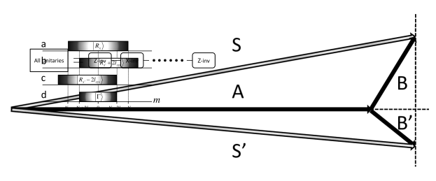
Figure 1: Adding a large vector to a small one: The length of the sums, $S$ and $S^{\prime}$ of the large vector $A$ and the small vectors $B$ and $B^{\prime}$ is almost independent of the components of $B$ and $B^{\prime}$ which is perpendicular to $A$. Lemma II demonstrates the quantum version of this simple property.

Lemma II: Consider the following state

$$\mathopen{|}\psi\mathclose{\rangle}=\mathopen{|}l_{1},m_{1}\mathclose{\rangle}\mathopen{|}l_{2},m_{2}=l_{2}-k\mathclose{\rangle}$$ (5.1)

where $l_{1},l_{2}$ are angular momenta and $m_{1},m_{2}$ are eigenvalues of $L_{Z}$. At the limit of $l_{2}\gg l_{1}^{2},k^{2}$ this state is almost the same as the state with total angular momentum equal to $m_{1}+l_{2}$ and total $L_{z}$ equal to $m_{1}+l_{2}-k$ i.e.

$$\mathopen{|}\phi\mathclose{\rangle}=\mathopen{|}(j=m_{1}+l_{2},m=m_{1}+l_{2}-k):(l_{1},l_{2})\mathclose{\rangle}$$ (5.2)

or more precisely

$$|\mathopen{\langle}\phi\mathclose{|}\psi\rangle|^{2}\geq 1-\frac{(l_{1}^{2}+l_{1}-m_{1}^{2})(2k+1)-m_{1}}{2l_{2}}$$ (5.3)

In terms of Clebsch-Gordon coefficients this means

$$lim_{l_{1}^{2}/l_{2},k^{2}/l_{2}\rightarrow 0}\left(C_{l_{2},l_{2}-k;l_{1},m_{1}}^{m_{1}+l_{2}-k,m_{1}+l_{2}}\right)^{2}=1-\frac{(l_{1}^{2}+l_{1}-m_{1}^{2})(2k+1)-m_{1}}{2l_{2}}$$

This lemma is proven in the appendix. A specific case of these relations is reported in [6] where it is verified numerically.

For $k=0$ we have

$$|\mathopen{\langle}\phi\mathclose{|}\psi\rangle|^{2}\geq 1-\frac{l_{1}^{2}+l_{1}-m_{1}^{2}-m_{1}}{2l_{2}}\geq 1-C^{2}$$ (5.4)

where $C^{2}=\frac{l_{1}^{2}+l_{1}+1/4}{2l_{2}}$ is the minimum of $1-\frac{l_{1}^{2}+l_{1}-m_{1}^{2}-m_{1}}{2l_{2}}$, which occurs for $m_{1}=-1/2$.

Now consider an ancillary system called Z-RF with angular momentum $l_{RZ}$ that is large in comparison with the maximum angular momentum of system $l_{1}$. We assume initially Z-RF is in the state $\mathopen{|}\rm{Z-RF}\mathclose{\rangle}\equiv\mathopen{|}l_{RZ},m_{RZ}=l_{RZ}\mathclose{\rangle}$ and so has maximal angular momentum in the $z$ direction. Following the proof in lemma II, to a very good approximation the total angular momentum of the combined system with Z-RF depends only on $m_{1}$ (the $z$ component of angular momentum of the system)

$$\mathopen{|}l_{1},m_{1},\delta\mathclose{\rangle}\mathopen{|}{\rm Z-RF}\mathclose{\rangle}\approx\mathopen{|}j=m_{1}+l_{RZ},m=m_{1}+l_{RZ},\lambda\mathclose{\rangle}$$ (5.5)

and so is almost independent of $l_{1}$. Here $\delta$ labels possible degeneracies of the state of the physical system and $\lambda$ labels all distinct states of the total system with the same $j=m_{1}+l_{RZ}$ and $m=m_{1}+l_{RZ}$. More precisely $\lambda$ indicates from which $(l_{1},m_{RZ},l_{RZ},\delta)$ the state $\ \mathopen{|}j=m_{1}+l_{RZ},m=m_{1}+l_{RZ},\lambda\mathclose{\rangle}$ is formed. Since $m_{RZ}$ and $l_{RZ}$ are fixed, different $\lambda$’s stand for different $(l_{1},\delta)$’s.

The upshot is that $j$ and $m$ of the combined system are independent of $(l_{1},\delta)$, and depend only on $m_{1}$. Hence we can implement any arbitrary unitary on the subspace of states with the same $m_{1}$ by using an appropriate $U_{\mathscr{R}{\rm-inv}}$. In other words we can implement all unitary time evolutions on the system that commute with $L_{z}$ acting on the system. In the language of quantum information, we implement an arbitrary Z-inv unitary on the system by performing an $R$-inv unitary on the noiseless subsystem of the total system, which consists of the main system and reference frame.

Suppose we are going to implement a unitary time evolution operator $V$ on the system that commutes with $L_{Z}$. $V$ can be written in the form of Eq.(4.5).

Now consider the following decomposition of total Hilbert space of system and Z-RF induced by rotational group

$$\mathscr{H}_{sys}\otimes\mathscr{H}_{Z-RF}\longrightarrow\bigoplus_{j}\ \mathscr{M}_{j}\otimes\mathscr{N}_{j}$$ (5.6)

We define the unitary $\mathscr{V}$ acting on the system and Z-RF to be

$$\mathscr{V}=\bigoplus_{j}I_{j}\otimes V^{(j-l_{RZ})}$$ (5.7)

where $I_{j}$ acts on the gauge subsystem $\mathscr{M}_{j}$, and $V^{(j-l_{RZ})}$ acts on the multiplicity subsystem $\mathscr{N}_{j}$. Obviously $\mathscr{V}$ has the same form as (4.3) and so is isotropic. Note that here we assume this unitary governs the total system (ie. the physical system combined with Z-RF), and so the context of the above formula is for the total system. We assume this unitary acts on the initial state of the total system, which is a tensor product of the initial state of the system and $\mathopen{|}Z-RF\mathclose{\rangle}$.

The effect of this time evolution on the system is described by a superoperator called $\varepsilon^{(1)}$. One possible representation of this time superoperator can be specified by the following set of Kraus operators

$$K_{n}=\mathopen{\langle}l_{RZ},n\mathclose{|}\mathscr{V}\mathopen{|}Z-RF\mathclose{\rangle}=\mathopen{\langle}l_{RZ},n\mathclose{|}\mathscr{V}\mathopen{|}l_{RZ},l_{RZ}\mathclose{\rangle}$$ (5.8)

where $\mathopen{|}l_{RZ},n\mathclose{\rangle}$ is the eigenvector of $L_{Z}$ with eigenvalue $n$. For $K_{l_{RZ}}$ we have

$$K_{l_{RZ}}=\mathopen{\langle}l_{RZ},l_{RZ}\mathclose{|}\mathscr{V}\mathopen{|}l_{RZ},l_{RZ}\mathclose{\rangle}=\sum_{j,\lambda,\lambda^{\prime}}V^{(j-l_{RZ})}_{\lambda,\lambda^{\prime}}\langle l_{RZ},l_{RZ}\mathopen{|}j,j,\lambda\mathclose{\rangle}\mathopen{\langle}j,j,\lambda^{\prime}\mathclose{|}l_{RZ},l_{RZ}\rangle$$

$$+\sum_{j,M<j,\lambda,\lambda^{\prime}}V^{(j-l_{RZ})}_{\lambda,\lambda^{\prime}}\langle l_{RZ},l_{RZ}\mathopen{|}j,M,\lambda\mathclose{\rangle}\mathopen{\langle}j,M,\lambda^{\prime}\mathclose{|}l_{RZ},l_{RZ}\rangle$$ (5.9)

We can rewrite the second term as

$$V^{\prime}\equiv\mathopen{\langle}l_{RZ},l_{RZ}\mathclose{|}(\mathscr{I}-\mathscr{P})\mathscr{V}(\mathscr{I}-\mathscr{P})\mathopen{|}l_{RZ},l_{RZ}\mathclose{\rangle}$$

where $\mathscr{I}$ is the identity operator in the Hilbert space of the combined system and RF, and $\mathscr{P}$ is the projector on the space of all vectors with $M=j$. So the operator $\mathscr{I}-\mathscr{P}$ is the projector to the subspace of states with $M<j.$ For an arbitrary normalized vector $\mathopen{|}\Theta\mathclose{\rangle}$ in the Hilbert space of the physical system we know from Eq.(5.4) that $|(\mathscr{I}-\mathscr{P})\mathopen{|}\Theta\mathclose{\rangle}\mathopen{|}l_{RZ},l_{RZ}\mathclose{\rangle}|\leq C$ where $C^{2}=\frac{l_{1}^{2}+l_{1}+1/4}{2l_{RZ}}$. Since $\mathscr{V}$ is unitary we deduce that $||V^{\prime}||\leq C^{2}$.

To compute the first term in Eq.(5.9) we note that

$$\mathopen{\langle}j,j,\lambda\mathclose{|}(\mathopen{|}l_{1},m,\delta\mathclose{\rangle}\otimes\mathopen{|}l_{RZ},l_{RZ}\mathclose{\rangle})=\delta_{j,m+l_{RZ}}\delta_{\lambda,(l_{1},\delta)}\times\xi_{m,\lambda}$$ (5.10)

where $\xi_{m,\lambda}$ is some real number. From Eq.(5.4) we deduce that $\xi_{m,\lambda}^{2}\geq 1-C^{2}$ and so $\xi_{m,\lambda}^{2}$ is close to one. So using Eq.(5.10) we have

$$\langle l_{RZ},l_{RZ}\mathopen{|}j,j,\lambda\mathclose{\rangle}=\xi_{j-l_{RZ},\lambda}\ \mathopen{|}m=j-l_{RZ},\lambda\mathclose{\rangle}$$ (5.11)

Note that $\lambda$ specifies $l_{1}$ and $\delta$. Now using this equality we see that the first term in Eq.(5.9) can be rewritten as

$$\sum_{j,\lambda,\lambda^{\prime}}V^{(j-l_{Rz})}_{\lambda,\lambda^{\prime}}\langle l_{RZ},l_{RZ}\mathopen{|}j,j,\lambda\mathclose{\rangle}\mathopen{\langle}j,j,\lambda^{\prime}\mathclose{|}l_{RZ},l_{RZ}\rangle=\sum_{m,\lambda,\lambda^{\prime}}V^{(m)}_{\lambda,\lambda^{\prime}}\xi_{m,\lambda}{\xi_{m,\lambda^{\prime}}}\mathopen{|}m,\lambda\mathclose{\rangle}\mathopen{\langle}m,\lambda^{\prime}\mathclose{|}$$ (5.12)

To compute this, first we define

$$X=\langle l_{RZ},l_{RZ}|\mathscr{I}-\mathscr{P}|l_{RZ},l_{RZ}\rangle=I-\sum_{m,\lambda}\xi_{m,\lambda}^{2}\mathopen{|}m,\lambda\mathclose{\rangle}\mathopen{\langle}m,\lambda\mathclose{|}$$ (5.13)

To get the last equality we have used Eq.(5.11). Note that $\xi_{m,\lambda}^{2}\geq 1-C^{2}$ and so $||X||\leq C^{2}$ . Since $\xi_{m,\lambda}$ is close to one we can easily see that $\xi_{m,\lambda}\approx 1/2(1+\xi_{m,\lambda}^{2})$. So we can see Eq.(5.12) equals

$$(I-\frac{X}{2})V(I-\frac{X}{2})\approx V-\frac{1}{2}(VX+XV)$$ (5.14)

So finally $K_{l_{RZ}}=V+\overline{V}$ where $\overline{V}\equiv V^{\prime}-\frac{1}{2}(XV+VX)$. By the triangle inequality we can see that $||\overline{V}||\leq 2C^{2}$. Finally we obtain

$${\varepsilon^{(1)}}(\rho)\approx V\rho V^{\dagger}+\varepsilon^{(1)}_{noise}(\rho)$$ (5.15)

where

$$\varepsilon^{(1)}_{noise}(\rho)=(V\rho{\overline{V}}^{\dagger}+{\overline{V}}\rho V^{\dagger})+\sum_{n<l_{RZ}}K_{n}\rho{K_{n}}^{\dagger}$$ (5.16)

Note that $\varepsilon^{(1)}_{noise}(\rho)$ is not necessarily a positive operator. The first two terms in $\varepsilon^{(1)}_{noise}(\rho)$ commute with $L_{Z}$ and are responsible for the noise in each block of the same $m$. The effect of the last term is that of mixing states with different $m$.

While our target was implementing a unitary time evolution described by $V$, we have instead implemented a time evolution that is described by $\varepsilon^{(1)}$. To estimate the quality of this implementation we compute the distance of these two time evolutions, $d(V(.)V^{\dagger},\varepsilon^{(1)}(.))$:

$$d(V(.)V^{\dagger},\varepsilon^{(1)}(.))=\frac{1}{2}\max_{\rho,\{\mathopen{|}i\mathclose{\rangle}\}}\sum_{i}|\mathopen{\langle}i\mathclose{|}\varepsilon^{(1)}_{noise}(\rho)\mathopen{|}i\mathclose{\rangle}|=\frac{1}{2}\max(\sum_{i}|\mathopen{\langle}i\mathclose{|}(V\rho{\overline{V}}^{\dagger}+{\overline{V}}\rho V^{\dagger})+\sum_{n<l_{RZ}}K_{n}\rho{K_{n}}^{\dagger}\mathopen{|}i\mathclose{\rangle}|)$$ (5.17)

where the maximization is over all bases $\{\mathopen{|}i\mathclose{\rangle}\}$ and all density operators $\rho$. To calculate this quantity first we note that $\sum_{n<l_{RZ}}K_{n}\rho{K_{n}}^{\dagger}$ is a positive operator and so

$$\sum_{i}|\mathopen{\langle}i\mathclose{|}\sum_{n<l_{RZ}}K_{n}\rho{K_{n}}^{\dagger}\mathopen{|}i\mathclose{\rangle}| = tr(\sum_{n<l_{RZ}}K_{n}\rho{K_{n}}^{\dagger})$$ (5.18)

$$= 1-tr(K_{l_{RZ}}\rho{K_{l_{RZ}}}^{\dagger})$$

$$= 1-tr((V+\overline{V})\rho(V+\overline{V})^{\dagger})$$

$$= -tr(V\rho\overline{V}^{\dagger}+\overline{V}\rho V^{\dagger}+\overline{V}\rho\overline{V}^{\dagger})$$

For any set of operators $\{O_{i}\}$ we have $|tr(O_{1}\ldots O_{N}\rho)|\leq||O_{1}||\ldots||O_{N}||$. Using this fact and noting that $||\overline{V}||\leq 2C^{2}$ we can show that for small $C^{2}$ we have

$$tr(\sum_{n<l_{RZ}}K_{n}\rho{K_{n}}^{\dagger})=|tr(V\rho\overline{V}^{\dagger}+\overline{V}\rho V^{\dagger}+\overline{V}\rho\overline{V}^{\dagger})|\leq 4C^{2}$$ (5.19)

On the other hand, we have

$$\sum_{i}|\mathopen{\langle}i\mathclose{|}(V\rho{\overline{V}}^{\dagger}+{\overline{V}}\rho V^{\dagger})\mathopen{|}i\mathclose{\rangle}|\leq\sum_{i}|\mathopen{\langle}i\mathclose{|}V\rho{\overline{V}}^{\dagger}\mathopen{|}i\mathclose{\rangle}|+\sum_{i}|\mathopen{\langle}i\mathclose{|}{\overline{V}}\rho V^{\dagger})\mathopen{|}i\mathclose{\rangle}|$$ (5.20)

Using lemma I we have

$$\sum_{i}|\mathopen{\langle}i\mathclose{|}(V\rho{\overline{V}}^{\dagger}+{\overline{V}}\rho V^{\dagger})\mathopen{|}i\mathclose{\rangle}|\leq 4C^{2}$$ (5.21)

and so

$$d(V(.)V^{\dagger},\varepsilon^{(1)}(.))=\frac{1}{2}\max(\sum_{i}|\mathopen{\langle}i\mathclose{|}\varepsilon^{(1)}_{noise}(\rho)\mathopen{|}i\mathclose{\rangle}|)\leq 4C^{2}$$ (5.22)

Note that to get the same amount of error for different systems, the dimension of RF should increase proportional to the square of the angular momentum of system.

After using the reference frame its state would be changed due to back reaction effects. Since the total $L_{Z}$ is conserved, if there were no error in the implementation of a $Z$-inv unitary, the state of the reference frame would be unchanged. The probability of error is less than $4C^{2}$, so with the probability of $1-4C^{2}$ or more the reference frame stays in its initial state. To get a measure of how the reference frame degrades, consider using it to implement a unitary operation on a different system each time [20]. After using the reference frame $n$ times, as long as $nC^{2}\ll 1$ the probability of being in its initial state would be more than $1-4nC^{2}$ and so the error would be less than $(1-4nC^{2})4C^{2}$. We can see that the state of the reference frame after the first use would be a mixture of states from the set $\{\mathopen{|}l_{RZ},m_{RZ}=l_{RZ}\mathclose{\rangle},\mathopen{|}l_{RZ},m_{RZ}=l_{RZ}-1\mathclose{\rangle},...,\mathopen{|}l_{RZ},m_{RZ}=l_{RZ}-2l_{1}\mathclose{\rangle}\}$.

For a reference frame with fixed $l_{RZ}$, $\mathopen{|}l_{RZ},l_{RZ}\mathclose{\rangle}$ seems to be the best choice. However, taking into account lemma II and the property of adding vectors that we have used in this scheme, we can use other states of the form $\mathopen{|}l_{RZ},m_{RZ}=l_{RZ}-k\mathclose{\rangle}$ provided $l_{RZ}\gg k^{2}$. It is straightforward to see in this case instead of $4C^{2}$ the error would be almost $4C^{2}(2k+1)$.

6 Implementing arbitrary unitaries using $Z$-inv unitaries

In this section we show how to implement all arbitrary unitary time evolutions on a physical system, whether or not they commute with $L_{z}$, by using a $Z$-inv unitary time evolution acting over that physical system combined with an auxiliary reference frame X-RF. We assume the angular momentum of X-RF, $l_{RX}$, is large compared to the maximum angular momentum of the physical system under consideration, $l_{sys}$. The idea is that changes in the angular momentum of the system caused by unitary transformations on the system are compensated for by making changes in X-RF. We choose the initial state of X-RF to have a large uncertainty in $L_{Z}$, such that increasing or decreasing its $L_{Z}$ leaves it nearly unchanged.

We therefore take the initial state of X-RF to be an equal superposition of the form

$$\mathopen{|}R_{X},0\mathclose{\rangle}=\frac{1}{\sqrt{2N+1}}(\mathopen{|}m=-N\mathclose{\rangle}+\ldots+\mathopen{|}m=N\mathclose{\rangle})$$ (6.1)

where $N=l_{RX}-2l_{sys}$, so that the sum is the subset of magnetic quantum numbers within this range. This will afford us freedom to compensate for changes in $L_{z}$ of the system by modifying the state $\mathopen{|}R_{X},0\mathclose{\rangle}$, which we shall denote by $\mathopen{|}R_{X}\mathclose{\rangle}$. Note that the expectation values of $L_{Z}$ and $L_{Y}$ are zero for this state, whereas the expectation value of $L_{X}$ is nonzero, which means that this state is pointing in the X direction. Unlike $\mathopen{|}Z-RF\mathclose{\rangle}$, which is an eigenvector of $L_{Z}$, $\mathopen{|}R_{X}\mathclose{\rangle}$ is not an eigenvector of $L_{X}$ and has completely different character. We shall also deploy the following notation

$$\mathopen{|}R_{X},n\mathclose{\rangle}=\frac{1}{\sqrt{2N+1}}(\mathopen{|}m=-N+n\mathclose{\rangle}+\ldots+\mathopen{|}m=N+n\mathclose{\rangle})$$ (6.2)

which we refer to as a shift of $\mathopen{|}R_{X}\mathclose{\rangle}$ by $n$.

Initially X-RF is in the state $\mathopen{|}R_{X}\mathclose{\rangle}$ which has a large amount of uncertainty in $L_{Z}$. To implement unitaries on the system that do not commute with $L_{Z}$, we compensate for the change in $L_{Z}$ by shifting the state of X-RF such that the total $L_{Z}$ remains constant. Under this change the final state of X-RF is dependent on the state of the system, thereby entangling them. However if $N$ is sufficiently large, which means the initial state has a large uncertainty in $L_{Z}$, these shifts change $\mathopen{|}X-RF\mathclose{\rangle}$ by only a small amount. For very large $N$ the state of system remains unentangled with X-RF.

Our goal is to implement any arbitrary unitary transformation $U$ where

$$U\mathopen{|}m,\lambda\mathclose{\rangle}=\sum_{m^{\prime},\lambda^{\prime}}U_{(m^{\prime},\lambda^{\prime}),(m,\lambda)}\mathopen{|}m^{\prime},\lambda^{\prime}\mathclose{\rangle}$$ (6.3)

and where $\mathopen{|}m,\lambda\mathclose{\rangle}$ is a state of the system. To implement $U$ we construct the following $Z$-inv unitary

$$\mathscr{U}=\bigoplus_{M}\mathscr{U}^{(M)}$$ (6.4)

in which each $\mathscr{U}^{(M)}$ acts in the following manner

$$\mathscr{U}^{(M)}\mathopen{|}m,\lambda\mathclose{\rangle}\mathopen{|}M-m\mathclose{\rangle} = \sum_{m^{\prime},\lambda^{\prime}}U_{(m^{\prime},\lambda^{\prime}),(m,\lambda)}\mathopen{|}m^{\prime},\lambda^{\prime}\mathclose{\rangle}\mathopen{|}M-m^{\prime}\mathclose{\rangle}\quad\ \mathrm{if}\ \ \ |M|\leq N+l_{sys}$$ (6.5)

$$= \mathopen{|}m,\lambda\mathclose{\rangle}\mathopen{|}M-m\mathclose{\rangle}\qquad\qquad\qquad\qquad\qquad\mathrm{if}\ \ |M|>N+l_{sys}$$

where $\mathopen{|}m,\lambda\mathclose{\rangle}$ is in the Hilbert space of the main system and $\mathopen{|}M-m\mathclose{\rangle}$ is in the Hilbert space of X-RF. Using the unitarity of $U$ it is straightforward to check that $\mathscr{U}$ is also a unitary operator that commutes with $L_{Z}$.

Now the effect of $U$ on the initial state $\mathopen{|}m,\lambda\mathclose{\rangle}\mathopen{|}R_{X}\mathclose{\rangle}$ is

$$\mathscr{U}\mathopen{|}m,\lambda\mathclose{\rangle}\mathopen{|}R_{X}\mathclose{\rangle} = \frac{1}{\sqrt{2N+1}}\sum_{M=-N+m}^{N+m}\ \mathscr{U}^{(M)}\mathopen{|}m\mathclose{\rangle}\mathopen{|}M-m\mathclose{\rangle}$$ (6.6)

$$= \frac{1}{\sqrt{2N+1}}\sum_{M=-N+m}^{N+m}\ \ \sum_{m^{\prime},\lambda^{\prime}}U_{(m^{\prime},\lambda^{\prime}),(m,\lambda)}\mathopen{|}m^{\prime},\lambda^{\prime}\mathclose{\rangle}\mathopen{|}M-m^{\prime}\mathclose{\rangle}$$

$$= \frac{1}{\sqrt{2N+1}}\sum_{m^{\prime},\lambda^{\prime}}U_{(m^{\prime},\lambda^{\prime}),(m,\lambda)}\mathopen{|}m^{\prime},\lambda^{\prime}\mathclose{\rangle}\sum_{M=-N+m}^{N+m}\mathopen{|}M-m^{\prime}\mathclose{\rangle}$$

$$= \sum_{m^{\prime},\lambda^{\prime}}U_{(m^{\prime},\lambda^{\prime}),(m,\lambda)}\mathopen{|}m^{\prime},\lambda^{\prime}\mathclose{\rangle}\mathopen{|}R_{X},m-m^{\prime}\mathclose{\rangle}$$

For an arbitrary state of the system $\mathopen{|}\Theta\mathclose{\rangle}=\sum_{m,\lambda}\theta_{m,\lambda}\mathopen{|}m,\lambda\mathclose{\rangle}$ we have

$$\mathscr{U}\mathopen{|}\Theta\mathclose{\rangle}\mathopen{|}R_{X}\mathclose{\rangle}=\sum_{m,\lambda}\theta_{m,\lambda}(\sum_{m^{\prime},\lambda^{\prime}}U_{(m^{\prime},\lambda^{\prime}),(m,\lambda)}\mathopen{|}m^{\prime},\lambda^{\prime}\mathclose{\rangle}\mathopen{|}R_{X},m-m^{\prime}\mathclose{\rangle})$$ (6.7)

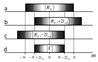
Figure 2: a) The state $\mathopen{|}R_{X}\mathclose{\rangle}$, b) the state $\mathopen{|}R_{X},+2l_{sys}\mathclose{\rangle}$ which is the maximum shifted to the right of $\mathopen{|}R_{X}\mathclose{\rangle}$, c) the state $\mathopen{|}R_{X},-2l_{sys}\mathclose{\rangle}$ which is the maximum shifted to the left of $\mathopen{|}R_{X}\mathclose{\rangle}$ , d) the unnormalized vector $\mathopen{|}\Gamma\mathclose{\rangle}$ which is the common part of all of these states.

So after time evolution the state of system becomes entangled with the state of the reference frame. This entangled state includes a superposition of vectors that are the tensor product of some state of the system and $\mathopen{|}R_{X},m-m^{\prime}\mathclose{\rangle}$, which is the initial state of the reference frame shifted by $m-m^{\prime}$. Since $-l_{sys}\leq m\leq l_{sys}$ the maximum absolute value of these shifts is $2l_{sys}$, yielding the extremal shifted states $\mathopen{|}R_{X},-2l_{sys}\mathclose{\rangle}$ and $\mathopen{|}R_{X},+2l_{sys}\mathclose{\rangle}$. We are interested in the largest common part between all of these shifted states. Therefore we define the unnormalized vector $\mathopen{|}\Gamma\mathclose{\rangle}$ such that the overlap $\mathopen{\langle}\Gamma\mathclose{|}{R_{X},m-m^{\prime}}\rangle$ is maximal and independent of $\{m,m^{\prime}\}$ for all allowed values of $\{m,m^{\prime}\}$ (see fig. 2). We can easily see that

$$\mathopen{|}\Gamma\mathclose{\rangle}=\sqrt{\frac{1}{2N+1}}\sum_{i=-N+2l_{sys}}^{N-2l_{sys}}\mathopen{|}i\mathclose{\rangle}$$ (6.8)

By writing

$$\mathopen{|}R_{X},m-m^{\prime}\mathclose{\rangle}=\mathopen{|}\Gamma\mathclose{\rangle}+\left(\mathopen{|}R_{X},m-m^{\prime}\mathclose{\rangle}-\mathopen{|}\Gamma\mathclose{\rangle}\right)$$ (6.9)

we decompose $\mathopen{|}R_{X},m-m^{\prime}\mathclose{\rangle}$ as superposition of $\mathopen{|}\Gamma\mathclose{\rangle}$ and another vector orthogonal to $\mathopen{|}\Gamma\mathclose{\rangle}$, a result that follows from noting that

$$\langle\Gamma\mathopen{|}R_{X},m-m^{\prime}\mathclose{\rangle}={\langle\Gamma\mathopen{|}\Gamma\mathclose{\rangle}}=\frac{2(N-2l_{sys})+1}{2N+1}$$

Using this decomposition we obtain

$$\mathscr{U}\mathopen{|}\Theta\mathclose{\rangle}\mathopen{|}R_{X}\mathclose{\rangle}=U\mathopen{|}\Theta\mathclose{\rangle}\otimes\mathopen{|}\Gamma\mathclose{\rangle}+\sum_{m,\lambda}\theta_{m,\lambda}\sum_{m^{\prime},\lambda^{\prime}}U_{(m^{\prime},\lambda^{\prime}),(m,\lambda)}\mathopen{|}m^{\prime},\lambda^{\prime}\mathclose{\rangle}(\mathopen{|}R_{X},m-m^{\prime}\mathclose{\rangle}-\mathopen{|}\Gamma\mathclose{\rangle})$$ (6.10)

This describes the total state of the system and X-RF after this time evolution. To find the effect of this time evolution on the system we trace over the Hilbert space of X-RF. This yields a superoperator that maps the initial state of system, $\rho$ to

$$\varepsilon^{(2)}(\rho)=\mathopen{\langle}\Gamma\mathclose{|}\Gamma\rangle U\rho U^{\dagger}+(1-\mathopen{\langle}\Gamma\mathclose{|}\Gamma\rangle)\varepsilon_{noise}^{(2)}(\rho)=\frac{2(N-2l_{sys})+1}{2N+1}U\rho U^{\dagger}+\frac{4l_{sys}}{2N+1}\varepsilon_{noise}^{(2)}(\rho)$$ (6.11)

where $\varepsilon_{noise}^{(2)}$ is a trace-preserving completely positive super-operator. So using Eq.(3.4) we see that the error in the outcome probability of any arbitrary measurement is less than $d(U(.)U^{\dagger},\varepsilon^{(2)})\leq\frac{4l_{sys}}{2N+1}$. In the limit of large $N/l_{sys}$ the error rate, $2l_{sys}/N$, is small.

7 The First Scheme

In section 5 we saw how an $R$-inv time evolution acting on the physical system and Z-RF can be used to implement any arbitrary $Z$-inv unitary on the physical system. Then in section 6 we saw how a $Z$-inv unitary time evolution acting on the main system and X-RF can be used to implement any arbitrary unitary on the physical system. By combining these two schemes we can perform any arbitrary unitary on the system just by using $R$-inv unitary time evolutions and Z-RF and X-RF (see fig. 3).

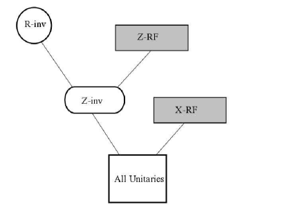
Figure 3: Schematic description of scheme 1.

To implement an arbitrary unitary $U$ acting on the system, we need to implement the $Z$-inv unitary $\mathscr{U}$ (defined in the previous section) on the system coupled to the auxiliary X-RF. To do so we let the $R$-inv unitary $\mathscr{V}=\sum_{j}I_{j}\otimes\mathscr{U}^{(j-l_{RZ})}$ act on the system coupled to both X-RF and Z-RF. Initially the density matrix is

$$\rho^{sys}\otimes\mathopen{|}R_{X}\mathclose{\rangle}\mathopen{\langle}R_{X}\mathclose{|}\otimes\mathopen{|}Z-RF\mathclose{\rangle}\mathopen{\langle}Z-RF\mathclose{|}$$ (7.1)

After the time evolution the state of the system is

$$\varepsilon(\rho)=tr_{Z-RF,X-RF}(\mathscr{V}\rho^{sys}\otimes\mathopen{|}R_{X}\mathclose{\rangle}\mathopen{\langle}R_{X}\mathclose{|}\otimes\mathopen{|}Z-RF\mathclose{\rangle}\mathopen{\langle}Z-RF\mathclose{|}\mathscr{V}^{\dagger})$$ (7.2)

$\mathscr{V}$ is designed to implement $\mathscr{U}$ on the physical system and X-RF. So

$$\varepsilon(\rho)=tr_{X-RF}(\mathscr{U}\rho^{sys}\otimes\mathopen{|}R_{X}\mathclose{\rangle}\mathopen{\langle}R_{X}\mathclose{|}\mathscr{U}^{\dagger})+tr_{X-RF}(\varepsilon^{(1)}_{noise}(\rho^{sys}\otimes\mathopen{|}R_{X}\mathclose{\rangle}\mathopen{\langle}R_{X}\mathclose{|}))$$ (7.3)

From Eq.(6.11) we know that for large $N$

$$\varepsilon(\rho)=\frac{N-2l_{sys}}{N}U\rho U^{\dagger}+\frac{2l_{sys}}{N}\varepsilon_{noise}^{(2)}(\rho)+tr_{X-RF}(\varepsilon^{(1)}_{noise}(\rho^{sys}\otimes\mathopen{|}R_{X}\mathclose{\rangle}\mathopen{\langle}R_{X}\mathclose{|}))$$

$$=\frac{N-2l_{sys}}{N}U\rho U^{\dagger}+\varepsilon_{noise}(\rho)$$ (7.4)

where

$$\varepsilon_{noise}(\rho)=\frac{2l_{sys}}{N}\varepsilon_{noise}^{(2)}(\rho)+tr_{X-RF}(\varepsilon^{(1)}_{noise}(\rho^{sys}\otimes\mathopen{|}R_{X}\mathclose{\rangle}\mathopen{\langle}R_{X}\mathclose{|}))$$ (7.5)

To estimate the accuracy of this implementation we find an upper bound for $d(U(.)U^{\dagger},\varepsilon(.))$

$$d(U(.)U^{\dagger},\varepsilon(.)) = \frac{1}{2}\max_{\rho,\{\mathopen{|}i\mathclose{\rangle}\}}\sum_{i}|\mathopen{\langle}i\mathclose{|}U\rho U^{\dagger}-\varepsilon(\rho)\mathopen{|}i\mathclose{\rangle}|$$ (7.6)

$$= \frac{1}{2}\max_{\rho,\{\mathopen{|}i\mathclose{\rangle}\}}\sum_{i}\left|\mathopen{\langle}i\mathclose{|}\frac{2l_{sys}}{N}U\rho U^{\dagger}-\frac{2l_{sys}}{N}\varepsilon_{noise}^{(2)}(\rho)\right.$$

$$\qquad-\left.tr_{X-RF}(\varepsilon^{(1)}_{noise}(\rho^{sys}\otimes\mathopen{|}R_{X}\mathclose{\rangle}\mathopen{\langle}R_{X}\mathclose{|}))\mathopen{|}i\mathclose{\rangle}\right|$$

Using the triangle inequality and noting that $\varepsilon_{noise}^{(2)}$ is positive and trace-preserving, we find

$$d(U(.)U^{\dagger},\varepsilon(.)) \leq \frac{2l_{sys}}{N}+\frac{1}{2}\max_{\rho,\{\mathopen{|}i\mathclose{\rangle}\}}\sum_{i}|\mathopen{\langle}i\mathclose{|}tr_{X-RF}(\varepsilon^{(1)}_{noise}(\rho^{sys}\otimes\mathopen{|}R_{X}\mathclose{\rangle}\mathopen{\langle}R_{X}\mathclose{|}))\mathopen{|}i\mathclose{\rangle}|$$ (7.7)

$$< \frac{2l_{sys}}{N}+\frac{1}{2}\max_{\rho,\{\mathopen{|}i\mathclose{\rangle}\}}\sum_{i,s}|\mathopen{\langle}i\mathclose{|}\mathopen{\langle}s\mathclose{|}\varepsilon^{(1)}_{noise}(\rho^{sys}\otimes\mathopen{|}R_{X}\mathclose{\rangle}\mathopen{\langle}R_{X}\mathclose{|})\mathopen{|}s\mathclose{\rangle}\mathopen{|}i\mathclose{\rangle}|$$

where $\{\mathopen{|}s\mathclose{\rangle}\}$ is orthogonal basis in the Hilbert space of X-RF. Using Eq.(5.22) we can find an upper bound for the last term in the right-hand side of the above equation. Since the angular momentum of X-RF is $N+2l_{sys}$, the maximum total angular momentum of the system and X-RF is $l_{1}=N+3l_{sys}$. However since $N\gg l_{sys}$ we can assume $l_{1}\approx N$. Thus using Eq.(5.22) and noting that $C^{2}=\frac{l_{1}^{2}+l_{1}+1/4}{2l_{RZ}}$ we obtain

$$d(U(.)U^{\dagger},\varepsilon(.))\leq\frac{2l_{sys}}{N}+\frac{2N^{2}}{l_{RZ}}$$ (7.8)

where $l_{RZ}\gg N$. Obviously by choosing larger $l_{RZ}$ the error becomes smaller. For any given $l_{RZ}$ there is a specific $N$ that minimizes this error. After minimizing with respect to $N$ we have

$$error_{I}(l_{sys},l_{RF})=3\left(\frac{2l_{sys}^{2}}{l_{RZ}}\right)^{1/3}$$ (7.9)

where $error_{I}$ shows the error in scheme I as a function of the maximum angular momentum $l_{sys}$ of the system and the angular momentum $l_{RF}$ of reference frame. We shall discuss the implications of this result in section 9.

8 The Second Scheme

In this section we propose an alternative method for building an arbitrary unitary time evolution by using $R$-inv time evolutions. As we have seen in section 5 we can implement all $Z$-inv unitary evolutions by using $R$-inv unitary time evolutions and a reference frame in the z direction. In the same way we can build all unitaries commuting with $L_{X}$ ($X$-inv unitaries) by using a reference frame X-RF that is defined in the same way as Z-RF, but rotated so that the x direction is now the specified direction. Note that the X-RF we use in this scheme differs from the one we used in the first scheme. Now by a sequence of $Z$-inv and $X$-inv unitaries we can build more unitary time evolutions. In fact, as we will show in the following, from a sequence of unitaries alternately commuting with $L_{X}$ and $L_{Z}$ we can build any arbitrary unitary (see fig. 4).

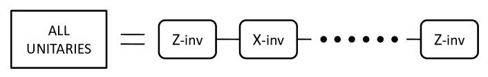
Figure 4: Schematic description of scheme 2: building all unitaries using a sequence of $Z-inv$ and $X-inv$ unitaries.

The main idea is based on the following property using the four Hamiltonians $\pm H_{1}$ and $\pm H_{2}$. By sequentially applying these Hamiltonians we can construct any arbitrary Hamiltonian contained in the Lie algebra generated by $\{H_{1},H_{2}\}$. Consider the following example. Apply $H_{1}$, followed by $H_{2}$,$-H_{1}$, and $-H_{2}$, each for the same time $\delta t$. Since

$$e^{iH_{1}\delta t}e^{iH_{2}\delta t}e^{-iH_{1}\delta t}e^{-iH_{2}\delta t}=e^{i(H_{1}H_{2}-H_{2}H_{1})\delta t^{2}}+O(\delta t^{3})$$ (8.1)

for small $\delta t$, the result is the same as if one had applied $i[H_{1},H_{2}]$ for time $\delta t^{2}$. In general, any given Hamiltonian in the Lie algebra generated by $H_{1}$ and $H_{2}$, can effectively be constructed by applying a sequence of $\pm H_{1}$ and $\pm H_{2}$ [21].

Using $R$-inv interactions acting on the system and reference frames, we are able to apply all Hamiltonians commuting with $L_{Z}$ and also all Hamiltonians commuting with $L_{X}$ by using Z-RF and X-RF respectively . The Lie algebra generated by these generators describes the full set of Hamiltonians that can be constructed. The following lemma illustrates how to find this Lie algebra.

Lemma III Suppose $A$,$B$ are two Hermitian operators with the property that no eigensubspace of $A$ is orthogonal to any eigensubspace of $B$. Then the union of the set of all unitaries commuting with $A$ and the set of all unitaries commuting with $B$ is a universal set i.e. all unitary operators can be constructed from a sequence of unitaries in those sets. Moreover the length of required sequence is uniformly bounded.

This lemma is proven in the appendix. (It has a nice generalization based on graph connectivity to an arbitrary number of operators (instead of just $A$ and $B$) [22].) In any representation $L_{Z}$ and $L_{X}$ have the property that no eigensubspace of $L_{X}$ is orthogonal to an eigensubspace of $L_{Z}$. Consequently unitary operators commuting with $L_{Z}$ and unitary operators commuting with $L_{X}$ form a universal set.

Each time we use a reference frame it experiences some inevitable backreaction [8, 7]. For instance after performing a Z-inv time evolution on the system, the Z-RF is not in its initial state $\mathopen{|}Z-RF\mathclose{\rangle}=\mathopen{|}l_{RZ},l_{RZ}\mathclose{\rangle}$ anymore, but instead is in a mixture of states including states with other magnetic quantum numbers. This new state of Z-RF cannot specify the z direction as well as the initial state. So it cannot be corrected to get the initial state of Z-RF by just using R-inv resources without using another Z-RF. We might employ this used Z-RF to perform the next Z-inv time evolution; however since this used Z-RF cannot specify z direction as well as the initial Z-RF we expect more noise in implementing the second Z-inv time evolution. Consequently to avoid increasing amounts of noise we need a fresh reference frame after each use (or after several uses) when the Z-RF is degraded more than some specific threshold, dependent on the desired accuracy. Considering the reference frames as a resource it is important to know the number needed to implement a unitary time evolution with some precision. The length of the required sequence is uniformly bounded, which means that there exists an upper bound for the number of steps required to build any arbitrary unitary. How can we estimate this number? In other words, how many times do we need to use those reference frames?

To answer this question we employ the Solovay-Kitaev theorem. According to this theorem if $G$ is a universal set of unitary operators which produce a dense subset of $SU(d)$, and $G$ is closed under inverse then $\forall U\in SU(d),\tau>0,\exists U_{1},...,U_{n}\in G$ such that $||U-U_{1}...U_{n}||\leq\tau$ and $n=\mathscr{O}(\ln^{2}(\frac{1}{\tau}))$ [16].

In the present case $G$ consists of unitaries commuting with $L_{Z}$ and unitaries commuting with $L_{X}$. Suppose $U_{apx}$ is the approximation of $U$ that is obtained by this method after $n$ steps $U_{apx}=U_{1}...U_{n}$ where $||U-U_{apx}||\leq\tau$. According to the Solovay-Kitaev theorem we can assume $n\approx A\ln^{2}(\frac{1}{\tau})$ where $A$ is a constant. Using Eq.(3.8) and assuming $\tau$ is small we find $d(U(.)U^{\dagger},U_{apx}(.)U_{apx}^{\dagger})\leq\tau$.

Due to the finite size of the reference frame we cannot perform $U_{1},...,U_{n}$ perfectly; each time there is an error less than $4C^{2}$. So instead of $U_{1}...U_{n}(.)U^{\dagger}_{n}...U_{1}^{\dagger}$ we implement $\varepsilon(.)=\varepsilon_{1}(...\varepsilon_{n}(.))$. Using the triangle inequality we have

$$d(U(.)U^{\dagger},\varepsilon(.))\leq d(U(.)U^{\dagger},U_{apx}(.)U_{apx}^{\dagger})+d(U_{apx}(.)U_{apx}^{\dagger},\varepsilon(.))\leq\tau+4nC^{2}=\tau+4A\ C^{2}\ln^{2}(\frac{1}{\tau})$$ (8.2)

where Eq. (3.2) was repeatedly used to bound $d(U_{apx}(.)U_{apx}^{\dagger},\varepsilon(.))$.

The angular momentum of the reference frame, which is proportional to $1/C^{2}$, and the required number of reference frames $n$ both can be regarded as limiting resources. In terms of these resources total error is bounded by

$$e^{-\sqrt{n/A}}+4nC^{2}$$

Obviously increasing the angular momentum of the reference frame decreases $C^{2}$ and with it the error. As $C^{2}\to 0$ this error approaches zero. However given a fixed $C^{2}$, what is the minimum total error we can achieve under this restriction? By minimizing the total error $\tau+4A\ C^{2}\ln^{2}(\frac{1}{\tau})$ with respect to $\tau$ we can find the minimum accessible error under this constraint. Defining $\tau=e^{-\sigma}$ and $x=(8AC^{2})^{-1}$ the minimizing condition is

$$x=\sigma e^{\sigma}\Longrightarrow\sigma=W(x)$$ (8.3)

where $W(x)$ is the Lambert-W function [23].

Figure 5: Error in scheme II as a function of $x$ where $x\propto l_{RF}/l^{2}_{sys}$

Hence the total error is bounded by

$$e^{-W(x)}+x^{-1}W^{2}(x)$$

(see fig.5) and the number of reference frames we need would be $AW^{2}(x)$. Note that $x$ is equal to some constant times $l_{RF}/l^{2}_{sys}$. For $x>1$ we can see that $\ln(x)/2<W(x)<\ln(x)$. So at the limit of large $x$ the error is bounded by

$$error_{II}(l_{sys},l_{RF})=\ln^{2}(x)/x$$ (8.4)

and the number of required reference frames grows like $\ln^{2}(x)$.

Finally we note that, though non-optimal, we can of course choose any other direction instead of the x direction (except Z) for the second reference frame. However a bad choice of independent direction necessitates a longer sequence to reach an arbitrary unitary.

9 Discussion

Associated with any restriction on resources is a theory describing whether under certain constraints a given operation is feasible. Entanglement resource theory is a well-known example. Analogously, a resource theory has more recently been developed for reference frames [18]. It is interesting to compare the two schemes proposed here from the viewpoint of the resources they require.

First note that the error in both of these schemes is a function of $l_{sys}^{2}/l_{RF}$. Hence if the maximum angular momentum of the system increases by a factor of $k$ then an increase in the angular momentum of the reference frame by a factor of $k^{2}$ will yield the same error. It is not clear whether there exist schemes in which this factor is smaller than $k^{2}$.

Now let us check how the error decreases as the (large) reference-frame angular momentum increases in these two schemes. Looking to eqs. (7.9,8.4) we see that in the first scheme the reciprocal of the error grows as $\mathscr{O}(\sqrt[3]{l_{RF}})$ while in the second scheme it grows as $\mathscr{O}(l_{RF}/\ln^{2}(l_{RF}))$ . Recall that both these schemes are based on a simpler scheme to implement $Z-inv$ unitary time evolutions in which the reciprocal error is $\mathscr{O}(l_{RF})$. So it seems reasonable that the reciprocal of the error in both of these schemes grows slower than $\mathscr{O}(l_{RF})$. A natural open problem is to determine the best scheme for ensuring the error tends to zero as rapidly as possible relative to $l_{RF}$.

We have shown that the presence of rotational symmetry does not restrict us in performing arbitrary measurements or time evolutions of the system. As there is evidently nothing specific in rotational symmetry, we expect that the same holds for the existence of other symmetries. For example an extension of these results to more complicated Lie groups, such as $SU(N)$, would be interesting. Here the challenge is to construct an appropriate generalization of lemma II. Apart from this, there is nothing specific to SU(2) that would appear to prohibit this kind of generalization. Work on this issue is in progress.

Acknowledgments

We are grateful to Lana Sheridan, Easwar Magesan and David Poulin for reading the manuscript and providing important comments and introducing some references. We thank Robert Spekkens for valuable discussions. This work was supported by the Natural Sciences and Engineering Research Council of Canada.

Appendix: Proofs of the Lemmas

Lemma I:

Suppose $\rho$ is a density operator and $O_{1},O_{2}$ are two arbitrary operators and $\{\mathopen{|}i\mathclose{\rangle}\}$ is an arbitrary set of an orthogonal basis. Then

$$\sum_{i}|\mathopen{\langle}i\mathclose{|}O_{1}\rho O_{2}\mathopen{|}i\mathclose{\rangle}|\leq||O_{1}||\times||O_{2}||$$

Proof

Using the Cauchy-Schwartz inequality we have

$$\sum_{i}|\mathopen{\langle}i\mathclose{|}O_{1}\rho O_{2}\mathopen{|}i\mathclose{\rangle}|=\sum_{i}|\mathopen{\langle}i\mathclose{|}O_{1}\sqrt{\rho}\sqrt{\rho}O_{2}\mathopen{|}i\mathclose{\rangle}|\leq\sqrt{\sum_{i}{\mathopen{\langle}i\mathclose{|}O_{1}\rho O_{1}^{\dagger}\mathopen{|}i\mathclose{\rangle}}}\sqrt{\sum_{i}{\mathopen{\langle}i\mathclose{|}O_{2}\rho O_{2}^{\dagger}\mathopen{|}i\mathclose{\rangle}}}$$ (9.1)

$$=\sqrt{tr(|O_{1}|^{2}\rho)tr(|O_{2}|^{2}\rho)}\leq||O_{1}||\times||O_{2}||$$ (9.2)

Using this result we can get the more general result that

$$\sum_{i}|\mathopen{\langle}i\mathclose{|}O_{1}\ldots O_{k}\rho O_{k+1}\ldots O_{N}\mathopen{|}i\mathclose{\rangle}|\leq||O_{1}||\ldots||O_{N}||$$ (9.3)

Lemma II

Consider the following state

$$\mathopen{|}\psi\mathclose{\rangle}=\mathopen{|}l_{1},m_{1}\mathclose{\rangle}\mathopen{|}l_{2},m_{2}=l_{2}-k\mathclose{\rangle}$$ (9.4)

where $l_{1},l_{2}$ are angular momentums and $m_{1},m_{2}$ are eigenvalues of $L_{Z}$. At the limit of $l_{2}\gg l_{1}^{2},k^{2}$ this state is almost the same as the state with total angular momentum equal to $m_{1}+l_{2}$ and total $L_{z}$ equal to $m_{1}+l_{2}-k$ i.e.

$$\mathopen{|}\phi\mathclose{\rangle}=\mathopen{|}(j=m_{1}+l_{2},m=m_{1}+l_{2}-k):(l_{1},l_{2})\mathclose{\rangle}$$ (9.5)

or more precisely

$$|\mathopen{\langle}\phi\mathclose{|}\psi\rangle|^{2}\geq 1-\frac{(l_{1}^{2}+l_{1}-m_{1}^{2})(2k+1)-m_{1}}{2l_{2}}$$ (9.6)

In terms of Clebsch-Gordon coefficients this means

$$lim_{l_{1}^{2}/l_{2},k^{2}/l_{2}\rightarrow 0}\left(C_{l_{2},l_{2}-k;l_{1},m_{1}}^{m_{1}+l_{2}-k,m_{1}+l_{2}}\right)^{2}=1-\frac{(l_{1}^{2}+l_{1}-m_{1}^{2})(2k+1)-m_{1}}{2l_{2}}$$

Proof

Define $m_{tot}=m_{1}+l_{2}-k$. For $i\geq m_{tot}$ we denote

$$\mathopen{|}i\mathclose{\rangle}\equiv\mathopen{|}(j=i,m=m_{tot}):(l_{1},l_{2})\mathclose{\rangle}$$ (9.7)

Using this notation we can expand $\mathopen{|}\psi\mathclose{\rangle}$ as

$$\mathopen{|}\psi\mathclose{\rangle}=\alpha\mathopen{|}\phi\mathclose{\rangle}+\sum_{i=m_{tot},i\neq l_{tot}}^{l_{1}+l_{2}}\beta_{i}\mathopen{|}i\mathclose{\rangle}$$ (9.8)

where $l_{tot}=m_{1}+l_{2}$ and $\mathopen{|}\phi\mathclose{\rangle}$, which is defined in the lemma is actually the state $\mathopen{|}(j=l_{tot},m=m_{tot}):(l_{1},l_{2})\mathclose{\rangle}$. Note that $L_{z}\mathopen{|}\psi\mathclose{\rangle}=m_{tot}\mathopen{|}\psi\mathclose{\rangle}$ and so vector states with total angular momentum less than $m_{tot}$ do not appear in this expansion. Using this expansion we have

$$J^{2}\mathopen{|}\psi\mathclose{\rangle}=\alpha l_{tot}(l_{tot}+1)\mathopen{|}\phi\mathclose{\rangle}+\sum_{i=m_{tot},i\neq l_{tot}}^{l_{1}+l_{2}}i(i+1)\beta_{i}\mathopen{|}i\mathclose{\rangle}$$ (9.9)

$$=\alpha l_{tot}(l_{tot}+1)\mathopen{|}\phi\mathclose{\rangle}+\sum_{i=m_{tot},i\neq l_{tot}}^{l_{1}+l_{2}}l_{tot}(l_{tot}+1)\beta_{i}\mathopen{|}i\mathclose{\rangle}+\sum_{i=m_{tot},i\neq l_{tot}}^{l_{1}+l_{2}}[i(i+1)-l_{tot}(l_{tot}+1)]\beta_{i}\mathopen{|}i\mathclose{\rangle}$$ (9.10)

$$=l_{tot}(l_{tot}+1)\mathopen{|}\psi\mathclose{\rangle}+\sum_{i=m_{tot},i\neq l_{tot}}^{l_{1}+l_{2}}[i(i+1)-l_{tot}(l_{tot}+1)]\beta_{i}\mathopen{|}i\mathclose{\rangle}$$ (9.11)

On the other hand, using the relation

$$J^{2}=L_{1}^{2}+L_{2}^{2}+2\overrightarrow{L}_{1}.\overrightarrow{L}_{2}=L_{1}^{2}+L_{2}^{2}+2L_{1z}L_{2z}+L_{1+}L_{2-}+L_{1-}L_{2+}$$ (9.12)

we obtain

$$J^{2}\mathopen{|}\psi\mathclose{\rangle}=[l_{1}(l_{1}+1)+l_{2}(l_{2}+1)+2m_{1}(l_{2}-k)]\mathopen{|}\psi\mathclose{\rangle}+$$

$$\sqrt{(l_{1}+m_{1}+1)(l_{1}-m_{1})}\sqrt{(2l_{2}-k)(1+k)}\mathopen{|}\psi_{1}^{\bot}\mathclose{\rangle}+\sqrt{(l_{1}-m_{1}+1)(l_{1}+m_{1})}\sqrt{k(2l_{2}-k+1)}\mathopen{|}\psi_{2}^{\bot}\mathclose{\rangle}$$ (9.13)

Where

$$\mathopen{|}\psi_{1}^{\bot}\mathclose{\rangle}=\mathopen{|}l_{1},m_{1}+1\mathclose{\rangle}\otimes\mathopen{|}l_{2},m_{2}=l_{2}-k-1\mathclose{\rangle}\ ,\ \ \mathopen{|}\psi_{2}^{\bot}\mathclose{\rangle}=\mathopen{|}l_{1},m_{1}-1\mathclose{\rangle}\otimes\mathopen{|}l_{2},m_{2}=l_{2}-k+1\mathclose{\rangle}$$

are orthogonal to $\mathopen{|}\psi\mathclose{\rangle}$.
Equating this result with Eq.(9.11) we obtain

$$\sum_{i=m_{tot},i\neq l_{tot}}^{l_{1}+l_{2}}[i(i+1)-l_{tot}(l_{tot}+1)]\beta_{i}\mathopen{|}i\mathclose{\rangle}=A\mathopen{|}\psi\mathclose{\rangle}+B\mathopen{|}\psi_{1}^{\bot}\mathclose{\rangle}+D\mathopen{|}\psi_{2}^{\bot}\mathclose{\rangle}$$ (9.14)

where

$$A=l_{1}(l_{1}+1)-m_{1}(m_{1}+1)-2m_{1}k\,\ \ \ B=\sqrt{(l_{1}+m_{1}+1)(l_{1}-m_{1})(2l_{2}-k)(1+k)}\$$

$$D=\sqrt{(l_{1}-m_{1}+1)(l_{1}+m_{1})k(2l_{2}-k+1)}$$ (9.15)

So we deduce that

$$\sum_{i=m_{tot},i\neq l_{tot}}^{l_{1}+l_{2}}[i(i+1)-l_{tot}(l_{tot}+1)]^{2}|\beta_{i}|^{2}=A^{2}+B^{2}+D^{2}$$ (9.16)

Now we find the lower bound for the left-hand side of Eq.(9.16) for a fixed value of $\sum|\beta_{i}|^{2}=1-\alpha^{2}$. The minimum of this expression occurs when all $\beta_{i}$ are zero except that one for which the factor $[i(i+1)-l_{tot}(l_{tot}+1)]^{2}$ is minimum. For $k>0$ this minimum occurs when $i=l_{tot}-1$. For $k=0$, $i$ is larger than $l_{tot}$ and so this minimum happens for $i=l_{tot}+1$. Putting these $\beta_{i}$s in Eq.(9.16) and noting that $|\alpha|^{2}=1-\sum|\beta_{i}|^{2}$ we obtain

$$A^{2}+B^{2}+D^{2}=\sum_{i=m_{tot},i\neq l_{tot}}^{l_{1}+l_{2}}[i(i+1)-l_{tot}(l_{tot}+1)]^{2}|\beta_{i}|^{2}\geq(1-|\alpha|^{2})|2l_{tot}|^{2}$$ (9.17)

or equivalently

$$|\alpha|^{2}\geq 1-\frac{(A^{2}+B^{2}+D^{2})}{4|l_{tot}|^{2}}$$ (9.18)

This inequality is always true for all $l_{1},l_{2},k$. Now we assume $l_{2}\gg l_{1}^{2},k^{2}$ and so we obtain

$$|\alpha|^{2}\geq 1-\frac{(l_{1}^{2}+l_{1}-m_{1}^{2})(2k+1)-m_{1}}{2l_{2}}$$ (9.19)

Lemma III

Suppose $A$,$B$ are two Hermitian operators with the property that no eigensubspace of $A$ is orthogonal to any eigensubspace of $B$. Then the union of the set of all unitaries commuting with $A$ and the set of all unitaries commuting with $B$ is a universal set i.e. all unitary operators can be constructed from a sequence of unitaries in those sets. Moreover the length of the required sequence is uniformly bounded.

Proof

We define $\mathscr{H}$ to be the linear space spanned by all Hamiltonians that can be constructed by a sequence of applying Hamiltonians commuting with $A$ and Hamiltonians commuting with $B$. Suppose $\{\mathopen{|}\alpha_{i},\sigma_{i}\mathclose{\rangle}\}$ are the eigenvectors of $A$ with eigenvalue $\alpha_{i}$ and $\{\mathopen{|}\beta_{j},\zeta_{j}\mathclose{\rangle}\}$ are eigenvectors of $B$ with eigenvalue $\beta_{j}$ where $\sigma_{i}$ and $\zeta_{j}$ shows possible degeneracies. From the assumption of this lemma we know that all of the following operators are in $\mathscr{H}$.

$$\{\mathopen{|}\alpha_{i},\sigma_{i}\mathclose{\rangle}\mathopen{\langle}\alpha_{i},\sigma^{\prime}_{i}\mathclose{|}\}\bigcup\{\mathopen{|}\beta_{j},\zeta_{j}\mathclose{\rangle}\mathopen{\langle}\beta_{j},\zeta^{\prime}_{j}\mathclose{|}\}$$

Moreover we know that $\mathscr{H}$ is closed under commutation. So the following operators is also in $\mathscr{H}$

$$[\mathopen{|}\alpha_{i},\sigma_{i}\mathclose{\rangle}\mathopen{\langle}\alpha_{i},\sigma_{i}\mathclose{|},\mathopen{|}\beta_{j},\zeta_{j}\mathclose{\rangle}\mathopen{\langle}\beta_{j},\zeta_{j}\mathclose{|}]=\mathopen{\langle}\alpha_{i},\sigma_{i}\mathclose{|}\beta_{j},\zeta_{j}\rangle\mathopen{|}\alpha_{i},\sigma_{i}\mathclose{\rangle}\mathopen{\langle}\beta_{j},\zeta_{j}\mathclose{|}-\mathopen{\langle}\beta_{j},\zeta_{j}\mathclose{|}\alpha_{i},\sigma_{i}\rangle\mathopen{|}\beta_{j},\zeta_{j}\mathclose{\rangle}\mathopen{\langle}\alpha_{i},\sigma_{i}\mathclose{|}$$ (9.20)

From the assumptions of the lemma, we also know that for each pair of $\alpha_{i},\beta_{j}$ there exist some $\sigma_{i},\zeta_{j}$ such that $\mathopen{\langle}\alpha_{i},\sigma_{i}\mathclose{|}\beta_{j},\zeta_{j}\rangle\neq 0$ and so the following operator is a member of $\mathscr{H}$.

$$e^{i\theta}\mathopen{|}\alpha_{i},\sigma_{i}\mathclose{\rangle}\mathopen{\langle}\beta_{j},\zeta_{j}\mathclose{|}-e^{-i\theta}\mathopen{|}\beta_{j},\zeta_{j}\mathclose{\rangle}\mathopen{\langle}\alpha_{i},\sigma_{i}\mathclose{|}$$ (9.21)

where $e^{i\theta}\equiv\mathopen{\langle}\alpha_{i},\sigma_{i}\mathclose{|}\beta_{j},\zeta_{j}\rangle/|\mathopen{\langle}\alpha_{i},\sigma_{i}\mathclose{|}\beta_{j},\zeta_{j}\rangle|$. Also the commutator of this operator with $\mathopen{|}\beta_{j},\zeta_{j}\mathclose{\rangle}\mathopen{\langle}\beta_{j},\zeta^{\prime}_{j}\mathclose{|}+\mathopen{|}\beta_{j},\zeta^{\prime}_{j}\mathclose{\rangle}\mathopen{\langle}\beta_{j},\zeta_{j}\mathclose{|}$ is a member of $\mathscr{H}$

$$[\ e^{i\theta}\mathopen{|}\alpha_{i},\sigma_{i}\mathclose{\rangle}\mathopen{\langle}\beta_{j},\zeta_{j}\mathclose{|}-e^{-i\theta}\mathopen{|}\beta_{j},\zeta_{j}\mathclose{\rangle}\mathopen{\langle}\alpha_{i},\sigma_{i}\mathclose{|}\ ,\ \mathopen{|}\beta_{j},\zeta_{j}\mathclose{\rangle}\mathopen{\langle}\beta_{j},\zeta^{\prime}_{j}\mathclose{|}+\mathopen{|}\beta_{j},\zeta^{\prime}_{j}\mathclose{\rangle}\mathopen{\langle}\beta_{j},\zeta_{j}\mathclose{|}\ ]$$

$$=e^{i\theta}\mathopen{|}\alpha_{i},\sigma_{i}\mathclose{\rangle}\mathopen{\langle}\beta_{j},\zeta^{\prime}_{j}\mathclose{|}+e^{-i\theta}\mathopen{|}\beta_{j},\zeta^{\prime}_{j}\mathclose{\rangle}\mathopen{\langle}\alpha_{i},\sigma_{i}\mathclose{|}+c_{1}\mathopen{|}\beta_{j},\zeta_{j}\mathclose{\rangle}\mathopen{\langle}\beta_{j},\zeta^{\prime}_{j}\mathclose{|}+c_{1}^{*}\mathopen{|}\beta_{j},\zeta^{\prime}_{j}\mathclose{\rangle}\mathopen{\langle}\beta_{j},\zeta_{j}\mathclose{|}+c_{2}\mathopen{|}\beta_{j},\zeta_{j}\mathclose{\rangle}\mathopen{\langle}\beta_{j},\zeta_{j}\mathclose{|}$$

where $c_{1}$ is a complex number and $c_{2}$ is real and moreover we have assumed $\zeta_{j}\neq\zeta^{\prime}_{j}$. But the terms with coefficients $c_{1}$ and $c_{2}$ are members of $\mathscr{H}$ and $\mathscr{H}$ is closed under linear combination. So we deduce that $e^{i\theta}\mathopen{|}\alpha_{i},\sigma_{i}\mathclose{\rangle}\mathopen{\langle}\beta_{j},\zeta^{\prime}_{j}\mathclose{|}+e^{-i\theta}\mathopen{|}\beta_{j},\zeta^{\prime}_{j}\mathclose{\rangle}\mathopen{\langle}\alpha_{i},\sigma_{i}\mathclose{|}$ is also a member of $\mathscr{H}$. On the other hand, $\{\mathopen{|}\beta_{j},\zeta_{j}\mathclose{\rangle}\}$ is a complete basis and so we can expand all $\{\mathopen{|}\alpha_{i},\sigma_{i}\mathclose{\rangle}\}$ in terms of them. This implies that that for all $\alpha_{i},\alpha_{j}$ and $\sigma_{i},\sigma_{j}$, the operator $\mathopen{|}\alpha_{i},\sigma_{i}\mathclose{\rangle}\mathopen{\langle}\alpha_{j},\sigma_{j}\mathclose{|}+\mathopen{|}\alpha_{j},\sigma_{j}\mathclose{\rangle}\mathopen{\langle}\alpha_{i},\sigma_{i}\mathclose{|}$ is also a member of $\mathscr{H}$. So all symmetric operators are in $\mathscr{H}$. Moreover we know that the commutator of this operator and $\mathopen{|}\alpha_{i},\sigma_{i}\mathclose{\rangle}\mathopen{\langle}\alpha_{i},\sigma_{i}\mathclose{|}$ are also members of $\mathscr{H}$. This would be

$$[\mathopen{|}\alpha_{i},\sigma_{i}\mathclose{\rangle}\mathopen{\langle}\alpha_{j},\sigma_{j}\mathclose{|}+\mathopen{|}\alpha_{j},\sigma_{j}\mathclose{\rangle}\mathopen{\langle}\alpha_{i},\sigma_{i}\mathclose{|},\mathopen{|}\alpha_{i},\sigma_{i}\mathclose{\rangle}\mathopen{\langle}\alpha_{i},\sigma_{i}\mathclose{|}]=\mathopen{|}\alpha_{j},\sigma_{j}\mathclose{\rangle}\mathopen{\langle}\alpha_{i},\sigma_{i}\mathclose{|}-\mathopen{|}\alpha_{i},\sigma_{i}\mathclose{\rangle}\mathopen{\langle}\alpha_{j},\sigma_{j}\mathclose{|}$$ (9.22)

So all asymmetric operators are also in $\mathscr{H}$ and therefore $\mathscr{H}$ is equivalent to the space of all operators. This means that by a sequence of unitary time evolutions commuting with $A$ and unitary evolutions commuting with $B$ we can perform all unitaries.

It was shown in [24, 25] that if a compact Lie algebra is generated by $\{X_{1},X_{2},\ldots,X_{n}\}$ then any member of the associated Lie group can be generated by a sequence as $e^{Xt_{1}}e^{Xt_{2}}...e^{Xt_{i}}$ where for each of these exponentials $X$ is a different member of $\{X_{1},X_{2},\ldots,X_{n}\}$. Moreover the length of this sequence is uniformly bounded. Since $U(N)$ is compact we deduce that the length of the sequence we need to generate all members of $U(N)$ by a sequence of unitaries commuting with $A$ and unitaries commuting with $B$ is uniformly bounded.

References

- [1] S.D. Bartlett, T. Rudolph, and R. W. Spekkens “ Reference frames, superselection rules, and quantum information,” Rev. Mod. Phys. 79, 555 (2007), quant-ph/0610030.
- [2] E. P. Wigner, Z. Phys. 133, 101 (1952).
- [3] H. Araki and M.M. Yanase, “ Measurement of Quantum Mechanical Operators ,” Phys. Rev. 120, 622 (1960)
- [4] C. Rovelli, “Quantum reference systems,” Class. and Quant. Grav., , 8, 317 (1991).
- [5] C. Rovelli, “Relational quantum mechanics,” Int. J. of Theor. Phys., , 35, 1637 (1996), quant-ph/9609002.
- [6] D. Poulin , “Toy Model for a Relational Formulation of Quantum Theory,” Int.J.Theor.Phys. , 45, 1189 (2006), quant-ph/0505081.
- [7] D. Poulin and J. Yard, “Dynamics of a quantum reference frame,” New Journal of Physics, 9, 156 (2007), quant-ph/0612126.
- [8] S. D. Bartlett, T. Rudolph, R. W. Spekkens and P. S. Turner , “Degradation of a quantum reference frame,”, New J. Phys. 8, 58 (2006), quant-ph/0602069.
- [9] D. Rugar, R. Budakian, H. J. Mamin, and B. W. Chui, “Single spin detection by magnetic resonance force microscopy,” Nature, 430, 329 (2004) .
- [10] J. A. Sidles, J. L. Garbini, K. J. Bruland, D. Rugar, O. Z¨uger, S. Hoen, and C. S. Yannoni, “Magnetic resonance force microscopy ,” Rev. Mod. Phys., 67, 249 (1995).
- [11] J.C. Boileau, L. Sheridan, M. Laforest, and S. D. Bartlett , “Quantum Reference Frames and the Classification of Rotationally-Invariant Maps,”, quant-ph/0709.0142.
- [12] G. C. Wick, A. S. Wightman, and E.P. Wigner , “Superselection rule for charge ,”,Phys. Rev. 88, 101 (1952).
- [13] Y. Aharanov and L. Susskind, “Charge Superselection Rule,”, Phys. Rev. 155, 1428 (1967).
- [14] Y. Aharanov and D. Rohrlich, “Quantum Paradoxes,”, Wiley-VCH Verlag GmbH Co. KGaA, Weinheim (2005).
- [15] A. Kitaev, D. Myers, and J. Preskill, “Superselection rules and quantum protocols,” Phys. Rev. A. 69, 052326 (2004), quant-ph/0310088.
- [16] M. A. Nielsen and I. L. Chuang, “Quantum Computation and Quantum Information,”, Cambridge University Press, Cambridge, England (2000).
- [17] The existence of this unitary time evolution operator has been proven with a completely different approach: see M. Keyl and R. F. Werner, “Optimal Cloning of Pure States, Judging Single Clones,”, J. Math. Phys. 40, 3283 (1999).
- [18] G. Gour, and R.W. Spekkens, “The resource theory of quantum reference frames: manipulations and monotones,” New J. Phys. 10, 033023 (2008), quant-ph/0711.0043.
- [19] P. Zanardi, “Virtual Quantum Subsystems,” Phys. Rev. Lett. 87, 077901 (2001), quant-ph/0103030.
- [20] Note that if the RF is used repeatedly to control the same system errors may add coherently. In the worst case this leads to an error rate that is quadratically faster than incoherent noise.
- [21] S. Lloyd, “Almost Any Quantum Logic Gate is Universal ,” Phys. Rev. Lett. 75, 346 (1995).
- [22] I. Marvian and R.B. Mann, under preparation.
- [23] Robert M. Corless, G. H. Gonnet, D. E. G. Hare, D. J. Jeffrey, and D. E. Knuth, “On the Lambert W Function”, Advances in Computational Mathematics, 5 329 (1996).
- [24] D. D’Alessandro , “Uniform finite generation of compact Lie groups,” Systems and Control Letters, 47, Number 1, 87 (2002).
- [25] D. D’Alessandro , “Uniform Finite Generation of Compact Lie Groups and universal quantum gates ,” quant-ph/0111133.