A New Family of Random Graphs for Testing Spatial Segregation

Abstract

We discuss a graph-based approach for testing spatial point patterns. This approach falls under the category of data-random graphs, which have been introduced and used for statistical pattern recognition in recent years. Our goal is to test complete spatial randomness against segregation and association between two or more classes of points. To attain this goal, we use a particular type of parametrized random digraph called proximity catch digraph (PCD) which is based based on relative positions of the data points from various classes. The statistic we employ is the relative density of the PCD. When scaled properly, the relative density of the PCD is a $U$-statistic. We derive the asymptotic distribution of the relative density, using the standard central limit theory of $U$-statistics. The finite sample performance of the test statistic is evaluated by Monte Carlo simulations, and the asymptotic performance is assessed via Pitman’s asymptotic efficiency, thereby yielding the optimal parameters for testing. Furthermore, the methodology discussed in this article is also valid for data in multiple dimensions.

Keywords: random graph; proximity catch digraph; Delaunay triangulation; relative density; complete spatial randomness; segregation; association

^⋆This work was partially supported by Office of Naval Research Grant and Defense Advanced Research Projects Agency Grant.
^∗Corresponding author.
e-mail: elceyhan@ku.edu.tr (E. Ceyhan)

1 Introduction

In this article, we discuss a graph-based approach for testing spatial point patterns. In statistical literature, the analysis of spatial point patterns in natural populations has been extensively studied and have important implications in epidemiology, population biology, and ecology. We investigate the patterns of one class with respect to other classes, rather than the pattern of one-class with respect to the ground. The spatial relationships among two or more groups have important implications especially for plant species. See, for example, Pielou, (1961), Dixon, (1994), and Dixon, (2002).

Our goal is to test the spatial pattern of complete spatial randomness against spatial segregation or association. Complete spatial randomness (CSR) is roughly defined as the lack of spatial interaction between the points in a given study area. Segregation is the pattern in which points of one class tend to cluster together, i.e., form one-class clumps. In association, the points of one class tend to occur more frequently around points from the other class. For convenience and generality, we call the different types of points as “classes”, but the class can be replaced by any characteristic of an observation at a particular location. For example, the pattern of spatial segregation has been investigated for species (Diggle, (2003)), age classes of plants (Hamill and Wright, (1986)) and sexes of dioecious plants (Nanami et al., (1999)).

We use special graphs called proximity catch digraphs (PCDs) for testing CSR against segregation or association. In recent years, Priebe et al., (2001) introduced a random digraph related to PCDs (called class cover catch digraphs) in $\mathbb{R}$ and extended it to multiple dimensions. DeVinney et al., (2002), Marchette and Priebe, (2003), Priebe et al., 2003b , and Priebe et al., 2003a demonstrated relatively good performance of it in classification. In this article, we define a new class of random digraphs (called PCDs) and apply it in testing against segregation or association. A PCD is comprised by a set of vertices and a set of (directed) edges. For example, in the two class case, with classes $\mathcal{X}$ and $\mathcal{Y}$, the $\mathcal{X}$ points are the vertices and there is an arc (directed edge) from $x_{1}\in\mathcal{X}$ to $x_{2}\in\mathcal{X}$, based on a binary relation which measures the relative allocation of $x_{1}$ and $x_{2}$ with respect to $\mathcal{Y}$ points. By construction, in our PCDs, $\mathcal{X}$ points further away from $\mathcal{Y}$ points will be more likely to have more arcs directed to other $\mathcal{X}$ points, compared to the $\mathcal{X}$ points closer to the $\mathcal{Y}$ points. Thus, the relative density (number of arcs divided by the total number of possible arcs) is a reasonable statistic to apply to this problem. To illustrate our methods, we provide three artificial data sets, one for each pattern. These data sets are plotted in Figure 1, where $\mathcal{Y}$ points are at the vertices of the triangles, and $\mathcal{X}$ points are depicted as squares. Observe that we only consider the $\mathcal{X}$ points in the convex hull of $\mathcal{Y}$ points; since in the current form, our proposed methodology only works for such points. Hence we avoid using a real life example, but use these artificial pattern realizations for illustrative purposes. Under segregation (left) the relative density of our PCD will be larger compared to the CSR case (middle), while under association (right) the relative density will be smaller compared to the CSR case.

The statistical tool we utilize is the asymptotic theory of $U$-statistics. Properly scaled, we demonstrate that the relative density of our PCDs is a $U$-statistic, which have asymptotic normality by the general central limit theory of $U$-statistics. The digraphs introduced by Priebe et al., (2001), whose relative density is also of the $U$-statistic form, the asymptotic mean and variance of the relative density is not analytically tractable, due to geometric difficulties encountered. However, the PCD we introduce here is a parametrized family of random digraphs, whose relative density has tractable asymptotic mean and variance.

Ceyhan and Priebe introduced an (unparametrized) version of this PCD and another parametrized family of PCDs in Ceyhan and Priebe, (2003) and Ceyhan and Priebe, (2005), respectively. Ceyhan and Priebe, (2005) used the domination number (which is another statistic based on the number of arcs from the vertices) of the second parametrized family for testing segregation and association. The domination number approach is appropriate when both classes are comparably large. Ceyhan et al., (2006) used the relative density of the same PCD for testing the spatial patterns. The new parametrized family of PCDs we introduce has more geometric appeal, simpler in distributional parameters in the asymptotics, and the range of the parameters is bounded.

Using the Delaunay triangulation of the $\mathcal{Y}$ observations, we will define the parametrized version of the proximity maps of Ceyhan and Priebe, (2003) in Section 3.1 for which the calculations —regarding the distribution of the relative density— are tractable. We then can use the relative density of the digraph to construct a test of complete spatial randomness against the alternatives of segregation or association which are defined explicitly in Sections 2 and 4.1. We will calculate the asymptotic distribution of the relative density for these digraphs, under both the null distribution and the alternatives in Sections 4.2 and 4.3, respectively. This procedure results in a consistent test, as will be shown in Section 5.1. The finite sample behaviour (in terms of power) is analyzed using Monte Carlo simulation in Section 5.2. The Pitman asymptotic efficiency is analyzed in Section 5.2.3. The multiple-triangle case is presented in Section 5.3 and the extension to higher dimensions is presented in Section 5.4. All proofs are provided in the Appendix.

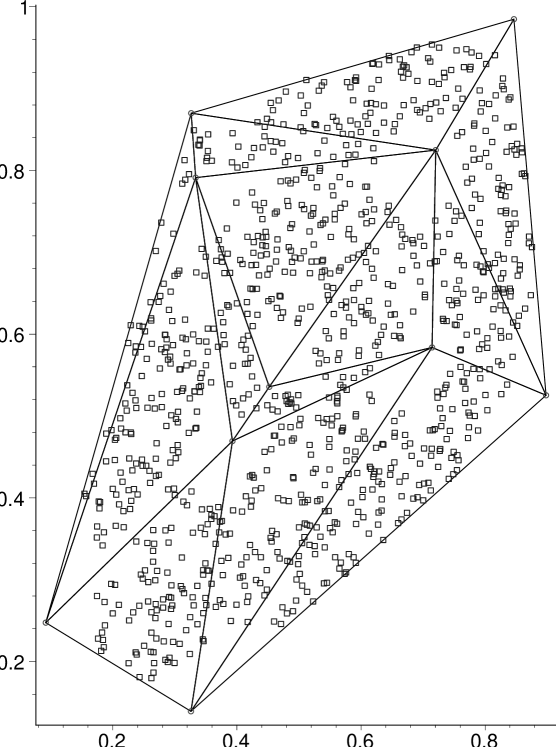
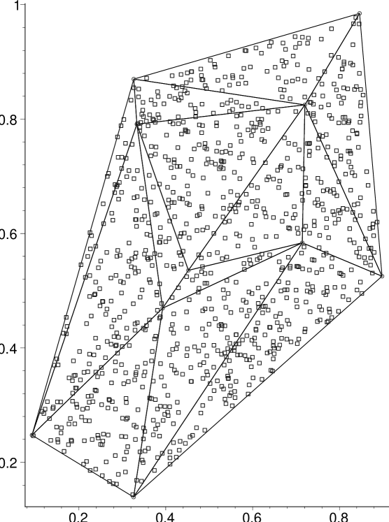
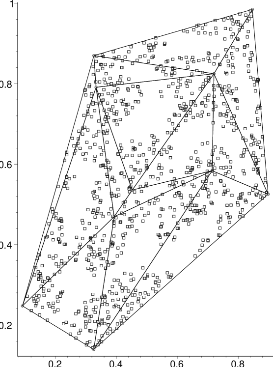
Figure 1: Realizations of segregation (left), CSR (middle), and association (right) for $|\mathcal{Y}|=10$ and $|\mathcal{X}|=1000$. $Y$ points are at the vertices of the triangles, and $X$ points are squares.

2 Spatial Point Patterns

For simplicity, we describe the spatial point patterns for two-class populations. The null hypothesis for spatial patterns have been a controversial topic in ecology from the early days (Gotelli and Graves, (1996)). But in general, the null hypothesis consists of two random pattern types: complete spatial randomness or random labeling.

Under complete spatial randomness (CSR) for a spatial point pattern $\{X(D),A(D)\in\mathbb{R}^{2}\}$ where $A(\cdot)$ denotes the area functional, we have

• given $n$ events in domain $D$, the events are an independent random sample from a uniform distribution on $D$;

• there is no spatial interaction.

Furthermore, the number of events in any planar region with area $A(D)$ follows a Poisson distribution with mean $\lambda\cdot A(D)$, whose probability mass function is given by

$$f_{X(D)}(x)=\frac{e^{-\lambda\cdot A(D)}(\lambda\cdot A(D))^{x}}{x!},\;\;x\in\{0,1,2,\ldots\}$$

where $\lambda$ is the intensity of the Poisson distribution.

Under random labeling, class labels are assigned to a fixed set of points randomly so that the labels are independent of the locations. Thus, random labeling is less restrictive than CSR. But conditional on a set of points from CSR, both processes are equivalent. We only consider a special case of CSR as our null hypothesis in this article. That is, only $X$ points are assumed to be uniformly distributed over the convex hull of $Y$ points.

The alternative patterns fall under two major categories called association and segregation. Association occurs if the points from the two classes together form clumps or clusters. That is, association occurs when members of one class have a tendency to attract members of the other class, as in symbiotic species, so that the $X_{i}$ will tend to cluster around the elements of $\mathcal{Y}$. For example, in plant biology, $\mathcal{X}$ points might be parasitic plants exploiting $\mathcal{Y}$ points. As another example, $\mathcal{X}$ and $\mathcal{Y}$ points might represent mutualistic plant species, so they depend on each other to survive. In epidemiology, $\mathcal{Y}$ points might be contaminant sources, such as a nuclear reactor, or a factory emitting toxic gases, and $\mathcal{X}$ points might be the residence of cases (incidences) of certain diseases caused by the contaminant, e.g., some type of cancer. Segregation occurs if the members of the same class tend to be clumped or clustered (see, e.g., Pielou, (1961)). Many different forms of segregation are possible. Our methods will be useful only for the segregation patterns in which the two classes more or less share the same support (habitat), and members of one class have a tendency to repel members of the other class. For instance, it may be the case that one type of plant does not grow well in the vicinity of another type of plant, and vice versa. This implies, in our notation, that $X_{i}$ are unlikely to be located near any elements of $\mathcal{Y}$. See, for instance, (Dixon, (1994); Coomes et al., (1999)). In plant biology, $\mathcal{Y}$ points might represent a tree species with a large canopy, so that, other plants ($\mathcal{X}$ points) that need light cannot grow around these trees. As another interesting but contrived example, consider the arsonist who wishes to start fires with maximum duration time (hence maximum damage), so that he starts the fires at the furthest points possible from fire houses in a city. Then $\mathcal{Y}$ points could be the fire houses, while $\mathcal{X}$ points will be the locations of arson cases.

We consider completely mapped data, i.e., the locations of all events in a defined space are observed rather than sparsely sampled data (only a random subset of locations are observed).

3 Data-Random Proximity Catch Digraphs

In general, in a random digraph, there is an arc between two vertices, with a fixed probability, independent of other arcs and vertex pairs. However, in our approach, arcs with a shared vertex will be dependent. Hence the name data-random digraphs.

Let $(\Omega,\mathcal{M})$ be a measurable space and consider a function $N:\Omega\times 2^{\Omega}\rightarrow 2^{\Omega}$, where $2^{\Omega}$ represents the power set of $\Omega$. Then given $\mathcal{Y}\subseteq\Omega$, the proximity map $N_{\mathcal{Y}}(\cdot)=N(\cdot,\mathcal{Y}):\Omega\rightarrow 2^{\Omega}$ associates a proximity region $N_{\mathcal{Y}}(x)\subseteq\Omega$ with each point $x\in\Omega$. The region $N_{\mathcal{Y}}(x)$ is defined in terms of the distance between $x$ and $\mathcal{Y}$.

If $\mathcal{X}_{n}:=\{X_{1},X_{2},\cdots,X_{n}\}$ is a set of $\Omega$-valued random variables, then the $N_{\mathcal{Y}}(X_{i}),\;i=1,\cdots,n$, are random sets. If the $X_{i}$ are independent and identically distributed, then so are the random sets, $N_{\mathcal{Y}}(X_{i})$.

Define the data-random proximity catch digraph $D$ with vertex set $\mathcal{V}=\{X_{1},\cdots,X_{n}\}$ and arc set $\mathcal{A}$ by $(X_{i},X_{j})\in\mathcal{A}\iff X_{j}\in N_{\mathcal{Y}}(X_{i})$ where point $X_{i}$ “catches” point $X_{j}$. The random digraph $D$ depends on the (joint) distribution of the $X_{i}$ and on the map $N_{\mathcal{Y}}$. The adjective proximity — for the catch digraph $D$ and for the map $N_{\mathcal{Y}}$ — comes from thinking of the region $N_{\mathcal{Y}}(x)$ as representing those points in $\Omega$ “close” to $x$ (Toussaint, (1980) and Jaromczyk and Toussaint, (1992)).

The relative density of a digraph $D=(\mathcal{V},\mathcal{A})$ of order $|\mathcal{V}|=n$ (i.e., number of vertices is $n$), denoted $\rho(D)$, is defined as

$$\rho(D)=\frac{|\mathcal{A}|}{n(n-1)}$$

where $|\cdot|$ denotes the set cardinality functional (Janson et al., (2000)).

Thus $\rho(D)$ represents the ratio of the number of arcs in the digraph $D$ to the number of arcs in the complete symmetric digraph of order $n$, namely $n(n-1)$.

If $X_{1},\cdots,X_{n}\stackrel{{\scriptstyle iid}}{{\sim}}F$, then the relative density of the associated data-random proximity catch digraph $D$, denoted $\rho(\mathcal{X}_{n};h,N_{\mathcal{Y}})$, is a U-statistic,

$$\rho(\mathcal{X}_{n};h,N_{\mathcal{Y}})=\frac{1}{n(n-1)}\sum\sum_{i<j\hskip 18.06749pt}h(X_{i},X_{j};N_{\mathcal{Y}})$$ (1)

where

$$h(X_{i},X_{j};N_{\mathcal{Y}}) = \mathbf{I}\{(X_{i},X_{j})\in\mathcal{A}\}+\mathbf{I}\{(X_{j},X_{i})\in\mathcal{A}\}$$ (2)

$$= \mathbf{I}\{X_{j}\in N_{\mathcal{Y}}(X_{i})\}+\mathbf{I}\{X_{i}\in N_{\mathcal{Y}}(X_{j})\}$$

with $\mathbf{I}(\cdot)$ being the indicator function. We denote $h(X_{i},X_{j};N_{\mathcal{Y}})$ as $h_{ij}$ henceforth for brevity of notation. Although the digraph is not symmetric (since $(x,y)\in\mathcal{A}$ does not necessarily imply $(y,x)\in\mathcal{A}$), $h_{ij}$ is defined as the number of arcs in $D$ between vertices $X_{i}$ and $X_{j}$, in order to produce a symmetric kernel with finite variance (Lehmann, (1988)).

The random variable $\rho_{n}:=\rho(\mathcal{X}_{n};h,N_{\mathcal{Y}})$ depends on $n$ and $N_{\mathcal{Y}}$ explicitly and on $F$ implicitly. The expectation $\mathbf{E}\,[\rho_{n}]$, however, is independent of $n$ and depends on only $F$ and $N_{\mathcal{Y}}$:

$$0\leq\mathbf{E}\,[\rho_{n}]=\frac{1}{2}\mathbf{E}\,[h_{12}]\leq 1\mbox{ for all $n\geq 2$}.$$ (3)

The variance $\mathbf{Var}\,[\rho_{n}]$ simplifies to

$$0\leq\mathbf{Var}\,[\rho_{n}]=\frac{1}{2n(n-1)}\mathbf{Var}\,[h_{12}]+\frac{n-2}{n(n-1)}\mathbf{Cov}\,[h_{12},h_{13}]\leq 1/4.$$ (4)

A central limit theorem for $U$-statistics (Lehmann, (1988)) yields

$$\sqrt{n}(\rho_{n}-\mathbf{E}\,[\rho_{n}])\stackrel{{\scriptstyle\mathcal{L}}}{{\longrightarrow}}\mathcal{N}(0,\mathbf{Cov}\,[h_{12},h_{13}])$$ (5)

provided that $\mathbf{Cov}\,[h_{12},h_{13}]>0$. The asymptotic variance of $\rho_{n}$, $\mathbf{Cov}\,[h_{12},h_{13}]$, depends on only $F$ and $N_{\mathcal{Y}}$. Thus, we need determine only $\mathbf{E}\,[h_{12}]$ and $\mathbf{Cov}\,[h_{12},h_{13}]$ in order to obtain the normal approximation

$$\rho_{n}\stackrel{{\scriptstyle\mbox{approx}}}{{\sim}}\mathcal{N}\left(\mathbf{E}\,[\rho_{n}],\mathbf{Var}\,[\rho_{n}]\right)=\mathcal{N}\left(\frac{\mathbf{E}\,[h_{12}]}{2},\frac{\mathbf{Cov}\,[h_{12},h_{13}]}{n}\right)\mbox{ for large $n$}.$$ (6)

3.1 The $\tau$-Factor Central Similarity Proximity Catch Digraphs

We define the $\tau$-factor central similarity proximity map briefly. Let $\Omega=\mathbb{R}^{2}$ and let $\mathcal{Y}=\{\mathsf{y}_{1},\mathsf{y}_{2},\mathsf{y}_{3}\}\subset\mathbb{R}^{2}$ be three non-collinear points. Denote the triangle — including the interior — formed by the points in $\mathcal{Y}$ as $T(\mathcal{Y})$. For $\tau\in[0,1]$, define $N_{\mathcal{Y}}^{\tau}$ to be the $\tau$-factor central similarity proximity map as follows; see also Figure 2. Let $e_{j}$ be the edge opposite vertex $\mathsf{y}_{j}$ for $j=1,2,3$, and let “edge regions” $R(e_{1})$, $R(e_{2})$, $R(e_{3})$ partition $T(\mathcal{Y})$ using segments from the center of mass of $T(\mathcal{Y})$ to the vertices. For $x\in T(\mathcal{Y})\setminus\mathcal{Y}$, let $e(x)$ be the edge in whose region $x$ falls; $x\in R(e(x))$. If $x$ falls on the boundary of two edge regions we assign $e(x)$ arbitrarily. For ${\tau}\in(0,1]$, the $\tau$-factor central similarity proximity region $N_{CS}^{\tau}(x)=N_{\mathcal{Y}}^{\tau}(x)$ is defined to be the triangle $T_{\tau}(x)$ with the following properties:

• $T_{\tau}(x)$ has an edge $e_{\tau}(x)$ parallel to $e(x)$ such that $d(x,e_{\tau}(x))=\tau\,d(x,e(x))$ and $d(e_{\tau}(x),e(x))\leq d(x,e(x))$ where $d(x,e(x))$ is the Euclidean (perpendicular) distance from $x$ to $e(x)$,

• $T_{\tau}(x)$ has the same orientation as and is similar to $T(\mathcal{Y})$,

• $x$ is at the center of mass of $T_{\tau}(x)$.

Note that (i) implies the “$\tau$-factor”, (ii) implies “similarity”, and (iii) implies “central” in the name, $\tau$-factor central similarity proximity map. Notice that $\tau>0$ implies that $x\in N_{CS}^{\tau}(x)$ and $\tau\leq 1$ implies that $N_{CS}^{\tau}(x)\subseteq T(\mathcal{Y})$ for all $x\in T(\mathcal{Y})$. For $x\in\partial(T(\mathcal{Y}))$ and $\tau\in[0,1]$, we define $N_{CS}^{\tau}(x)=\{x\}$; for $\tau=0$ and $x\in T(\mathcal{Y})$ we also define $N_{CS}^{\tau}(x)=\{x\}$. Let $T(\mathcal{Y})^{o}$ be the interior of the triangle $T(\mathcal{Y})$. Then for all $x\in T(\mathcal{Y})^{o}$ the edges $e_{\tau}(x)$ and $e(x)$ are coincident iff $\tau=1$. Observe that the central similarity proximity map in (Ceyhan and Priebe, (2003)) is $N_{CS}^{\tau}(\cdot)$ with $\tau=1$. Hence by definition, $(x,y)$ is an arc of the $\tau$-factor central similarity PCD iff $y\in N_{CS}^{\tau}(x)$.

Notice that $X_{i}\stackrel{{\scriptstyle iid}}{{\sim}}F$, with the additional assumption that the non-degenerate two-dimensional probability density function $f$ exists with support in $T(\mathcal{Y})$, implies that the special case in the construction of $N_{CS}^{\tau}$ — $X$ falls on the boundary of two edge regions — occurs with probability zero.

Figure 2: Construction of $\tau$-factor central similarity proximity region, $N_{CS}^{1/2}(x)$ (shaded region).

For a fixed $\tau\in(0,1]$, $N_{CS}^{\tau}(x)$ gets larger (in area) as $x$ gets further away from the edges (or equivalently gets closer to the center of mass, $C_{M}$) in the sense that as $d(x,e(x))$ increases (or equivalently $d(C_{M},e_{\tau}(x))$ decreases. Hence for points in $T(\mathcal{Y})$, the further the points away from the vertices $\mathcal{Y}$ (or closer the points to $C_{M}$ in the above sense), the larger the area of $N_{CS}^{\tau}(x)$. Hence, it is more likely for such points to catch other points, i.e., have more arcs directed to other points. Therefore, if more $X$ points are clustered around the center of mass, then the digraph is more likely to have more arcs, hence larger relative density. So, under segregation, relative density is expected to be larger than that in CSR or association. On the other hand, in the case of association, i.e., when $X$ points are clustered around $Y$ points, the regions $N_{CS}^{\tau}(x)$ tend to be smaller in area, hence, catch less points, thereby resulting in a small number of arcs, or a smaller relative density compared to CSR or segregation. See, for example, Figure 3 with 3 $Y$ points, and 20 $X$ points for segregation (top left), CSR (middle left) and association (bottom right). The corresponding arcs in the $\tau$-factor central similarity PCD with $\tau=1$ are plotted in the right in Figure 3. The corresponding relative density values (for $\tau=1$) are .1395, .2579, and .0974, respectively.

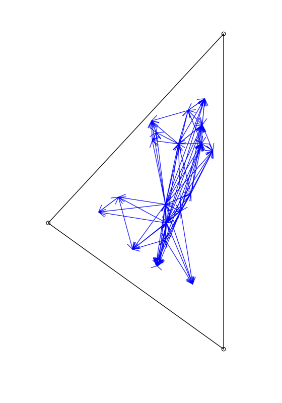
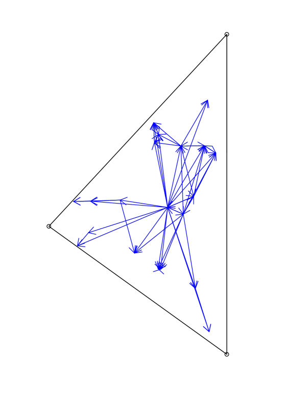
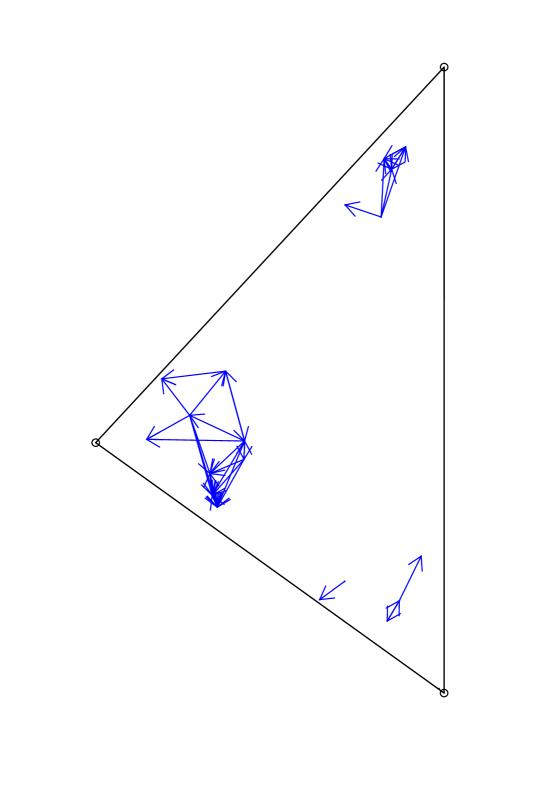
Figure 3: Realizations of segregation (left), CSR (middle), and association (right) for $|\mathcal{Y}|=3$ and $|\mathcal{X}|=20$. $Y$ points are at the vertices of the triangle, and $X$ points are squares. The number of arcs with $\tau=1$ are 98, 53, and 37, respectively. So, relative density values are .258, .139, and .097, respectively.

Furthermore, for a fixed $x\in T(\mathcal{Y})^{o}$, $N_{CS}^{\tau}(x)$ gets larger (in area) as $\tau$ increases. So, as $\tau$ increases, it is more likely to have more arcs, hence larger relative density for a given realization of $\mathcal{X}$ points in $T(\mathcal{Y})$.

4 Asymptotic Distribution of the Relative Density

We first describe the null and alternative patterns we consider briefly, and then provide the asymptotic distribution of the relative density for these patterns.

There are two major types of asymptotic structures for spatial data (Lahiri, (1996)). In the first, any two observations are required to be at least a fixed distance apart, hence as the number of observations increase, the region on which the process is observed eventually becomes unbounded. This type of sampling structure is called “increasing domain asymptotics”. In the second type, the region of interest is a fixed bounded region and more and more points are observed in this region. Hence the minimum distance between data points tends to zero as the sample size tends to infinity. This type of structure is called “infill asymptotics”, due to Cressie, (1991). The sampling structure for our asymptotic analysis is infill, as only the size of the type $X$ process tends to infinity, while the support, the convex hull of a given set of points from type $Y$ process, $C_{H}(\mathcal{Y})$ is a fixed bounded region.

4.1 Null and Alternative Patterns

For statistical testing for segregation and association, the null hypothesis is generally some form of complete spatial randomness; thus we consider

$$H_{o}:X_{i}\stackrel{{\scriptstyle iid}}{{\sim}}\mathcal{U}(T(\mathcal{Y})).$$

If it is desired to have the sample size be a random variable, we may consider a spatial Poisson point process on $T(\mathcal{Y})$ as our null hypothesis.

Geometry Invariance Property

We first present a “geometry invariance” result that will simplify our calculations by allowing us to consider the special case of the equilateral triangle.

Theorem 1: Let $\mathcal{Y}=\{\mathsf{y}_{1},\mathsf{y}_{2},\mathsf{y}_{3}\}\subset\mathbb{R}^{2}$ be three non-collinear points. For $i=1,\cdots,n$ let $X_{i}\stackrel{{\scriptstyle iid}}{{\sim}}F=\mathcal{U}(T(\mathcal{Y}))$, the uniform distribution on the triangle $T(\mathcal{Y})$. Then for any $\tau\in[0,1]$ the distribution of $\rho_{n}(\tau):=\rho(\mathcal{X}_{n};h,N_{CS}^{\tau})$ is independent of $\mathcal{Y}$, hence the geometry of $T(\mathcal{Y})$.

Based on Theorem 1 and our uniform null hypothesis, we may assume that $T(\mathcal{Y})$ is the standard equilateral triangle with $\mathcal{Y}=\bigl{\{}(0,0),(1,0),\bigl{(}1/2,\sqrt{3}/2\bigr{)}\bigr{\}}$, henceforth. For our $\tau$-factor central similarity proximity map and uniform null hypothesis, the asymptotic null distribution of $\rho_{n}(\tau)=\rho(\mathcal{X}_{n};h,N_{CS}^{\tau})$ as a function of $\tau$ can be derived. Let $\mu(\tau):=\mathbf{E}\,[\rho_{n}]$, then $\mu(\tau)=\mathbf{E}\,[h_{12}]/2=P(X_{2}\in N_{CS}^{\tau}(X_{1}))$ is the probability of an arc occurring between any two vertices and let $\nu(\tau):=\mathbf{Cov}\,[h_{12},h_{13}]$.

We define two simple classes of alternatives, $H^{S}_{\varepsilon}$ and $H^{A}_{\varepsilon}$ with $\varepsilon\in\bigl{(}0,\sqrt{3}/3\bigr{)}$, for segregation and association, respectively. See also Figure 4. For $\mathsf{y}\in\mathcal{Y}$, let $e(\mathsf{y})$ denote the edge of $T(\mathcal{Y})$ opposite vertex $\mathsf{y}$, and for $x\in T(\mathcal{Y})$ let $\ell_{\mathsf{y}}(x)$ denote the line parallel to $e(\mathsf{y})$ through $x$. Then define $T(\mathsf{y},\varepsilon)=\bigl{\{}x\in T(\mathcal{Y}):d(\mathsf{y},\ell_{\mathsf{y}}(x))\leq\varepsilon\bigr{\}}$. Let $H^{S}_{\varepsilon}$ be the model under which $X_{i}\stackrel{{\scriptstyle iid}}{{\sim}}\mathcal{U}\Bigl{(}T(\mathcal{Y})\setminus\cup_{\mathsf{y}\in\mathcal{Y}}T(\mathsf{y},\varepsilon)\Bigr{)}$ and $H^{A}_{\varepsilon}$ be the model under which $X_{i}\stackrel{{\scriptstyle iid}}{{\sim}}\mathcal{U}\Bigl{(}\cup_{\mathsf{y}\in\mathcal{Y}}T\bigl{(}\mathsf{y},\sqrt{3}/3-\varepsilon\bigr{)}\Bigr{)}$. The shaded region in Figure 4 is the support for segregation for a particular $\varepsilon$ value; and its complement is the support for the association alternative with $\sqrt{3}/3-\varepsilon$. Thus the segregation model excludes the possibility of any $X_{i}$ occurring near a $\mathsf{y}_{j}$, and the association model requires that all $X_{i}$ occur near a $\mathsf{y}_{j}$. The $\sqrt{3}/3-\varepsilon$ in the definition of the association alternative is so that $\varepsilon=0$ yields $H_{o}$ under both classes of alternatives. We consider these types of alternatives among many other possibilities, since relative density is geometry invariant for these alternatives as the alternatives are defined with parallel lines to the edges.

Figure 4: An example for the segregation alternative for a particular $\varepsilon$ (shaded region), and its complement is for the association alternative (unshaded region) on the standard equilateral triangle.

Remark: These definitions of the alternatives are given for the standard equilateral triangle. The geometry invariance result of Theorem 1 from Section 4 still holds under the alternatives, in the following sense. If, in an arbitrary triangle, a small percentage $\delta\cdot 100\%$ where $\delta\in(0,4/9)$ of the area is carved away as forbidden from each vertex using line segments parallel to the opposite edge, then under the transformation to the standard equilateral triangle this will result in the alternative $H^{S}_{\sqrt{3\delta/4}}$. This argument is for segregation with $\delta<1/4$; a similar construction is available for the other cases.

4.2 Asymptotic Normality Under the Null Hypothesis

By detailed geometric probability calculations provided in the Appendix, the mean and the asymptotic variance of the relative density of the $\tau$-factor proximity catch digraph can be calculated explicitly. The central limit theorem for $U$-statistics then establishes the asymptotic normality under the uniform null hypothesis. These results are summarized in the following theorem.

Theorem 2: For $\tau\in(0,1]$, the relative density of the $\tau$-factor central similarity proximity digraph converges in law to the normal distribution, i.e., as $n\rightarrow\infty$,

$$\frac{\sqrt{n}(\rho_{n}(\tau)-\mu(\tau))}{\sqrt{\nu(\tau)}}\stackrel{{\scriptstyle\mathcal{L}}}{{\longrightarrow}}\mathcal{N}(0,1)$$ (7)

where

$$\mu(\tau)=\tau^{2}/6$$ (8)

and

$$\nu(\tau)=\frac{\tau^{4}(6\,\tau^{5}-3\,\tau^{4}-25\,\tau^{3}+\tau^{2}+49\,\tau+14)}{45\,(\tau+1)(2\,\tau+1)(\tau+2)}$$ (9)

For $\tau=0$, $\rho_{n}(\tau)$ is degenerate for all $n>1$.

See the Appendix for the derivation.

Consider the form of the mean and the variance functions, which are depicted in Figure 5. Note that $\mu(\tau)$ is monotonically increasing in $\tau$, since $N_{CS}^{\tau}(x)$ increases with $\tau$ for all $x\in T(\mathcal{Y})^{o}$. Note also that $\mu(\tau)$ is continuous in $\tau$ with $\mu(\tau=1)=1/6$ and $\mu(\tau=0)=0$.

Regarding the asymptotic variance, note that $\nu(\tau)$ is continuous in $\tau$ and $\nu(\tau=1)=7/135$ and $\nu(\tau=0)=0$ —there are no arcs when $\tau=0$ a.s.— which explains why $\rho_{n}(\tau=0)$ is degenerate.

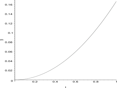
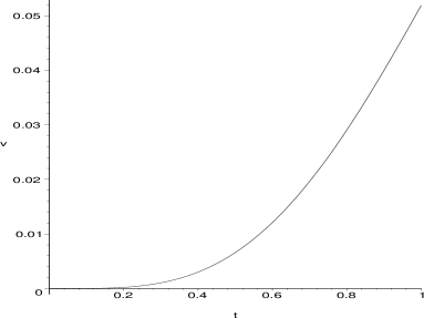
Figure 5: Result of Theorem 2: asymptotic null mean $\mu(\tau)=\mu(\tau)$ (left) and variance $\nu(\tau)=\nu(\tau)$ (right), from Equations (8) and (9), respectively.

As an example of the limiting distribution, $\tau=1/2$ yields

$$\frac{\sqrt{n}\bigl{(}\rho_{n}(1/2)-\mu(1/2)\bigr{)}}{\sqrt{\nu(1/2)}}=\sqrt{\frac{2880\,n}{19}}\bigl{(}\rho_{n}(1/2)-1/24\bigr{)}\stackrel{{\scriptstyle\mathcal{L}}}{{\longrightarrow}}\mathcal{N}(0,1)$$

or equivalently,

$$\rho_{n}(1/2)\stackrel{{\scriptstyle\mbox{\tiny{approx}}}}{{\sim}}\mathcal{N}\left(\frac{1}{24},\frac{19}{2880\,n}\right).$$

The finite sample variance and skewness may be derived analytically in much the same way as was $\mathbf{Cov}\,[h_{12},h_{13}]$ for the asymptotic variance. In fact, the exact distribution of $\rho_{n}(\tau)$ is, in principle, available by successively conditioning on the values of the $X_{i}$. Alas, while the joint distribution of $h_{12},h_{13}$ is available, the joint distribution of $\{h_{ij}\}_{1\leq i<j\leq n}$, and hence the calculation for the exact distribution of $\rho_{n}(\tau)$, is extraordinarily tedious and lengthy for even small values of $n$.

Figure 6 indicates that, for $\tau=1/2$, the normal approximation is accurate even for small $n$ (although kurtosis and skewness may be indicated for $n=10,\,20$). Figure 7 demonstrates, however, that the smaller the value of $\tau$ the more severe the skewness of the probability density.

\psfrag{Density}{ \Huge{\bf{density}}}\includegraphics{CSnormskewa.ps}

\psfrag{Density}{ \Huge{\bf{density}}}\includegraphics{CSnormskewb.ps}

\psfrag{Density}{ \Huge{\bf{density}}}\includegraphics{CSnormskewc.ps}

Figure 6: Depicted are $\rho_{n}(1/2)\stackrel{{\scriptstyle\mbox{approx}}}{{\sim}}\mathcal{N}\left(\frac{1}{24},\frac{19}{2880\,n}\right)$ for $n=10,\,20,\,100$ (left to right). Histograms are based on 1000 Monte Carlo replicates. Solid curves represent the approximating normal densities given in Theorem 2. Note that the vertical axes are differently scaled.

\psfrag{Density}{ \Huge{\bf{density}}}\includegraphics{CSskewn10d1.ps}

\psfrag{Density}{ \Huge{\bf{density}}}\includegraphics{CSskewn10d2.ps}

\psfrag{Density}{ \Huge{\bf{density}}}\includegraphics{CSskewn10d3.ps}

Figure 7: Depicted are the histograms for 10000 Monte Carlo replicates of $\rho_{10}(1/4)$ (left), $\rho_{10}(3/4)$ (middle), and $\rho_{10}(1)$ (right) indicating severe small sample skewness for small values of $\tau$.

4.3 Asymptotic Normality Under the Alternatives

Asymptotic normality of the relative density of the proximity catch digraph can be established under the alternative hypotheses of segregation and association by the same method as under the null hypothesis. Let $\mathbf{E}\,_{\varepsilon}[\cdot]$ be the expectation with respect to the uniform distribution under the segregation and association alternatives with $\varepsilon\in\bigl{(}0,\sqrt{3}/3\bigr{)}$.

Theorem 3: Let $\mu_{S}(\tau,\varepsilon)$ ( $\mu_{A}(\tau,\varepsilon)$ ) be the mean and $\nu_{S}(\tau,\varepsilon)$ ( $\nu_{A}(\tau,\varepsilon)$ ) be the covariance, $\mathbf{Cov}\,[h_{12},h_{13}]$ for $\tau\in(0,1]$ and $\varepsilon\in\bigl{(}0,\sqrt{3}/3\bigr{)}$ under segregation ( association ). Then under $H^{S}_{\varepsilon}$, $\sqrt{n}\bigl{(}\rho_{n}(\tau)-\mu_{S}(\tau,\varepsilon)\bigr{)}\stackrel{{\scriptstyle\mathcal{L}}}{{\longrightarrow}}\mathcal{N}\bigl{(}0,\nu_{S}(\tau,\varepsilon)\bigr{)}$ for the values of the pair $(\tau,\varepsilon)$ for which $\nu_{S}(\tau,\varepsilon)>0$. $\rho_{n}(\tau)$ is degenerate when $\nu_{S}(\tau,\varepsilon)=0$. Likewise, under $H^{A}_{\varepsilon}$, $\sqrt{n}\bigl{(}\rho_{n}(\tau)-\mu_{A}(\tau,\varepsilon)\bigr{)}\stackrel{{\scriptstyle\mathcal{L}}}{{\longrightarrow}}\mathcal{N}\bigl{(}0,\nu_{A}(\tau,\varepsilon)\bigr{)}$ for the values of the pair $(\tau,\varepsilon)$ for which $\nu_{A}(\tau,\varepsilon)>0$. $\rho_{n}(\tau)$ is degenerate when $\nu_{A}(\tau,\varepsilon)=0$.

Notice that under the association alternatives any $\tau\in(0,1]$ yields asymptotic normality for all $\varepsilon\in\bigl{(}0,\sqrt{3}/3\bigr{)}$, while under the segregation alternatives only $\tau=1$ yields this universal asymptotic normality.

5 The Test and Analysis

The relative density of the central similarity proximity catch digraph is a test statistic for the segregation/association alternative; rejecting for extreme values of $\rho_{n}(\tau)$ is appropriate since under segregation, we expect $\rho_{n}(\tau)$ to be large; while under association, we expect $\rho_{n}(\tau)$ to be small. Using the test statistic

$$R(\tau)=\frac{\sqrt{n}\bigl{(}\rho_{n}(\tau)-\mu(\tau)\bigr{)}}{\sqrt{\nu(\tau)}},$$ (10)

which is the normalized relative density, the asymptotic critical value for the one-sided level $\alpha$ test against segregation is given by

$$z_{\alpha}=\Phi^{-1}(1-\alpha).$$

Against segregation, the test rejects for $R(\tau)>z_{\alpha}$ and against association, the test rejects for $R(\tau)<z_{1-\alpha}$. For the example patterns in Figure 3, $R(\tau=1)=1.792,-.534$, and -1.361, respectively.

5.1 Consistency of the Tests Under the Alternatives

Theorem 4: The test against $H^{S}_{\varepsilon}$ which rejects for $R(\tau)>z_{\alpha}$ and the test against $H^{A}_{\varepsilon}$ which rejects for $R(\tau)<z_{1-\alpha}$ are consistent for $\tau\in(0,1]$ and $\varepsilon\in\bigl{(}0,\sqrt{3}/3\bigr{)}$.

In fact, the analysis of the means under the alternatives reveals more than what is required for consistency. Under segregation, the analysis indicates that $\mu_{S}(\tau,\varepsilon_{1})<\mu_{S}(\tau,\varepsilon_{2})$ for $\varepsilon_{1}<\varepsilon_{2}$. On the other hand, under association, the analysis indicates that $\mu_{A}(\tau,\varepsilon_{1})>\mu_{A}(\tau,\varepsilon_{2})$ for $\varepsilon_{1}<\varepsilon_{2}$.

5.2 Monte Carlo Power Analysis

In this section, we asses the finite sample behaviour of the relative density using Monte Carlo simulations for testing CSR against segregation or association. We provide the kernel density estimates, empirical significance levels, and empirical power estimates under the null case and various segregation and association alternatives.

5.2.1 Monte Carlo Power Analysis for Segregation Alternatives

In Figures 8 and 9, we present the kernel density estimates under $H_{o}$ and $H^{S}_{\varepsilon}$ with $\varepsilon=\sqrt{3}/8,\,\sqrt{3}/4,\,2\,\sqrt{3}/7$. Observe that with $n=10$, and $\varepsilon=\sqrt{3}/8$, the density estimates are very similar implying small power; and as $\varepsilon$ gets larger, the separation between the null and alternative curves gets larger, hence the power gets larger. With $n=10$, 10000 Monte Carlo replicates yield power estimates $\widehat{\beta}^{S}_{mc}(\varepsilon)=.0994,\,.9777,\,1.000$, respectively. With $n=100$, there is more separation between the null and alternative curves at each $\varepsilon$, which implies that power increases as $\varepsilon$ increases. With $n=100$, 1000 Monte Carlo replicates yield $\widehat{\beta}^{S}_{mc}(\varepsilon)=.5444,\,1.000,\,1.000$.

\psfrag{kernel density estimate}{ \Huge{\bf{kernel density estimate}}}\psfrag{relative density}{ \Huge{\bf{relative density}}}\includegraphics{CSsegsim5.ps}

\psfrag{kernel density estimate}{ \Huge{\bf{kernel density estimate}}}\psfrag{relative density}{ \Huge{\bf{relative density}}}\includegraphics{CSseg2sim5.ps}

\psfrag{kernel density estimate}{ \Huge{\bf{kernel density estimate}}}\psfrag{relative density}{ \Huge{\bf{relative density}}}\includegraphics{CSseg3sim5.ps}

Figure 8: Kernel density estimates for the null (solid) and the segregation alternative $H^{S}_{\varepsilon}$ (dashed) with $\tau=1/2$, $n=10$, $N=10000$, and $\varepsilon=\sqrt{3}/8$ (left), $\varepsilon=\sqrt{3}/4$ (middle), and $\varepsilon=2\,\sqrt{3}/7$ (right).

\psfrag{kernel density estimate}{ \Huge{\bf{kernel density estimate}}}\psfrag{relative density}{ \Huge{\bf{relative density}}}\includegraphics{CSsegsim5n100.ps}

\psfrag{kernel density estimate}{ \Huge{\bf{kernel density estimate}}}\psfrag{relative density}{ \Huge{\bf{relative density}}}\includegraphics{CSseg2sim5n100.ps}

Figure 9: Kernel density estimates for the null (solid) and the segregation alternative $H^{S}_{\sqrt{3}/4}$ (dashed) for $\tau=1/2$ with $n=10$ and $N=10000$ (left) and $n=100$ and $N=1000$ (right).

For a given alternative and sample size, we may consider analyzing the power of the test — using the asymptotic critical value (i.e., the normal approximation)— as a function of $\tau$. Figure 10 presents a Monte Carlo investigation of power against $H^{S}_{\sqrt{3}/8}$, $H^{S}_{\sqrt{3}/4}$ as a function of $\tau$ for $n=10$. The corresponding empirical significance levels and power estimates are presented in Table 2. The empirical significance levels, $\widehat{\alpha}_{n=10}$, are all greater than $.05$ with smallest being $.0868$ at $\tau=1.0$ which have the empirical power $\widehat{\beta}_{10}(\sqrt{3}/8)=.2289$, $\widehat{\beta}_{10}(\sqrt{3}/4)=.9969$. However, the empirical significance levels imply that $n=10$ is not large enough for normal approximation. Notice that as $n$ gets larger, the empirical significance levels gets closer to $.05$ (except for $\tau=0.1$), but still are all greater than $.05$, which indicates that for $n\leq 100$, the test is liberal in rejecting $H_{o}$ against segregation. Furthermore, as $n$ increases, for fixed $\varepsilon$ the empirical power estimates increase, the empirical significance levels get closer to $.05$; and for fixed $n$ as $\tau$ increases power estimates get larger. Therefore, for segregation, we recommend the use of large $\tau$ values ($\tau\lesssim 1.0$).

\psfrag{power}{ \Huge{\bf{power}}}\includegraphics{CSsegtilde1.ps}

\psfrag{power}{ \Huge{\bf{power}}}\includegraphics{CSsegtilde2.ps}

Figure 10: Monte Carlo power using the asymptotic critical value against segregation alternatives $H^{S}_{\sqrt{3}/8}$ (left), $H^{S}_{\sqrt{3}/4}$ (right), as a function of $\tau$, for $n=10$ and $N=10000$. The circles represent the empirical significance levels while triangles represent the empirical power values.

$\tau$	.1	.2	.3	.4	.5	.6	.7	.8	.9	1.0
$n=10$, $N=10000$
$\widehat{\alpha}_{S}(n)$	.0932	.1916	.1740	.1533	.1101	.0979	.1035	.0945	.0883	.0868
$\widehat{\beta}^{S}_{n}(\tau,\sqrt{3}/8)$	.1286	.2630	.2917	.2811	.2305	.2342	.2526	.2405	.2334	.2289
$\widehat{\beta}^{S}_{n}(\tau,\sqrt{3}/4)$	.5821	.9011	.9824	.9945	.9967	.9979	.9990	.9985	.9983	.9969
$n=20$, $N=10000$
$\widehat{\alpha}_{S}(n)$	.2018	.1707	.1151	.1099	.0898	.0864	.0866	.0800	.0786	.0763
$\widehat{\beta}^{S}_{n}(\tau,\sqrt{3}/8)$	.2931	.3245	.2744	.3021	.2844	.2926	.3117	.3113	.3119	.3038
$n=100$, $N=1000$
$\widehat{\alpha}_{S}(n)$	.155	.101	.080	.077	.075	.066	.065	.063	.066	.069
$\widehat{\beta}^{S}_{n}(\tau,\sqrt{3}/8)$	.574	.574	.612	.655	.709	.742	.774	.786	.793	.793

Table 1: The empirical significance level and empirical power values under $H^{S}_{\varepsilon}$ for $\varepsilon=\sqrt{3}/8,\,\sqrt{3}/4$ at $\alpha=.05$.

5.2.2 Monte Carlo Power Analysis for Association Alternatives

In Figures 11 and 12, we present the kernel density estimates under $H_{o}$ and $H^{A}_{\varepsilon}$ with $\varepsilon=\sqrt{3}/21,\,\sqrt{3}/12,\,5\,\sqrt{3}/24$. Observe that with $n=10$, the density estimates are very similar for all $\varepsilon$ values (with slightly more separation for larger $\varepsilon$) implying small power. 10000 Monte Carlo replicates yield power estimates $\widehat{\beta}^{A}_{mc}\approx 0$. With $n=100$, there is more separation between the null and alternative curves at each $\varepsilon$, which implies that power increases as $\varepsilon$ increases. 1000 Monte Carlo replicates yield $\widehat{\beta}^{A}_{mc}=.324,\,.634,\,.634$, respectively.

\psfrag{kernel density estimate}{ \Huge{\bf{kernel density estimate}}}\psfrag{relative density}{ \Huge{\bf{relative density}}}\includegraphics{CSagg3sim5.ps}

\psfrag{kernel density estimate}{ \Huge{\bf{kernel density estimate}}}\psfrag{relative density}{ \Huge{\bf{relative density}}}\includegraphics{CSagg2sim5.ps}

\psfrag{kernel density estimate}{ \Huge{\bf{kernel density estimate}}}\psfrag{relative density}{ \Huge{\bf{relative density}}}\includegraphics{CSaggsim5.ps}

Figure 11: Kernel density estimates for the null (solid) and the association alternative $H^{A}_{\varepsilon}$ (dashed) for $\tau=1/2$ with $n=10$, $N=10000$ and $\varepsilon=\sqrt{3}/21$ (left), $\varepsilon=\sqrt{3}/12$ (middle), $\varepsilon=5\,\sqrt{3}/24$ (right).

For a given alternative and sample size, we may consider analyzing the power of the test — using the asymptotic critical value— as a function of $\tau$.

\psfrag{kernel density estimate}{ \Huge{\bf{kernel density estimate}}}\psfrag{relative density}{ \Huge{\bf{relative density}}}\includegraphics{CSagg3sim5n100.ps}

\psfrag{kernel density estimate}{ \Huge{\bf{kernel density estimate}}}\psfrag{relative density}{ \Huge{\bf{relative density}}}\includegraphics{CSagg2sim5n100.ps}

Figure 12: Kernel density estimates for the null (solid) and the association alternative $H^{A}_{\varepsilon}$ (dashed) for $\tau=1/2$ with $n=100$, $N=1000$ and $\varepsilon=\sqrt{3}/21$ (left), $\varepsilon=\sqrt{3}/12$ (right).

The empirical significance levels and power estimates against $H^{A}_{\varepsilon}$, with $\varepsilon=\sqrt{3}/12,\,5\,\sqrt{3}/24$ as a function of $\tau$ for $n=10$ are presented in Table 2. The empirical significance level closest to $.05$ occurs at $\tau=.6$, (much smaller for other $\tau$ values) which have the empirical power $\widehat{\beta}_{10}(\sqrt{3}/12)=.1181$, and $\widehat{\beta}_{10}(5\,\sqrt{3}/24)=.1187$. However, the empirical significance levels imply that $n=10$ is not large enough for normal approximation. With $n=20$, the empirical significance levels gets closer to $.05$ for $\tau=.3,\,.4,\,.5,\,.7,\,.8,\,.9,\,1.0$, with closest at $\tau=.4$ which has the empirical power $.1497$. With $n=100$, the empirical significance levels are $\approx.05$ for $\tau\geq.3$ and the highest empirical power is $.997$ at $\tau=1.0$. Note that as $n$ increases, the empirical power estimates increase for $\tau\geq.2$ and the empirical significance levels get closer to $.05$ for $\tau\geq.5$. This analysis indicate that in the one triangle case, the sample size should be really large ($n\geq 100$) for the normal approximation to be appropriate. Moreover, the smaller the $\tau$ value, the larger the sample needed for the normal approximation to be appropriate. Therefore, we recommend the use of large $\tau$ values ($\tau\lesssim 1.0$) for association.

$\tau$	.1	.2	.3	.4	.5	.6	.7	.8	.9	1.0
$n=10$, $N=10000$
$\widehat{\alpha}_{A}(n)$	0	0	0	0	0	.0465	.0164	.0223	.0209	.0339
$\widehat{\beta}^{A}_{n}(\tau,\sqrt{3}/12)$	0	0	0	0	0	.1181	.0569	.0831	.0882	.1490
$\widehat{\beta}^{A}_{n}(\tau,5\,\sqrt{3}/24)$	0	0	0	0	0	.1187	.0581	.0863	.0985	.1771
$n=20$, $N=10000$
$\widehat{\alpha}_{A}(n)$	.6603	.2203	.1069	.0496	.0338	.0301	.0290	.0267	.0333	.0372
$\widehat{\beta}^{A}_{n}(\tau,\sqrt{3}/12)$	.7398	.3326	.2154	.1497	.1442	.1608	.1818	.2084	.2663	.3167
$n=100$, $N=1000$
$\widehat{\alpha}_{A}(n)$	.169	.075	.053	.047	.049	.044	.040	.044	.049	.049
$\widehat{\beta}^{A}_{n}(\tau,\sqrt{3}/12)$	.433	.399	.460	.559	.687	.789	.887	.938	.977	.997

Table 2: The empirical significance level and empirical power values under $H^{A}_{\varepsilon}$ for $\varepsilon=5\,\sqrt{3}/24$, $\sqrt{3}/12$, $\sqrt{3}/21$ with $N=10000$, and $n=10$ at $\alpha=.05$.

5.2.3 Pitman Asymptotic Efficiency Under the Alternatives

Pitman asymptotic efficiency (PAE) provides for an investigation of “local asymptotic power” — local around $H_{o}$. This involves the limit as $n\rightarrow\infty$, as well as the limit as $\varepsilon\rightarrow 0$. See proof of Theorem 3 for the ranges of $\tau$ and $\varepsilon$ for which relative density is continuous as $n$ goes to $\infty$. A detailed discussion of PAE can be found in (Kendall and Stuart, (1979); Eeden, (1963). For segregation or association alternatives the PAE is given by $\mbox{PAE}(\rho_{n}(\tau))=\frac{\left(\mu^{(k)}(\tau,\varepsilon=0)\right)^{2}}{\nu(\tau)}$ where $k$ is the minimum order of the derivative with respect to $\varepsilon$ for which $\mu^{(k)}(\tau,\varepsilon=0)\not=0$. That is, $\mu^{(k)}(r,\varepsilon=0)\not=0$ but $\mu^{(l)}(\tau,\varepsilon=0)=0$ for $l=1,2,\ldots,k-1$. Then under segregation alternative $H^{S}_{\varepsilon}$ and association alternative $H^{A}_{\varepsilon}$, the PAE of $\rho_{n}(\tau)$ is given by

$$\mbox{PAE}^{S}(\tau)=\frac{\left(\mu^{\prime\prime}_{S}(\tau,\varepsilon=0)\right)^{2}}{\nu(\tau)}\mbox{ and }\mbox{PAE}^{A}(\tau)=\frac{\left(\mu^{\prime\prime}_{A}(\tau,\varepsilon=0)\right)^{2}}{\nu(\tau)},$$

respectively, since $\mu_{S}^{\prime}(\tau,\varepsilon=0)=\mu_{A}^{\prime}(\tau,\varepsilon=0)=0$. Equation (9) provides the denominator; the numerator requires $\mu_{S}(\tau,\varepsilon)$ and $\mu_{A}(\tau,\varepsilon)$ which are provided in the Appendix, where we only use the intervals of $\tau$ that do not vanish as $\varepsilon\rightarrow 0$.

In Figure 13, we present the PAE as a function of $\tau$ for both segregation and association.

Notice that $\lim_{\tau\rightarrow 0}\mbox{PAE}^{S}(\tau)=320/7\approx 45.7143$, $\mbox{argsup}_{\tau\in(0,1]}\mbox{PAE}^{S}(\tau)=1.0$, and $\mbox{PAE}^{S}(\tau=1)=960/7\approx 137.1429$. Based on the PAE analysis, we suggest, for large $n$ and small $\varepsilon$, choosing $\tau$ large (i.e., $\tau=1$) for testing against segregation.

Notice that $\lim_{\tau\rightarrow 0}\mbox{PAE}^{A}(\tau)=72000/7\approx 10285.7143$, $\mbox{PAE}^{A}(\tau=1)=61440/7\approx 8777.1429$, $\mbox{arginf}_{\tau\in(0,1]}\mbox{PAE}^{A}(\tau)\approx.4566$ with $\mbox{PAE}^{A}(\tau\approx.4566)\approx 6191.0939$. Based on the asymptotic efficiency analysis, we suggest, for large $n$ and small $\varepsilon$, choosing $\tau$ small for testing against association. However, for small and moderate values of $n$ the normal approximation is not appropriate due to the skewness in the density of $\rho_{n}(\tau)$. Therefore, for small and moderate $n$, we suggest large $\tau$ values ($\tau\lesssim 1$).

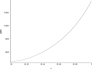
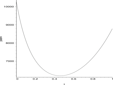
Figure 13: Pitman asymptotic efficiency against segregation (left) and association (right) as a function of $\tau$.

5.3 The Case with Multiple Delaunay Triangles

Suppose $\mathcal{Y}$ is a finite collection of points in $\mathbb{R}^{2}$ with $|\mathcal{Y}|\geq 3$. Consider the Delaunay triangulation (assumed to exist) of $\mathcal{Y}$, where $T_{j}$ denotes the $j^{th}$ Delaunay triangle, $J$ denotes the number of triangles, and $C_{H}(\mathcal{Y})$ denotes the convex hull of $\mathcal{Y}$. We wish to investigate $H_{o}:X_{i}\stackrel{{\scriptstyle iid}}{{\sim}}\mathcal{U}(C_{H}(\mathcal{Y}))$ against segregation and association alternatives.

Figure 1 is the graph of realizations of $n=1000$ observations which are independent and identically distributed according to $\mathcal{U}(C_{H}(\mathcal{Y}))$ for $|\mathcal{Y}|=10$ and $J=13$ and under segregation and association for the same $\mathcal{Y}$.

The digraph $D$ is constructed using $N_{CS}^{\tau}(j,\cdot)=N_{\mathcal{Y}_{j}}^{\tau}(\cdot)$ as described above, where for $X_{i}\in T_{j}$ the three points in $\mathcal{Y}$ defining the Delaunay triangle $T_{j}$ are used as $\mathcal{Y}_{j}$. Letting $w_{j}=A(T_{j})/A(C_{H}(\mathcal{Y}))$ with $A(\cdot)$ being the area functional, we obtain the following as a corollary to Theorem 2.

Corollary 1: The asymptotic null distribution for $\rho_{n}(\tau,J)$ conditional on $\mathcal{W}=\{w_{1},\ldots,w_{J}\}$ for $\tau\in(0,1]$ is given by $\mathcal{N}(\mu(\tau,J),\nu(\tau,J)/n)$ provided that $\nu(\tau,J)>0$ with

$$\mu(\tau,J):=\mu(\tau)\,\sum_{j=1}^{J}w_{j}^{2}\;\;\mbox{ and }\;\;\nu(\tau,J):=\nu(\tau)\,\sum_{j=1}^{J}w_{j}^{3}+4\,\mu(\tau)^{2}\left[\sum_{j=1}^{J}w_{j}^{3}-\left(\sum_{j=1}^{J}w_{j}^{2}\right)^{2}\right],$$ (11)

where $\mu(\tau)$ and $\nu(\tau)$ are given by Equations (8) and (9), respectively.

By an appropriate application of Jensen’s inequality, we see that $\sum_{j=1}^{J}w_{j}^{3}\geq\left(\sum_{j=1}^{J}w_{j}^{2}\right)^{2}.$ Therefore, the covariance $\nu(\tau,J)=0$ iff both $\nu(\tau)=0$ and $\sum_{j=1}^{J}w_{j}^{3}=\left(\sum_{j=1}^{J}w_{j}^{2}\right)^{2}$ hold, so asymptotic normality may hold even when $\nu(\tau)=0$ (provided that $\mu(\tau)>0$).

Similarly, for the segregation (association) alternatives where $4\,\varepsilon^{2}/3\cdot 100\%$ of the area around the vertices of each triangle is forbidden (allowed), we obtain the above asymptotic distribution of $\rho_{n}(\tau,J)$ with $\mu(\tau,J)$ being replaced by $\mu_{S}(\tau,J,\varepsilon)$, $\nu(\tau,J)$ by $\nu_{S}(\tau,J,\varepsilon)$, $\mu(\tau)$ by $\mu_{S}(\tau,\varepsilon)$, and $\nu(\tau)$ by $\nu_{S}(\tau,\varepsilon)$. Likewise for association.

Thus in the case of $J>1$, we have a (conditional) test of $H_{o}:X_{i}\stackrel{{\scriptstyle iid}}{{\sim}}\mathcal{U}(C_{H}(\mathcal{Y}))$ which once again rejects against segregation for large values of $\rho_{n}(\tau,J)$ and rejects against association for small values of $\rho_{n}(\tau,J)$.

The segregation (with $\delta=1/16$, i.e., $\varepsilon=\sqrt{3}/8$), null, and association (with $\delta=1/4$, i.e., $\varepsilon=\sqrt{3}/12$) realizations (from left to right) are depicted in Figure 1 with $n=1000$. For the null realization, the p-value $p\geq.34$ for all $\tau$ values relative to the segregation alternative, also $p\geq.32$ for all $\tau$ values relative to the association alternative. For the segregation realization, we obtain $p\leq.021$ for all $\tau\geq.2$. For the association realization, we obtain $p\leq.02$ for all $\tau\geq.2$ and $p=.07$ at $\tau=.1$. Note that this is only for one realization of $\mathcal{X}_{n}$.

We repeat the null and alternative realizations $1000$ times with $n=100$ and $n=500$ and estimate the significance levels and empirical power. The estimated values are presented in Table 3. With $n=100$, the empirical significance levels are all greater than .05 and less than .10 for $\tau\geq.6$ against both alternatives, much larger for other values. This analysis suggests that $n=100$ is not large enough for normal approximation. With $n=500$, the empirical significance levels are around .1 for $.3\leq\tau<.5$ for segregation, and around —but slightly larger than— .05 for $\tau\geq.5$. Based on this analysis, we see that, against segregation, our test is liberal —less liberal for larger $\tau$— in rejecting $H_{o}$ for small and moderate $n$, against association it is slightly liberal for small and moderate $n$, and large $\tau$ values. For both alternatives, we suggest the use of large $\tau$ values. Observe that the poor performance of relative density in one-triangle case for association does not persist in multiple triangle case. In fact, for the multiple triangle case, $R(\tau)$ gets to be more appropriate for testing against association compared to testing against segregation.

$\tau$	.1	.2	.3	.4	.5	.6	.7	.8	.9	1.0
$n=100$, $N=1000$, $J=13$
$\widehat{\alpha}_{S}(n,J)$	.496	.366	.302	.242	.190	.103	.102	.092	.095	.091
$\widehat{\beta}^{S}_{n}(\tau,\sqrt{3}/8,J)$	.393	.429	.464	.512	.551	.578	.608	.613	.611	.604
$\widehat{\alpha}_{A}(n,J)$	.726	.452	.322	.310	.194	.097	.081	.072	.063	.067
$\widehat{\beta}^{A}_{n}(r,\sqrt{3}/12,J)$	.452	.426	.443	.555	.567	.667	.721	.809	.857	.906
$n=500$, $N=1000$, $J=13$
$\widehat{\alpha}_{S}(n,J)$	0.246	0.162	0.114	0.103	0.097	0.092	0.095	0.093	0.095	0.090
$\widehat{\beta}^{S}_{n}(r,\sqrt{3}/8,J)$	0.829	0.947	0.982	0.988	0.995	0.995	0.997	0.998	0.997	0.997
$\widehat{\alpha}_{A}(n,J)$	0.255	0.117	0.077	0.067	0.052	0.059	0.061	0.054	0.056	0.058
$\widehat{\beta}^{A}_{n}(\tau,\sqrt{3}/12,J)$	0.684	0.872	0.953	0.991	0.999	1.000	1.000	1.000	1.000	1.000

Table 3: The empirical significance level and empirical power values under $H^{S}_{\sqrt{3}/8}$ and $H^{A}_{\sqrt{3}/12}$, $N=1000$, $n=100$, and $J=13$, at $\alpha=.05$ for the realization of $\mathcal{Y}$ in Figure 1.

The conditional test presented here is appropriate when $w_{j}\in\mathcal{W}$ are fixed, not random. An unconditional version requires the joint distribution of the number and relative size of Delaunay triangles when $\mathcal{Y}$ is, for instance, a Poisson point pattern. Alas, this joint distribution is not available (Okabe et al., (2000)).

5.3.1 Pitman Asymptotic Efficiency Analysis for Multiple Triangle Case

The PAE analysis is given for $J=1$. For $J>1$, the analysis will depend on both the number of triangles as well as the sizes of the triangles. So the optimal $\tau$ values with respect to these efficiency criteria for $J=1$ are not necessarily optimal for $J>1$, so the analyses need to be updated, conditional on the values of $J$ and $\mathcal{W}$.

Under the segregation alternative $H^{S}_{\varepsilon}$, the PAE of $\rho_{n}(\tau)$ is given by

$$\mbox{PAE}_{J}^{S}(\tau)=\frac{(\mu_{S}^{\prime\prime}(\tau,J,\varepsilon=0))^{2}}{\nu(\tau,J)}=\frac{\left(\mu_{S}^{\prime\prime}(\tau,\varepsilon=0)\,\sum_{j=1}^{J}w_{j}^{2}\right)^{2}}{\nu(\tau)\,\sum_{j=1}^{J}w_{j}^{3}+4\,\mu_{S}(\tau)^{2}\Bigl{(}\sum_{j=1}^{J}w_{j}^{3}-\bigl{(}\sum_{j=1}^{J}w_{j}^{2}\bigr{)}^{2}\Bigr{)}}.$$

Under association alternative $H^{A}_{\varepsilon}$ the PAE of $\rho_{n}(\tau)$ is similar.

The PAE curves for $J=13$ (as in Figure 1) are similar to the ones for the $J=1$ case (See Figures 13) hence are omitted. Some values of note are $\lim_{\tau\rightarrow 0}\mbox{PAE}_{J}^{S}(\tau)\approx 38.1954$, $\mbox{argsup}_{\tau\in(0,1]}\mbox{PAE}_{J}^{S}(\tau)=1$ with $\mbox{PAE}_{J}^{S}(\tau=1)\approx 100.7740$. As for association, $\lim_{\tau\rightarrow 0}\mbox{PAE}_{J}^{A}(\tau)\approx 8593.9734$, $\mbox{PAE}_{J}^{A}(\tau=1)\approx 6449.5356$, $\mbox{arginf}_{\tau\in(0,1]}\mbox{PAE}_{J}^{A}(\tau)\approx.4948$ with $\mbox{PAE}_{J}^{A}(\tau\approx.4948)\approx 5024.2236$. Based on the Pitman asymptotic efficiency analysis, we suggest, for large $n$ and small $\varepsilon$, choosing large $\tau$ for testing against segregation and small $\tau$ against association. However, for moderate and small $n$, we suggest large $\tau$ values for association due to the skewness of the density of $\rho_{n}(\tau)$.

5.4 Extension to Higher Dimensions

The extension of $N_{CS}^{\tau}$ to $\mathbb{R}^{d}$ for $d>2$ is straightforward. Let $\mathcal{Y}=\{\mathsf{y}_{1},\mathsf{y}_{2},\cdots,\mathsf{y}_{d+1}\}$ be $d+1$ points in general position. Denote the simplex formed by these $d+1$ points as $\mathcal{S}(\mathcal{Y})$. (A simplex is the simplest polytope in $\mathbb{R}^{d}$ having $d+1$ vertices, $d\,(d+1)/2$ edges and $d+1$ faces of dimension $(d-1)$.) For $\tau\in[0,1]$, define the $\tau$-factor central similarity proximity map as follows. Let $\varphi_{j}$ be the face opposite vertex $\mathsf{y}_{j}$ for $j=1,2,\ldots,d+1$, and “face regions” $R(\varphi_{1}),\ldots,R(\varphi_{d+1})$ partition $\mathcal{S}(\mathcal{Y})$ into $d+1$ regions, namely the $d+1$ polytopes with vertices being the center of mass together with $d$ vertices chosen from $d+1$ vertices. For $x\in\mathcal{S}(\mathcal{Y})\setminus\mathcal{Y}$, let $\varphi(x)$ be the face in whose region $x$ falls; $x\in R(\varphi(x))$. (If $x$ falls on the boundary of two face regions, we assign $\varphi(x)$ arbitrarily.) For ${\tau}\in(0,1]$, the $\tau$-factor central similarity proximity region $N_{CS}^{\tau}(x)=N_{\mathcal{Y}}^{\tau}(x)$ is defined to be the simplex $\mathcal{S}_{\tau}(x)$ with the following properties:

• $\mathcal{S}_{\tau}(x)$ has a face $\varphi_{\tau}(x)$ parallel to $\varphi(x)$ such that $\tau\,d(x,\varphi(x))=d(\varphi_{\tau}(x),x)$ where $d(x,\varphi(x))$ is the Euclidean (perpendicular) distance from $x$ to $\varphi(x)$,

• $\mathcal{S}_{\tau}(x)$ has the same orientation as and is similar to $\mathcal{S}(\mathcal{Y})$,

• $x$ is at the center of mass of $\mathcal{S}_{\tau}(x)$. Note that $\tau>1$ implies that $x\in N_{CS}^{\tau}(x)$.

For $\tau=0$, define $N_{CS}^{\tau}(x)=\{x\}$ for all $x\in\mathcal{S}(\mathcal{Y})$.

Theorem 1 generalizes, so that any simplex $\mathcal{S}$ in $\mathbb{R}^{d}$ can be transformed into a regular polytope (with edges being equal in length and faces being equal in area) preserving uniformity. Delaunay triangulation becomes Delaunay tesselation in $\mathbb{R}^{d}$, provided no more than $d+1$ points being cospherical (lying on the boundary of the same sphere). In particular, with $d=3$, the general simplex is a tetrahedron (4 vertices, 4 triangular faces and 6 edges), which can be mapped into a regular tetrahedron (4 faces are equilateral triangles) with vertices $(0,0,0)\,(1,0,0)\,(1/2,\sqrt{3}/2,0),\,(1/2,\sqrt{3}/6,\sqrt{6}/3)$.

Asymptotic normality of the $U$-statistic and consistency of the tests hold for $d>2$.

6 Discussion and Conclusions

In this article, we investigate the mathematical and statistical properties of a new proximity catch digraph (PCD) and its use in the analysis of spatial point patterns. The mathematical results are the detailed computations of means and variances of the $U$-statistics under the null and alternative hypotheses. These statistics require keeping good track of the geometry of the relevant neighborhoods, and the complicated computations of integrals are done in the symbolic computation package, MAPLE. The methodology is similar to the one given by Ceyhan et al., (2006). However, the results are simplified by deliberate choices we make. For example, among many possibilities, the proximity map is defined in such a way that the distribution of the domination number and relative density is geometry invariant for uniform data in triangles, which allows the calculations on the standard equilateral triangle rather than for each triangle separately.

In various fields, there are many tests available for spatial point patterns. An extensive survey is provided by Kulldorff who enumerates more than 100 such tests, most of which need adjustment for some sort of inhomogeneity (Kulldorff, (2006)). He also provides a general framework to classify these tests. The most widely used tests include Pielou’s test of segregation for two classes (Pielou, (1961)) due to its ease of computation and interpretation and Ripley’s $K(t)$ and $L(t)$ functions (Ripley, (1981)).

The first proximity map similar to the $\tau$-factor proximity map $N_{CS}^{\tau}$ in literature is the spherical proximity map $N_{S}(x):=B(x,r(x))$; see, e.g., Priebe et al., (2001). A slight variation of $N_{S}$ is the arc-slice proximity map $N_{AS}(x):=B(x,r(x))\cap T(x)$ where $T(x)$ is the Delaunay cell that contains $x$ (see (Ceyhan and Priebe, (2003))). Furthermore, Ceyhan and Priebe introduced the (unparametrized) central similarity proximity map $N_{CS}$ in (Ceyhan and Priebe, (2003)) and another family of PCDs in (Ceyhan and Priebe, (2005)).

The spherical proximity map $N_{S}$ is used in classification in the literature, but not for testing spatial patterns between two or more classes. We develop a technique to test the patterns of segregation or association. There are many tests available for segregation and association in ecology literature. See (Dixon, (1994)) for a survey on these tests and relevant references. Two of the most commonly used tests are Pielou’s $\chi^{2}$ test of independence and Ripley’s test based on $K(t)$ and $L(t)$ functions. However, the test we introduce here is not comparable to either of them. Our test is a conditional test — conditional on a realization of $J$ (number of Delaunay triangles) and $\mathcal{W}$ (the set of relative areas of the Delaunay triangles) and we require the number of triangles $J$ is fixed and relatively small compared to $n=|\mathcal{X}_{n}|$. Furthermore, our method deals with a slightly different type of data than most methods to examine spatial patterns. The sample size for one type of point (type $\mathcal{X}$ points) is much larger compared to the the other (type $\mathcal{Y}$ points). This implies that in practice, $\mathcal{Y}$ could be stationary or have much longer life span than members of $\mathcal{X}$. For example, a special type of fungi might constitute $\mathcal{X}$ points, while the tree species around which the fungi grow might be viewed as the $\mathcal{Y}$ points.

The sampling structure for our asymptotic analysis is infill asymptotics (Cressie, (1991)). Moreover, our statistic that can be written as a $U$-statistic based on the locations of type $X$ points with respect to type $Y$ points. This is one advantage of the proposed method: most statistics for spatial patterns can not be written as $U$-statistics. The $U$-statistic form avails us the asymptotic normality, once the mean and variance is obtained by detailed geometric calculations.

The null hypothesis we consider is considerably more restrictive than current approaches, which can be used much more generally. In particular, we consider the completely spatial randomness pattern on the convex hull of $\mathcal{Y}$ points.

Based on the asymptotic analysis and finite sample performance of relative density of $\tau$-factor central similarity PCD, we recommend large values of $\tau$ ($\tau\lesssim 1$) should be used, regardless of the sample size for segregation. For association, we recommend large values of $\tau$ ($\tau\lesssim 1$) for small to moderate sample sizes, and small values of $\tau$ ($\tau\gtrsim 1$). However, in a practical situation, we will not know the pattern in advance. So as an automatic data-based selection of $\tau$ to test CSR against segregation or association, one can start with $\tau=1$, and if the relative density is found to be smaller than that under CSR (which is suggestive of association), use any $\tau\in[.8,1.0]$ for small to moderate sample sizes ($n\lesssim 200$), and use $\tau\gtrsim 0$ (say $\tau=.1$) for large sample sizes $n>200$. If the relative density is found to be larger than that under CSR (which is suggestive of segregation), then use large $\tau$ (any $\tau\in[.8,1.0]$) regardless of the sample size. However, for large $\tau$ (say, $\tau\in[.8,1.0]$)), $\tau=1$ has more geometric appeal than the rest, so it can be used when large $\tau$ is recommended.

Although the statistical analysis and the mathematical properties related to the $\tau$-factor central similarity proximity catch digraph are done in $\mathbb{R}^{2}$, the extension to $\mathbb{R}^{d}$ with $d>2$ is straightforward. Moreover, the geometry invariance, asymptotic normality of the $U$-statistic and consistency of the tests hold for $d>2$.

Throughout the article, we avoid to provide a real life example, because the procedure in its current form ignores the $X$ points outside the convex hull of $Y$ points (which is referred as the boundary influence or edge effect in ecology literature). Furthermore, the spatial patterns of segregation and association are closely related to the pattern classification problem. These aspects are topics of ongoing research.

APPENDIX

Proof of Theorem 1

A composition of translation, rotation, reflections, and scaling will take any given triangle $T_{o}=T(\mathsf{y}_{1},\mathsf{y}_{2},\mathsf{y}_{3})$ to the “basic” triangle $T_{b}=T\bigl{(}(0,0),(1,0),(c_{1},c_{2})\bigr{)}$ with $0<c_{1}\leq 1/2$, $c_{2}>0$ and $(1-c_{1})^{2}+c_{2}^{2}\leq 1$, preserving uniformity. The transformation $\phi_{e}:\mathbb{R}^{2}\rightarrow\mathbb{R}^{2}$ given by $\phi_{e}(u,v)=\left(u+\frac{1-2\,c_{1}}{\sqrt{3}}\,v,\frac{\sqrt{3}}{2\,c_{2}}\,v\right)$ takes $T_{b}$ to the equilateral triangle $T_{e}=T\bigl{(}(0,0),(1,0),\bigl{(}1/2,\sqrt{3}/2\bigr{)}\bigr{)}$. Investigation of the Jacobian shows that $\phi_{e}$ also preserves uniformity. Furthermore, the composition of $\phi_{e}$ with the rigid motion transformations maps the boundary of the original triangle $T_{o}$ to the boundary of the equilateral triangle $T_{e}$, the median lines of $T_{o}$ to the median lines of $T_{e}$, and lines parallel to the edges of $T_{o}$ to lines parallel to the edges of $T_{e}$ and straight lines that cross $T_{o}$ to the straight lines that cross $T_{e}$. Since the joint distribution of any collection of the $h_{ij}$ involves only probability content of unions and intersections of regions bounded by precisely such lines, and the probability content of such regions is preserved since uniformity is preserved, the desired result follows. $\blacksquare$

Derivation of $\mu(\tau)$ and $\nu(\tau)$

Let $M_{j}$ be the midpoint of edge $e_{j}$ for $j=1,2,3$, $M_{C}$ be the center of mass, and $T_{s}:=T(\mathsf{y}_{1},M_{3},M_{C})$. By symmetry $\mu(\tau)=P\bigl{(}X_{2}\in N_{CS}^{\tau}(X_{1})\bigr{)}=6\,P\bigl{(}X_{2}\in N_{CS}^{\tau}(X_{1}),\,X_{1}\in T_{s}\bigr{)}$. Then

$$P\bigl{(}X_{2}\in N_{CS}^{\tau}(X_{1}),\,X_{1}\in T_{s}\bigr{)} = \int_{0}^{1/2}\int_{0}^{\ell_{am}(x)}\frac{A(N_{CS}^{\tau}(x_{1}))}{A(T(\mathcal{Y}))^{2}}\,dydx$$

$$= \tau^{2}/36$$

where $A\bigl{(}N_{CS}^{\tau}(x_{1})\bigr{)}=3\,\sqrt{3}\,\tau^{2}\,y^{2}$, $A(T(\mathcal{Y}))=\sqrt{3}/4$, and $\ell_{am}(x)=x/\sqrt{3}$. Hence $\mu(\tau)=\tau^{2}/6$.

Next, we find the asymptotic variance term. Let

$$P^{\tau}_{2N}:=P\bigl{(}\{X_{2},X_{3}\}\subset N_{CS}^{\tau}(X_{1})\bigr{)},\;\;\;P^{\tau}_{2G}:=P\bigl{(}\{X_{2},X_{3}\}\subset\Gamma_{1}(X_{1},N_{CS}^{\tau})\bigr{)}\;\;\mbox{ and }\;\;$$

$$P^{\tau}_{M}:=P\bigl{(}X_{2}\in N_{CS}^{\tau}(X_{1}),X_{3}\in\Gamma_{1}(X_{1},N_{CS}^{\tau}\bigr{)}.$$

where $\Gamma_{1}(x,N_{CS}^{\tau})$ is the $\Gamma_{1}$-region of $x$ based on $N_{CS}^{\tau}$ and defined as $\Gamma_{1}(x,N_{CS}^{\tau}):=\{y\in T(\mathcal{Y}):\;x\subset N_{CS}^{\tau}(y)\}$. See (Ceyhan and Priebe, (2005)) for more detail.

Then $\mathbf{Cov}\,[h_{12},h_{13}]=\mathbf{E}\,[h_{12}\,h_{13}]-\mathbf{E}\,[h_{12}]\mathbf{E}\,[h_{13}]$ where

$$\mathbf{E}\,[h_{12}\,h_{13}] = P\bigl{(}\{X_{2},X_{3}\}\subset N_{CS}^{\tau}(X_{1})\bigr{)}+2\,P\bigl{(}X_{2}\in N_{CS}^{\tau}(X_{1}),X_{3}\in\Gamma_{1}(X_{1},N_{CS}^{\tau})\bigr{)}$$

$$+P\bigl{(}\{X_{2},X_{3}\}\subset\Gamma_{1}(X_{1},N_{CS}^{\tau})\bigr{)}=P^{\tau}_{2N}+2\,P^{\tau}_{M}+P^{\tau}_{2G}.$$

Hence $\nu(\tau)=\mathbf{Cov}\,[h_{12},h_{13}]=\bigl{(}P^{\tau}_{2N}+2\,P^{\tau}_{M}+P^{\tau}_{2G}\bigr{)}-[2\,\mu(\tau)]^{2}.$

To find the covariance, we need to find the possible types of $\Gamma_{1}(x_{1},N_{CS}^{\tau})$ and $N_{CS}^{\tau}(x_{1})$ for $\tau\in(0,1]$. There are four cases regarding $\Gamma_{1}(x_{1},N_{CS}^{\tau})$ and one case for $N_{CS}^{\tau}(x_{1})$. See Figure 14 for the prototypes of these four cases of $\Gamma_{1}(x_{1},N_{CS}^{\tau})$ where, for $(x_{1},y_{1})\in T(\mathcal{Y})$, the explicit forms of $\zeta_{j}(\tau,x)$ are

$$\zeta_{1}(\tau,x) = \frac{(\sqrt{3}y_{1}+3\,x_{1}-3\,x)}{\sqrt{3}\,(1+2\,\tau)},$$

$$\zeta_{2}(\tau,x) = -\frac{(-\sqrt{3}y_{1}+3\,x_{1}-3\,x)}{\sqrt{3}\,(1+2\,\tau)},$$

$$\zeta_{3}(\tau,x) = \frac{(3\,x_{1}+3\,\tau-3\,\tau\,x-3\,x-\sqrt{3}y_{1})}{\sqrt{3}\,(-1+\tau)},$$

$$\zeta_{4}(\tau,x) = -\frac{-\tau\,\sqrt{3}+\tau\,\sqrt{3}x-2\,y_{1}}{2+\tau},$$

$$\zeta_{5}(\tau,x) = \frac{\tau\,\sqrt{3}x+2\,y_{1}}{2+\tau},$$

$$\zeta_{6}(\tau,x) = \frac{(-3\,x-3\,\tau\,x+3\,x_{1}+\sqrt{3}y_{1})}{\sqrt{3}\,(1-\tau)},$$

$$\zeta_{7}(\tau,x) = \frac{y_{1}}{1-\tau}.$$

Each case $j$ corresponds to the region $R_{j}$ in Figure 15, where

$$q_{1}(x)=\frac{1-\tau}{2\,\sqrt{3}},\;\;\;q_{2}(x)=\frac{(x-1)(\tau-1)}{\sqrt{3}\,(1+\tau)},\;\;\;q_{3}(x)=\frac{(1-\tau)x}{\sqrt{3}\,(1+\tau)},\;\;\;\mbox{ and }s_{1}=(1-\tau)/2.$$

Figure 14: The prototypes of the four cases of $\Gamma_{1}(x_{1},N_{CS}^{\tau})$ for $x_{1}\in T(\mathsf{y}_{1},M_{3},M_{C})$ with $\tau=1/2$.

Figure 15: The regions corresponding to the prototypes of the four cases with $\tau=1/2$.

The explicit forms of $R_{j}$, $j=1,\ldots,4$ are as follows:

$$R_{1} = \{(x,y)\in[0,1/2]\times[0,q_{3}(x)]\},$$

$$R_{2} = \{(x,y)\in[0,s_{1}]\times[q_{3}(x),\ell_{am}(x)]\cup[s_{1},1/2]\times[q_{3}(x),q_{2}(x)]\},$$

$$R_{3} = \{(x,y)\in[s_{1},1/2]\times[q_{2}(x),q_{1}(x)]\},$$

$$R_{4} = \{(x,y)\in[s_{1},1/2]\times[q_{1}(x),\ell_{am}(x)]\}.$$

By symmetry,

$$P\bigl{(}\{X_{2},X_{3}\}\subset N_{CS}^{\tau}(X_{1})\bigr{)}=6\,P\bigl{(}\{X_{2},X_{3}\}\subset N_{CS}^{\tau}(X_{1}),\;X_{1}\in T_{s}\bigr{)},$$

and

$$P\bigl{(}\{X_{2},X_{3}\}\subset N_{CS}^{\tau}(X_{1}),\;X_{1}\in T_{s}\bigr{)}=\int_{0}^{1/2}\int_{0}^{\ell_{am}(x)}\frac{A(N_{CS}^{\tau}(x_{1}))^{2}}{A(T(\mathcal{Y}))^{3}}dydx=\tau^{4}/90,$$

where $A(N_{CS}^{\tau}(x_{1}))=3\,\sqrt{3}\,\tau^{2}\,y^{2}$. Hence,

$$P\bigl{(}\{X_{2},X_{3}\}\subset N_{CS}^{\tau}(X_{1})\bigr{)}=\tau^{4}/15.$$

Next, by symmetry,

$$P\bigl{(}\{X_{2},X_{3}\}\subset\Gamma_{1}(X_{1},N_{CS}^{\tau})\bigr{)}=6\,P\bigl{(}\{X_{2},X_{3}\}\subset\Gamma_{1}(X_{1},N_{CS}^{\tau}),\;X_{1}\in T_{s}\bigr{)},$$

and

$$P\bigl{(}\{X_{2},X_{3}\}\subset\Gamma_{1}(X_{1},N_{CS}^{\tau}),\;X_{1}\in T_{s}\bigr{)}=\sum_{j=1}^{4}P\bigl{(}\{X_{2},X_{3}\}\subset\Gamma_{1}(X_{1},N_{CS}^{\tau}),\;X_{1}\in R_{j}\bigr{)}.$$

For $x_{1}\in R_{1}$,

$$P\bigl{(}\{X_{2},X_{3}\}\subset\Gamma_{1}(X_{1},N_{CS}^{\tau}),\;X_{1}\in R_{1}\bigr{)} = \int_{0}^{1/2}\int_{0}^{q_{3}(x)}\frac{A(\Gamma_{1}(x_{1},N_{CS}^{\tau}))^{2}}{A(T(\mathcal{Y}))^{3}}dydx$$

$$= \frac{{\tau}^{4}(1-\tau)}{90\,(1+2\,\tau)^{2}(1+\tau)^{5}},$$

where $A\bigl{(}\Gamma_{1}(x_{1},N_{CS}^{\tau})\bigr{)}=3\,{\frac{{\tau}^{2}\sqrt{3}y^{2}}{(\tau-1)^{2}(2\,\tau+1)}}$.

For $x_{1}\in R_{2}$,

$$P\bigl{(}\{X_{2},X_{3}\}\subset\Gamma_{1}(X_{1},N_{CS}^{\tau}),\;X_{1}\in R_{2}\bigr{)}=\int_{0}^{s_{1}}\int_{q_{3}(x)}^{\ell_{am}(x)}\frac{A(\Gamma_{1}(x_{1},N_{CS}^{\tau}))^{2}}{A(T(\mathcal{Y}))^{3}}dydx$$

$$+\int_{s_{1}}^{1/2}\int_{q_{3}(x)}^{q_{2}(x)}\frac{A(\Gamma_{1}(x_{1},N_{CS}^{\tau}))^{2}}{A(T(\mathcal{Y}))^{3}}dydx$$

$$= \frac{{\tau}^{5}(4\,{\tau}^{6}+6\,{\tau}^{5}-12\,{\tau}^{4}-21\,{\tau}^{3}+14\,{\tau}^{2}+40\,\tau+20)(1-\tau)}{45\,(2\,\tau+1)^{2}(\tau+2)^{2}(\tau+1)^{5}}.$$

where $A\bigl{(}\Gamma_{1}(x_{1},N_{CS}^{\tau})\bigr{)}=\frac{3\,\sqrt{3}(x^{2}\tau+2\,\sqrt{3}x\,y\,\tau-y^{2}\tau-x^{2}+2\,\sqrt{3}x\,y-3\,y^{2})\tau}{4\,(1-\tau)(2\,\tau+1)(\tau+2)}$.

For $x_{1}\in R_{3}$,

$$P\bigl{(}\{X_{2},X_{3}\}\subset\Gamma_{1}(X_{1},N_{CS}^{\tau}),\;X_{1}\in R_{3}\bigr{)} = \int_{s_{1}}^{1/2}\int_{q_{2}(x)}^{q_{1}(x)}\frac{A(\Gamma_{1}(x_{1},N_{CS}^{\tau}))^{2}}{A(T(\mathcal{Y}))^{3}}dydx$$

$$= \frac{{\tau}^{6}(1-\tau)(6\,{\tau}^{6}-35\,{\tau}^{4}+130\,{\tau}^{2}+160\,\tau+60)}{90\,(2\,\tau+1)^{2}(\tau+2)^{2}(\tau+1)^{5}}.$$

where
$A\bigl{(}\Gamma_{1}(x_{1},N_{CS}^{\tau})\bigr{)}=-\frac{3\,\sqrt{3}(2\,x^{2}{\tau}^{2}+2\,y^{2}{\tau}^{2}-4\,x^{2}\tau-2\,x\,{\tau}^{2}+4\,y^{2}\tau+2\,\sqrt{3}y\,{\tau}^{2}+2\,x^{2}+4\,x\,\tau+6\,y^{2}+{\tau}^{2}-2\,x-2\,\sqrt{3}y-2\,\tau+1)\tau}{4\,(2\,\tau+1)(\tau-1)^{2}(\tau+2)}$.

For $x_{1}\in R_{4}$,

$$P\bigl{(}\{X_{2},X_{3}\}\subset\Gamma_{1}(X_{1},N_{CS}^{\tau}),\;X_{1}\in R_{4}\bigr{)}=\int_{s_{1}}^{1/2}\int_{q_{1}(x)}^{\ell_{am}(x)}\frac{A(\Gamma_{1}(x_{1},N_{CS}^{\tau}))^{2}}{A(T(\mathcal{Y}))^{3}}dydx$$

$$+\int_{s_{4}}^{s_{5}}\int_{q_{3}(x)}^{\ell_{am}(x)}\frac{A(\Gamma_{1}(x_{1},N_{CS}^{\tau}))^{2}}{A(T(\mathcal{Y}))^{3}}dydx+\int_{s_{5}}^{1/2}\int_{q_{3}(x)}^{q_{12}(x)}\frac{A(\Gamma_{1}(x_{1},N_{CS}^{\tau}))^{2}}{A(T(\mathcal{Y}))^{3}}dydx$$

$$= \frac{{\tau}^{6}({\tau}^{2}-5\,\tau+10)}{15\,(2\,\tau+1)^{2}(\tau+2)^{2}}.$$

where $A\bigl{(}\Gamma_{1}(x_{1},N_{CS}^{\tau})\bigr{)}=-\frac{\sqrt{3}(3\,x^{2}+3\,y^{2}-3\,x-\sqrt{3}y-\tau+1)\tau}{2\,(2\,\tau+1)(\tau+2)}$.

So

$$P\bigl{(}\{X_{2},X_{3}\}\subset\Gamma_{1}(X_{1},N_{CS}^{\tau})\bigr{)}=6\,\left(-\frac{({\tau}^{2}-7\,\tau-2){\tau}^{4}}{90\,(\tau+1)(2\,\tau+1)(\tau+2)}\right)=-\frac{({\tau}^{2}-7\,\tau-2){\tau}^{4}}{15\,(\tau+1)(2\,\tau+1)(\tau+2)}.$$

Furthermore, by symmetry,

$$P\bigl{(}X_{2}\in N_{CS}^{\tau}(X_{1}),\;X_{3}\in\Gamma_{1}(X_{1},N_{CS}^{\tau})\bigr{)}=$$

$$6\,P\bigl{(}X_{2}\in N_{CS}^{\tau}(X_{1}),\;X_{3}\in\Gamma_{1}(X_{1},N_{CS}^{\tau}),\;X_{1}\in T_{s}\bigr{)},$$

and

$$P\bigl{(}X_{2}\in N_{CS}^{\tau}(X_{1}),\;X_{3}\in\Gamma_{1}(X_{1},N_{CS}^{\tau}),\;X_{1}\in T_{s}\bigr{)}$$

$$=\sum_{j=1}^{4}P\bigl{(}X_{2}\in N_{CS}^{\tau}(X_{1}),\;X_{3}\in\Gamma_{1}(X_{1},N_{CS}^{\tau}),\;X_{1}\in R_{j}\bigr{)}.$$

where $P\bigl{(}X_{2}\in N_{CS}^{\tau}(X_{1}),\;X_{3}\in\Gamma_{1}(X_{1},N_{CS}^{\tau}),\;X_{1}\in R_{j}\bigr{)}$ can be calculated with the same region of integration with integrand being replaced by $\frac{A(N_{CS}^{\tau}(x_{1}))\,A(\Gamma_{1}(x_{1},N_{CS}^{\tau}))}{A(T(\mathcal{Y}))^{3}}$.

Then
$P\bigl{(}X_{2}\in N_{CS}^{\tau}(X_{1}),\;X_{3}\in\Gamma_{1}(X_{1},N_{CS}^{\tau})\bigr{)}=6\,\left(\frac{(2\,{\tau}^{4}-3\,{\tau}^{3}-4\,{\tau}^{2}+10\,\tau+4){\tau}^{4}}{180\,(2\,\tau+1)(\tau+2)}\right)=\frac{(2\,{\tau}^{4}-3\,{\tau}^{3}-4\,{\tau}^{2}+10\,\tau+4){\tau}^{4}}{30\,(2\,\tau+1)(\tau+2)}.$

Hence

$$\mathbf{E}\,[h_{12}\,h_{13}]=\frac{{\tau}^{4}(2\,{\tau}^{5}-{\tau}^{4}-5\,{\tau}^{3}+12\,{\tau}^{2}+28\,\tau+8)}{15\,(\tau+1)(2\,\tau+1)(\tau+2)}.$$

Therefore,

$$\nu(\tau)=\frac{{\tau}^{4}(6\,{\tau}^{5}-3\,{\tau}^{4}-25\,{\tau}^{3}+{\tau}^{2}+49\,\tau+14)}{45\,(\tau+1)(2\,\tau+1)(\tau+2)}.$$

For $\tau=0$, it is trivial to see that $\nu(\tau)=0$.

Sketch of Proof of Theorem 3

Under the alternatives, i.e. $\varepsilon>0$ , $\rho_{n}(\tau)$ is a $U$-statistic with the same symmetric kernel $h_{ij}$ as in the null case. The mean $\mu_{S}(\tau,\varepsilon)=\mathbf{E}\,_{\varepsilon}[\rho_{n}(\tau)]=\mathbf{E}\,_{\varepsilon}[h_{12}]/2$ (and $\mu_{A}(\tau,\varepsilon)$), now a function of both $\tau$ and $\varepsilon$, is again in $[0,1]$. $\nu_{S}(\tau,\varepsilon)=\mathbf{Cov}\,_{\varepsilon}[h_{12},h_{13}]$ (and $\nu_{A}(\tau,\varepsilon)$), also a function of both $\tau$ and $\varepsilon$, is bounded above by $1/4$, as before. Thus asymptotic normality obtains provided that $\nu_{S}(\tau,\varepsilon)>0$ ($\nu_{A}(\tau,\varepsilon)>0$); otherwise $\rho_{n}(\tau)$ is degenerate. The explicit forms of $\mu_{S}(\tau,\varepsilon)$ and $\mu_{A}(\tau,\varepsilon)$ are given, defined piecewise, in the Appendix. Note that under $H^{S}_{\varepsilon}$,

$$\nu_{S}(\tau,\varepsilon)>0\mbox{ for }(\tau,\varepsilon)\in\left(\bigl{(}0,1\bigr{]}\times\Bigl{(}0,3\,\sqrt{3}/10\Bigr{]}\right)\bigcup\left(\Biggl{(}\frac{2\,(\sqrt{3}-3\,\varepsilon)}{4\,\varepsilon-\sqrt{3}},1\Biggr{]}\times\Bigl{(}3\,\sqrt{3}/10,\sqrt{3}/3\Bigr{)}\right),$$

and under $H^{A}_{\varepsilon}$,

$$\nu_{A}(\tau,\varepsilon)>0\mbox{ for }(\tau,\varepsilon)\in\bigl{(}0,1\bigr{]}\times\Bigl{(}0,\sqrt{3}/3\Bigr{)}.\blacksquare$$

Sketch of Proof of Theorem 4

Since the variance of the asymptotically normal test statistic, under both the null and the alternatives, converges to 0 as $n\rightarrow\infty$ (or is degenerate), it remains to show that the mean under the null, $\mu(\tau)=\mathbf{E}\,[\rho_{n}(\tau)]$, is less than (greater than) the mean under the alternative, $\mu_{S}(\tau,\varepsilon)=\mathbf{E}\,_{\varepsilon}[\rho_{n}(\tau)]$ ($\mu_{A}(\tau,\varepsilon)$) against segregation (association) for $\varepsilon>0$. Whence it will follow that power converges to 1 as $n\rightarrow\infty$.

It is possible, albeit tedious, to compute $\mu_{S}(\tau,\varepsilon)$ and $\mu_{A}(\tau,\varepsilon)$ under the two alternatives. The calculations are deferred to the technical report by Ceyhan et al., (2004) due to its extreme length and technicality, but the resulting explicit forms are provided in the Appendix. Detailed analysis of $\mu_{S}(\tau,\varepsilon)$ and $\mu_{A}(\tau,\varepsilon)$ indicates that under segregation $\mu_{S}(\tau,\varepsilon)>\mu(\tau)$ for all $\varepsilon>0$ and $\tau\in(0,1]$. Likewise, detailed analysis of $\mu_{A}(\tau,\varepsilon)$ indicates that under association $\mu_{A}(\tau,\varepsilon)<\mu(\tau)$ for all $\varepsilon>0$ and $\tau\in(0,1]$. We direct the reader to the technical report for the details of the calculations. Hence the desired result follows for both alternatives. $\blacksquare$

Proof of Corollary 1

In the multiple triangle case,

$$\mu(\tau,J)=\mathbf{E}\,[\rho_{n}(\tau)]=\frac{1}{n\,(n-1)}\sum\sum_{i<j\hskip 18.06749pt}\,\mathbf{E}\,[h_{ij}]=$$

$$\frac{1}{2}\mathbf{E}\,[h_{12}]=\mathbf{E}\,[I(A_{12})]=P\bigl{(}A_{12}\bigr{)}=P\bigl{(}X_{2}\in N_{CS}^{\tau}(X_{1})\bigr{)}.$$

But, by definition of $N_{CS}^{\tau}(\cdot)$, $X_{2}\not\in N_{CS}^{\tau}(X_{1})$ a.s. if $X_{1}$ and $X_{2}$ are in different triangles. So by the law of total probability

$$\mu(\tau,J) := P\bigl{(}X_{2}\in N_{CS}^{\tau}(X_{1})\bigr{)}=\sum_{j=1}^{J}P\bigl{(}X_{2}\in N_{CS}^{\tau}(X_{1})\,|\,\{X_{1},X_{2}\}\subset T_{j}\bigr{)}\,P\bigl{(}\{X_{1},X_{2}\}\subset T_{j}\bigr{)}$$

$$= \sum_{j=1}^{J}\mu(\tau)\,P\bigl{(}\{X_{1},X_{2}\}\subset T_{j}\bigr{)}\;\;\;\mbox{ (since $P\bigl{(}X_{2}\in N_{CS}^{\tau}(X_{1})\,|\,\{X_{1},X_{2}\}\subset T_{j}\bigr{)}=\mu(\tau)$)}$$

$$= \mu(\tau)\,\sum_{j=1}^{J}\bigl{(}A(T_{j})/A(C_{H}(\mathcal{Y}))\bigr{)}^{2}\;\;\;\mbox{ (since $P\bigl{(}\{X_{1},X_{2}\}\subset T_{j}\bigr{)}=\bigl{(}A(T_{j})/A(C_{H}(\mathcal{Y}))\bigr{)}^{2}$)}$$

Letting $w_{j}:=A(T_{j})/A(C_{H}(\mathcal{Y}))$, we get $\mu(\tau,J)=\mu(\tau)\cdot(\sum_{j=1}^{J}w_{j}^{2})$ where $\mu(\tau)$ is given by Equation (8).

Furthermore, the asymptotic variance is

$$\nu(\tau,J) = \mathbf{E}\,[h_{12}\,h_{13}]-\mathbf{E}\,[h_{12}]\mathbf{E}\,[h_{13}]$$

$$= P\bigl{(}\{X_{2},X_{3}\}\subset N_{CS}^{\tau}(X_{1})\bigr{)}+2\,P\bigl{(}X_{2}\in N_{CS}^{\tau}(X_{1}),X_{3}\in\Gamma_{1}(X_{1},N_{CS}^{\tau})\bigr{)}$$

$$+P\bigl{(}\{X_{2},X_{3}\}\subset\Gamma_{1}(X_{1},N_{CS}^{\tau})\bigr{)}-4\,(\mu(\tau,J))^{2}.$$

Then for $J>1$, we have

$$P\bigl{(}\{X_{2},X_{3}\}\subset N_{CS}^{\tau}(X_{1})\bigr{)} = \sum_{j=1}^{J}P\bigl{(}\{X_{2},X_{3}\}\subset N_{CS}^{\tau}(X_{1})\,|\,\{X_{1},X_{2},X_{3}\}\subset T_{j}\bigr{)}\,P\bigl{(}\{X_{1},X_{2},X_{3}\}\subset T_{j}\bigr{)}$$

$$= \sum_{j=1}^{J}P^{\tau}_{2N}\,\bigl{(}A(T_{j})/A(C_{H}(\mathcal{Y}))\bigr{)}^{3}=P^{\tau}_{2N}\,\left(\sum_{j=1}^{J}w_{j}^{3}\right).$$

Similarly, $P\bigl{(}X_{2}\in N_{CS}^{\tau}(X_{1}),X_{3}\in\Gamma_{1}(X_{1},N_{CS}^{\tau})\bigr{)}=P^{\tau}_{M}\,\left(\sum_{j=1}^{J}w_{j}^{3}\right)\mbox{ and }P\bigl{(}\{X_{2},X_{3}\}\subset\Gamma_{1}(X_{1},N_{CS}^{\tau})\bigr{)}=P^{\tau}_{2G}\,\left(\sum_{j=1}^{J}w_{j}^{3}\right)$, hence, $\nu(\tau,J)=\bigl{(}P^{\tau}_{2N}+2\,P^{\tau}_{M}+P^{\tau}_{2G}\bigr{)}\,\left(\sum_{j=1}^{J}w_{j}^{3}\right)-4\,\mu(\tau,J)^{2}=\nu(\tau)\,\left(\sum_{j=1}^{J}w_{j}^{3}\right)+4\,\mu(\tau)^{2}\,\left(\sum_{j=1}^{J}w_{j}^{3}-\left(\sum_{j=1}^{J}w_{j}^{2}\right)^{2}\right),$ so conditional on $\mathcal{W}$, if $\nu(\tau,J)>0$ then $\sqrt{n}\,\bigl{(}\rho_{n}(\tau)-\tilde{\mu}(\tau)\bigr{)}\stackrel{{\scriptstyle\mathcal{L}}}{{\longrightarrow}}\mathcal{N}(0,\nu(\tau,J))$.

References

• Ceyhan and Priebe, (2003) Ceyhan, E. and Priebe, C. (2003). Central similarity proximity maps in Delaunay tessellations. In Proceedings of the Joint Statistical Meeting, Statistical Computing Section, American Statistical Association.
• Ceyhan et al., (2004) Ceyhan, E., Priebe, C., and Marchette, D. (2004). Relative density of random $\tau$-factor proximity catch digraph for testing spatial patterns of segregation and association. Technical Report 645, Department of Applied Mathematics and Statistics, The Johns Hopkins University, Baltimore, MD, 21218.
• Ceyhan and Priebe, (2005) Ceyhan, E. and Priebe, C. E. (2005). The use of domination number of a random proximity catch digraph for testing spatial patterns of segregation and association. Statistics and Probability Letters, 73:37–50.
• Ceyhan et al., (2006) Ceyhan, E., Priebe, C. E., and Wierman, J. C. (2006). Relative density of the random $r$-factor proximity catch digraphs for testing spatial patterns of segregation and association. Computational Statistics & Data Analysis, 50(8):1925–1964.
• Coomes et al., (1999) Coomes, D. A., Rees, M., and Turnbull, L. (1999). Identifying aggregation and association in fully mapped spatial data. Ecology, 80(2):554–565.
• Cressie, (1991) Cressie, N. A. C. (1991). Statistics for Spatial Data. Wiley, New York.
• DeVinney et al., (2002) DeVinney, J., Priebe, C. E., Marchette, D. J., and Socolinsky, D. (2002). Random walks and catch digraphs in classification. http://www.galaxy.gmu.edu/interface/I02/I2002Proceedings/DeVinneyJason/%DeVinneyJason.paper.pdf. Proceedings of the $34^{\text{th}}$ Symposium on the Interface: Computing Science and Statistics, Vol. 34.
• Diggle, (2003) Diggle, P. J. (2003). Statistical Analysis of Spatial Point Patterns. Arnold Publishers, London.
• Dixon, (1994) Dixon, P. M. (1994). Testing spatial segregation using a nearest-neighbor contingency table. Ecology, 75(7):1940–1948.
• Dixon, (2002) Dixon, P. M. (2002). Nearest-neighbor contingency table analysis of spatial segregation for several species. Ecoscience, 9(2):142–151.
• Eeden, (1963) Eeden, C. V. (1963). The relation between Pitman’s asymptotic relative efficiency of two tests and the correlation coefficient between their test statistics. The Annals of Mathematical Statistics, 34(4):1442–1451.
• Gotelli and Graves, (1996) Gotelli, N. J. and Graves, G. R. (1996). Null Models in Ecology. Smithsonian Institution Press.
• Hamill and Wright, (1986) Hamill, D. M. and Wright, S. J. (1986). Testing the dispersion of juveniles relative to adults: A new analytical method. Ecology, 67(2):952–957.
• Janson et al., (2000) Janson, S., Łuczak, T., and Rucinński, A. (2000). Random Graphs. Wiley-Interscience Series in Discrete Mathematics and Optimization, John Wiley & Sons, Inc., New York.
• Jaromczyk and Toussaint, (1992) Jaromczyk, J. W. and Toussaint, G. T. (1992). Relative neighborhood graphs and their relatives. Proceedings of IEEE, 80:1502–1517.
• Kendall and Stuart, (1979) Kendall, M. and Stuart, A. (1979). The Advanced Theory of Statistics, Volume 2., 4th edition. Griffin, London.
• Kulldorff, (2006) Kulldorff, M. (2006). Tests for spatial randomness adjusted for an inhomogeneity: A general framework. Journal of the American Statistical Association, 101(475):1289–1305(17).
• Lahiri, (1996) Lahiri, S. N. (1996). On consistency of estimators based on spatial data under infill asymptotics. Sankhya: The Indian Journal of Statistics, Series A, 58(3):403–417.
• Lehmann, (1988) Lehmann, E. L. (1988). Nonparametrics: Statistical Methods Based on Ranks. Prentice-Hall, Upper Saddle River, NJ.
• Marchette and Priebe, (2003) Marchette, D. J. and Priebe, C. E. (2003). Characterizing the scale dimension of a high dimensional classification problem. Pattern Recognition, 36(1):45–60.
• Nanami et al., (1999) Nanami, S. H., Kawaguchi, H., and Yamakura, T. (1999). Dioecy-induced spatial patterns of two codominant tree species, Podocarpus nagi and Neolitsea aciculata. Journal of Ecology, 87(4):678–687.
• Okabe et al., (2000) Okabe, A., Boots, B., and Sugihara, K. (2000). Spatial Tessellations: Concepts and Applications of Voronoi Diagrams. Wiley.
• Pielou, (1961) Pielou, E. C. (1961). Segregation and symmetry in two-species populations as studied by nearest-neighbor relationships. Journal of Ecology, 49(2):255–269.
• Priebe et al., (2001) Priebe, C. E., DeVinney, J. G., and Marchette, D. J. (2001). On the distribution of the domination number of random class catch cover digraphs. Statistics and Probability Letters, 55:239–246.
• (25) Priebe, C. E., Marchette, D. J., DeVinney, J., and Socolinsky, D. (2003a). Classification using class cover catch digraphs. Journal of Classification, 20(1):3–23.
• (26) Priebe, C. E., Solka, J. L., Marchette, D. J., and Clark, B. T. (2003b). Class cover catch digraphs for latent class discovery in gene expression monitoring by DNA microarrays. Computational Statistics and Data Analysis on Visualization, 43-4:621–632.
• Ripley, (1981) Ripley, B. D. (1981). Spatial Statistics. Wiley, New York.
• Toussaint, (1980) Toussaint, G. T. (1980). The relative neighborhood graph of a finite planar set. Pattern Recognition, 12(4):261–268.