Global spectral energy distribution of the Crab Nebula in the prospect of the Planck satellite polarisation calibration

Abstract

Whithin the framework of the Planck satellite polarisation calibration, we present a study of the Crab Nebula spectral energy distribution (SED) over more than 6 decades in frequency ranging from 1 to $\rm 10^{6}\ GHz$ (from 299 to $\rm 2.99\times 10^{-4}mm$). The Planck satellite mission observes the sky from 30 to 857 GHz (from 9.99 to 0.3498 mm) and therefore we focus on the millimetre region. We use radio and submillimetre data from the WMAP satellite between 23 and 94 GHz (from 13 to 3.18 mm) and from the Archeops balloon experiment between 143 (2.1 mm) and 545 GHz (0.55 mm), and a compendium of other Crab Nebula observations. The Crab SED is compared to models including three main components : synchrotron which is responsible for the emission at low and at high frequencies, dust which explains the excess of flux observed by the IRAS satellite and an extra component on the millimetre regime. From this analysis we conclude that the unpolarised emission of the Crab Nebula at microwave and millimetre wavelengths is the same synchrotron emission that the one observed in the radio domain. Therefore, we expect the millimetre emission of the Crab nebula to be polarised with the same degree of polarisation and orientation than the radio emission. We set upper limits on the possible errors induced by any millimetre extra component on the reconstruction of the degree and angle of polarisation at the percent level as a maximum. This result strongly supports the choice by the Planck collaboration of the Crab nebula emission for performing polarisation cross-checks in the range 30 (299 mm) to 353 GHz (0.849 mm).

1 Introduction

As the strongest source of synchrotron radiation in our Galaxy, the pulsar-powered Crab nebula (Taurus A) is a well studied astrophysical object and it is therefore used for calibration purpose. This will be the case for the Planck satellite mission which will use the Crab Nebula for polarisation cross-checks in the frequency range from $30$ to $\rm 353\ GHz$. A good understanding of the SED of the source as well as of the total intensity flux within the Planck beam will be required for an accurate determination of the angle of polarisation of the detectors and of a possible cross polarisation effect between detector as they limit the accuracy to which the CMB polarised angular power spectra will be measured.

The emission spectrum of the A.D. 1054 supernova remnant has been the subject of a host of investigations over several decades in frequency. The radio spectrum is known to exhibit a synchrotron power law with a spectral index $\beta\simeq-0.299\pm 0.009$ Baars et al. (1977). This continuum from radio synchrotron seems to be fading with a rate $\alpha=(-0.167\pm 0.015)\%\mathrm{yr}^{-1}$ Aller & Reynolds (1985). At higher frequency, above 10⁴ GHz , the observation are also consistent with synchrotron emission with a power-law of spectral index $-0.73$ Veron-Cetty & Woltjer (1993).
The data from IRAS satellite Marsden et al. (1984) have been reanalyzed by Strom & Greidanus (1992) revealing a significant excess of emission over the low frequency synchrotron spectrum, well explained by a single dust component at a temperature $\rm T\sim 46\ K$, thus requiring a $\rm 0.02\ M_{\odot}$ dust mass. Using MPifrR bolometer arrays at the IRAM 30 m telescope, Bandiera et al. (2002) gave the first evidence for a new component at milllimetre wavelengths. They have shown that this $\rm 1.3\ mm$ (230 GHz) excess flux cannot be interpreted as emission from a dust component whereas the data may be consistent with a low energy cutoff in the energy distribution of the emitting particles. However, at 847$\mu$m (353 GHz) Green et al. (2004) found a good agreement with the canonical radio synchrotron emission and hence no need for an extra component. As the Planck satellite mission will use the Crab nebula emission to perform polarisation cross-check in the range 30 to 353 GHz, a deep knowledge of the physical origin of this emission is needed.

For this purpose, we use observations of the Crab Nebula by the WMAP satellite at 23, 33, 41, 61 and 94 GHz Page et al. (2007) and by the Archeops balloon experiment at 143, 217, 345 and 545 GHz Macías-Pérez et al. (2007); Desert et al. (2008). These data in addition to already published data are used to study the Crab Nebula SED. The paper is organized as follows.In Sect. 2 we present the re-analysis of the Archeops and WMAP data. Sect. 3 presents the SED of the Crab Nebula from 1 to 10⁶ GHz and compares it to a model including the synchrotron and dust well known components. In Sect. 4 we perform a coherent analysis of the Crab SED over the full frequency range adding an extra component to the previous model to account for the possible millimetre excess. The implications of our results for the Planck polarisation calibration are discussed in Sect. 5. Summary and conclusions are given in Sect. 6.

2 Re-analysis of the Archeops and WMAP observations

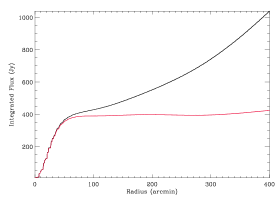
Figure 1: Integrated flux at 23 GHz as a function of the angular distance to the Crab nebula center before (black) and after (red) background subtraction.

In this paper we are mainly interested in the microwave and millimetre regime for which the best currently available data are the WMAP Page et al. (2007) and Archeops Desert et al. (2008) data. To avoid any bias on our analysis by a difference of treatment of these two data sets we have decided to re-estimate the Crab nebula unpolarised emission from 23 to 545 GHz using the publicly available WMAP Page et al. (2007); Hinshaw et al. (2009) and Archeops Macías-Pérez et al. (2007) intensity maps. Furthermore, to make the full data set as homogeneous as possible, the total intensity flux for each frequency was estimated using standard radial photometry techniques to mimic the flux integration performed for the high resolution data sets. Notice that we integrate far from the radio extension of the Crab nebula, $\sim$ 5 arcminutes radius, to recover the Crab nebula flux diluted over the entire beam pattern, Therefore, a key issue for this analysis is the subtraction of the background galactic emission which is mainly due to synchrotron and free–free emissions at low frequencies and dust at high frequencies. As the WMAP and Archeops maps are available on Healpix format we have develop our own radial photometry software for this pixelization scheme.

The results of this analysis are presented on table 1. For Archeops we obtain similar values than those in Desert et al. (2008) with slightly different error bars. However, for WMAP we obtain values 8 % larger than those in Page et al. (2007). Most probably the difference comes from the way the background subtraction is performed and the fact the WMAP team computed the intensity and polarisation simultaneously. It is important to stress that the difference with respect to the WMAP team is within the 1–$\sigma$ error bars at high frequency and goes up to 3–$\sigma$ at 23 GHz. To illustrate the problem of background subraction we show on figure 1 the radial profile centered at the Crab nebula position before (black) and after (red) background subtraction at 23 GHz. For this paper we use our own estimation of the Crab nebula flux in intensity but we have noticed that the final conclusions are not changed significantly by the choice of data set.

3 SED of the Crab Nebula

We present in this section a coherent analysis of the Crab SED in the range 1 to 10⁶ GHz based on a compendium of observations shown in Table 1. Notice that to be able to directly compare to the Archeops and WMAP data, we have chosen only those data sets for which integrated fluxes over the full extension of the Crab Nebula are available.

$\nu$ (GHz)	$\rm S_{\nu}$ (Jy)	$\rm\Delta S_{\nu}$ (Jy)	Central Epoch	Reference
1.117	990.0	59.4	1969.9	Vinogradova et al. (1971)
1.304	980.0	58.8	1969.9	Vinogradova et al. (1971)
1.4	930.0	46.5	1963	Kellermann et al. (1969)
1.765	940.0	56.4	1969.9	Vinogradova et al. (1971)
2.0	840.0	50.4	1969.3	Dmitrenko et al. (1970)
2.29	810.0	48.6	1969.3	Dmitrenko et al. (1970)
2.74	795.0	47.7	1969.3	Dmitrenko et al. (1970)
3.15	700.0	24.5	1964.4	Medd (1972)
3.38	718.0	43.1	1969.3	Dmitrenko et al. (1970)
3.96	646.0	38.8	1969.3	Dmitrenko et al. (1970)
4.08	687.0	20.6	1964.8	Penzias & Wilson (1965)
5.0	680	34	1963	Kellermann et al. (1969)
6.66	577.2	20.2	1965.	Medd (1972)
8.25	563.0	22.5	1965.9	Allen & Barrett (1967)
13.49	524.0	19.9	1969.9	Medd (1972)
15.5	461	24	1965.9	Allen & Barrett (1967)
16.0	447.0	15.6	1970.6	Wrixon et al. (1972)
22.285	397	16.0	1973.1	Janssen et al. (1974)
22.5	395	7	2003	This paper
31.41	387	72	1966.7	Hobbs et al. (1968)
32.8	340	5	2003	This paper
34.9	340	68	1967.3	Kalaghan & Wulfsberg (1967)
40.4	323	8.0	2003	This paper
60.2	294	10.0	2003	This paper
92.9	285	16.0	2003	This paper
111,1	290	35	1973.5	Zabolotnyi et al. (1976)
143	231	32	2002	This paper
217	182	38	2002	This paper
230	260	52	2000	Bandiera et al. (2002)
250	204	32	1985.3	Mezger et al. (1986)
300	194.0	19.4	1983	Chini et al. (1984)
300	131	42	1978.75	Wright et al. (1979)
300	300	80	1976.0	Werner et al. (1977)
347	190	19	1999.8	Green et al. (2004)
353	186	34	2002	This paper
545	237	68	2002	This paper
750	158	63	1978.75	Wright et al. (1979)
1000	135	41	1978.75	Wright et al. (1979)
3000	184	13	1983.5	Strom & Greidanus (1992)
5000	210	8	1983.5	Strom & Greidanus (1992)
$\rm 12\times 10^{3}$	67	4	1983.5	Strom & Greidanus (1992)
$\rm 25\times 10^{3}$	37	1	1983.5	Strom & Greidanus (1992)
$3.246\times 10^{5}$	6.57	0.66	1989	Veron-Cetty & Woltjer (1993)
$4.651\times 10^{5}$	4.78	0.48	1989	Veron-Cetty & Woltjer (1993)
$5.593\times 10^{5}$	4.23	0.42	1989	Veron-Cetty & Woltjer (1993)
$7.878\times 10^{5}$	3.22	0.32	1989	Veron-Cetty & Woltjer (1993)

Table 1: Compendium of Crab Nebula observations from 1 to $\rm 10^{6}\ GHz$. Fluxes ($\rm S_{\nu}$) are presented in Jy. For Veron-Cetty & Woltjer 1993 and Chini et al. 1984 a conservative 10% error has been chosen to account for extrapolation errors. The central epoch of observation is also indicated. This is used for the evaluation of the fading effect of the low frequency synchrotron component, up to 100 GHz. Data values labeled This paper for Archeops and WMAP are revaluated using the method described in Section 2.

3.1 Low-frequency synchrotron emission

An accurate determination of the low-frequency synchrotron component is necessary to assess the synchrotron contribution at mm frequencies. Any inter-comparison of low-frequency radio observations of the Crab nebula must take into account its well-known secular decrease. In particular Aller & Reynolds (1985) have estimated a secular decrease in the flux density at a rate $\alpha=(-0.167\pm 0.015)\ \%yr^{-1}$ from observations at $\rm 8\ GHz$ over the period 1968 to 1984. This result is in good agreement with other studies at lower frequencies: for example $\alpha=(-0.18\pm 0.1)\ \%yr^{-1}$ over the period 1977 to 2000 at $\rm 927\ MHz$ by Vinyajkin (2005).

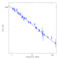
Figure 2: SED of the Crab Nebula from 1 to 100 GHz. Data samples are represented together. with he best-fit power law model to the data (see text for details).

Figure 3: High frequency SED of the Crab Nebula. Data samples are represented together with the. best-fit power law model to the data (see text for details).

All these measurements are in fair agreement with theoretical evaluations of the evolution of pulsar driven supernova remnants by Reynolds & Chevalier (1984) which predicts $\rm\alpha$ ranging from $-0.16\%$ to $-0.4\%yr^{-1}$.
For this paper the value $\alpha=-0.167\ \%yr^{-1}$ is chosen for the fading of the Crab Nebula and all data are converted to a common observation date, 01/01/2003. In figure 2 we trace the flux of the Crab Nebula as a function of frequency for the fading corrected low-frequency data in table 1 ranging from 1 to 143 GHz.

We observe a large decrease of flux with increasing frequency which can be represented by a power law of the form $\rm A_{1}\big{(}\frac{\nu}{1\mathrm{GHz}}\big{)}^{\beta_{1}}$. By $\chi^{2}$ minimization, we obtain for the low-frequency data up to 100 GHz

$$\beta_{1}=-0.296\pm 0.006\;\textnormal{and}\;A_{1}=(973\pm 19)\ Jy$$

with $\rm\chi^{2}/N_{dof}=1.03$ and this model is shown as a solid line on Fig 2. This result is in agreement with the ”canonical” value $\beta\simeq-0.299\pm 0.009$ from Baars et al. (1977) at the 1-$\sigma$ level.

3.2 High frequency synchrotron and dust emission

Figure 4: Residual to the standard model of the Crab nebula emission assuming a synchrotron and a dust component, in the range 10 to 2000 GHz (see text for details). Notice that the millimetric data were not used in the fit. We show the full data set in the region of interest.

The Crab synchrotron emission described above evolves at higher frequencies, around $10^{4}$ GHz, towards a much harder SED with a spectral index of $\sim-0.73$ (see for example Veron-Cetty & Woltjer (1993)). To accurately estimate the synchrotron emission properties at high frequency we have fitted the data from $10^{4}$ to $\rm 10^{6}\ GHz$ presented in table 1 to a power law of the form $\rm A_{2}\nu^{\beta_{2}}$. By $\chi^{2}$ minimization, we found the data to be well fitted, $\rm\chi^{2}/N_{dof}=0.155$, by a power law of parameters

$$\rm\beta_{2}=(-0.698\pm 0.018)\;\textnormal{and}\;A_{2}=(43.5\pm 8.8)\times 10^{3}\,Jy$$

Figure 3 represents the high-frequency data and the best-fit power law model is overplotted.

Finally, the infrared satellite observatory IRAS has revealed significant excess emission above this synchrotron contribution around 50 $\rm\mu m$ Marsden et al. (1984). As shown by Strom & Greidanus (1992) this can be explained, after careful removing of the synchrotron component, by a single dust component described by a modified black body of emissivity $\beta=2$ at T$\rm=46\pm 3\ K$, requiring a dust mass of $\rm 0.02\ M_{\odot}$.

3.3 Millimetric excess

To evaluate a possible millimetric excess of flux in the range 100 to 1000 GHz we assume the above canonical modeling of the Crab nebula SED: a synchrotron component with a spectral index break at high frequency and a dust component at infrared wavelengths. We can thus reconstruct the Crab nebula emission at the millimetric frequencies and compare it to the data in table 1. Fig 4 shows the residuals to the canonical model from 10 to $2\times 10^{4}$ GHz. We observe that there is no significant excess of power in the millimetric regime from 100 to 1000 GHz except for the 545 GHz Archeops data sample which presents only a 1.5 sigma excess. Indeed, the $\chi^{2}/N_{dof}$ for the null hypothesis is $0.69$.

4 Refined modeling

In the previous section we have proved that the millimetric data in table 1, from 100 to 1000 GHz, are compatible with the canonical model assuming single synchrotron and dust components. However, it is interesting to check if an extra component may improve significantly the fit to the data. Following Bandiera et al. (2002) we consider either an extra low-temperature dust emission or an extra synchrotron component. Thus, the three component model is defined as follows

1. Canonical synchrotron that is described by four parameters: spectral index and amplitude for the low and high frequency emission. At high frequency we consider both the amplitude and the spectral index fixed and set them to the values obtained in Sect. 3.2. At low frequency we fix the spectral index to the value obtained in Sect. 3.1 and the amplitude, $A_{S}$, is fitted. We also assume a constant fading of $\alpha=-0.167\ \%yr^{-1}$ as before.

2. Canonical dust (following Strom & Greidanus (1992)) described by a modified black body with three free parameters, $A_{D}$, $T_{D}$ and $\beta_{D}$ that represent the amplitude, temperature and spectral index respectively.

3. One of the extra components as described below.

4.1 Extra low-temperature dust emission

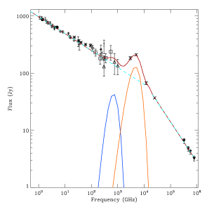
Figure 5: Refined modelling of the SED of the Crab nebula in the frequency range from 1 to 10⁶ GHz assuming an extra dust component at low-temperature. Left panel: We represent the data from table 1 (black), the best-fit model to the data (red) and the synchrotron (light blue), the main dust (orange) and the extra dust (dark blue) components associated to it. Right panel: residuals in the millimetric regime for the top panel models.

$\chi^{2}/N_{dof}$	$A_{s}\ \mathrm{(Jy)}$	$A_{D}\ \mathrm{(Jy)}$	$T_{D}\ \mathrm{(K)}$	$\beta_{D}$	$A_{LTD}\ \mathrm{(Jy)}$	$T_{LTD}\ \mathrm{(K)}$	$\beta_{LTD}$	LTD %	$\chi^{2}_{mm}/N_{dof}$
0.73	$971\pm 9$	$128\pm 8$	$45.9\pm 1.2$	$1.93\pm 0.50$	$32\pm 24$	$5\pm 23$	$3.6\pm 2.4$	$26\pm 20$	0.88

Table 2: Best-fit model parameters and errors for the extra dust component model. $\chi^{2}/N_{dof}$ for the full data set and on the millimetric regime from 100 to 1000 GHz. LTD % stands for the percentage of flux at 545 GHz due to the extra dust component with respect to the total flux.

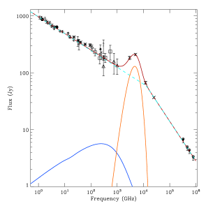
Figure 6: Refined modelling of the SED of the Crab nebula in the frequency range from 1 to 10⁶ GHz assuming an extra synchrotron component. Left panel: We represent the data from table 1 (black), the best-fit model to the data (red) and the main synchrotron (light blue), the extra synchrotron (dark blue) and the dust components (orange) associated to it. Right panel: residuals in the millimetric regime for the top panel models.

$\chi^{2}/N_{dof}$	$A_{s}\ \mathrm{(Jy)}$	$A_{D}\ \mathrm{(Jy)}$	$T_{D}\ \mathrm{(K)}$	$\beta_{D}$	$A_{LECS}\ \mathrm{(Jy)}$	$\nu_{c}\ \mathrm{(GHz)}$	$p$	LECS %	$\chi^{2}_{mm}/N_{dof}$
$0.76$	$965\pm 14$	$129\pm 9$	$46.0\pm 1.0$	$1.89\pm 0.4$	$5\pm 6$	$470\pm 317$	$3\pm 12$	$3\pm 3$	0.93

Table 3: Best-fit model parameters and errors for the extra syncrotron component model. $\chi^{2}/N_{dof}$ for the full data set and on the millimetric regime from 100 to 1000 GHz. LECS % stands for the percentage of flux at 545 GHz due to the extra synchrotron component with respect to the total flux.

In Sect. 3.3 we concluded that at $\rm 545\ GHz$ the difference between the standard model and the data is at its maximum. In the case of an extra dust component this implies very low temperature dust (LTD) in the range from 4 to 10 K. To model this component we assume a modified black body spectrum with three free parameters $A_{LTD}$, $T_{LTD}$ and $\beta_{LTD}$ that represent the amplitude, temperature and spectral index respectively. The best-fit model to the data is found by $\chi^{2}$ minimization on the full frequency range from 1 to 10⁶ GHz.

Figure 5 presents on the left panel the observational data (black) and the global best-fit model to the data (in red). The canonical synchrotron component is shown on light blue and the canonical dust in orange. The extra low temperature dust component is represented in blue. The right panel presents the residuals to the best fit-model in the frequency range of interest. The parameters and error bars for the best-fit model to the data and the percentage of flux at 545 GHz associated to the extra component with respect to the total flux are given in table 2. We also present the $\chi^{2}/N_{dof}$ values for the global fit in the frequency range from 1 to 10⁶ GHz and on the millimetric range from 100 to 1000 GHz.

We obtain a good global fit to the data as shown by the $\chi^{2}/N_{dof}$ value. The best-fit parameters obtained for the canonical synchrotron and dust components are in good agreement with those presented in Sect. 3. Comparing with Strom & Greidanus (1992), we found the same dust temperature, $46\pm 1$ K, with an error bar improved by a factor of three, as we carefully account for the canonical synchrotron spectrum. The amplitude of the extra component is compatible with zero and therefore we conclude that there are no evidence for an extra component in the form of low–temperature dust. Furthermore, we observe that on the one hand the data require extremely low temperatures of $5$ K with rather large error bars, therefore dust masses of $\rm\sim 230\ M_{\odot}$, making the model rather unrealistic. On the other hand, the improvement of the $\chi^{2}/N_{dof}$ in the millimetric region between 100 and 1000 GHz is not significant to justify the addition of the three extra parameters required by the low-temperature dust component. This is also clear on the right panel of figure 5 where we represent the residuals to the best-fit model to the data on the millimetric regime.

4.2 Extra synchrotron component

For the extra synchrotron component we consider, as in Bandiera et al. (2002), that the distribution of energy of the relativistic electrons responsible for the emission is well represented by a power law with spectral index in the range 1 to 3 and present a low-energy cutoff. To account for an excess of flux in the millimeter regime, the critical frequency corresponding to the lowest energy electrons must be somewhere in the range 200 to 600 GHz. In total the low-energy cutoff synchrotron (LECS) model has three parameters, $p$ the spectral index of the electron energy distribution, $\nu_{c}$ the low-energy cutoff critical frequency and $A_{LECS}$, a normalization coefficient. The best-fit to the data is found by $\chi^{2}$ minimization.

The parameters and error bars of the best-fit to the data for the three data sets as well as the percentage of flux due to the extra component with respect to the total flux at 545 GHz are given on table 3. We also present $\chi^{2}/N_{dof}$ values for the best-fit to the data on the full data set from 1 to 10⁶ GHz and on the millimetric regime from 100 to 1000 GHz.The left panel of figure 6 presents the data in black and the global best-fit model to the data is represented in red. The canonical synchrotron component is shown on light blue and the canonical dust in orange. The extra low-energy cutoff synchrotron component is represented in blue.

As above, we obtain a good global fit to the data as shown by the $\chi^{2}/N_{dof}$ value. The best-fit parameters obtained for the canonical synchrotron and dust components are in good agreement with those presented in Sect. 3 and on Strom & Greidanus (1992). The amplitude of the extra synchrotron component is compatible with zero as well as the value of the spectral index of the electron energy distribution. We therefore conclude that there is no evidence of an extra component in the form of low-energy cutoff synchrotron. In addition, we observe that the $\chi^{2}/N_{dof}$ in the millimetric region from 100 to 1000 GHz is worse than the one obtained in Sect 3.3 assuming the canonical model only. The right panel of figure 6 represents the residuals to the best-fit model to the data on the millimetric regime. From this we conclude that the fit to the data in this frequency regime is not improved by adding an extra synchrotron component.

We have also performed the analysis of the data set considering the $p$ and $\nu_{c}$ parameters fixed and set to the values quoted by Bandiera et al. (2002). The analysis shows that the amplitude of the extra synchrotron component is compatible with zero and therefore we conclude that the data show no evidence of an extra synchrotron component.

5 Implications for the Planck satellite polarisation calibration

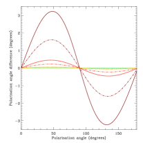
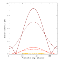
Figure 7: Errors induced in the degree and angle of polarisation by an extra low–temperature dust component. Left plot: relative error on the degree of polarisation on the case of an unpolarised extra component as a function of the frequency of the polarised Planck channels. Middle plot and right plot: relative error on the degree of polarisation and polarisation angle error on the case of an extra polarised component as a function of the polarisation angle of this component. The dashed and solid lines correspond to an extra component with a degree of polarisation of 5 % and 10 % respectively. From blue to red we represent the values for the different polarised Planck channels from 30 to 353 GHz.

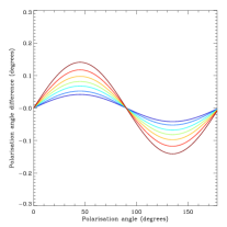
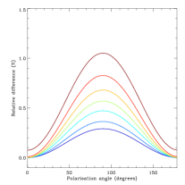
Figure 8: Errors induced in the degree and angle of polarisation by an extra low–energy cutoff synchrotron component. Left plot: relative error on the degree of polarisation on the case of an unpolarised extra component as a function of the frequency of the polarised Planck channels. Middle plot and right plot: relative error on the degree of polarisation and polarisation angle error on the case of an extra polarised component as a function of the polarisation angle of this component. From blue to red we represent the values for the different polarised Planck channels from 30 to 353 GHz.

From the previous section, we conclude that the intensity emission of the Crab nebula at millimetre and submillimetre wavelengths is dominated by the well known synchrotron radiation observed at radio wavelengths. The data show no evidence of an extra synchrotron component and evidence for an extra dust component is not significant. Therefore, we can postulate that the Crab nebula emission at millimetre and submillimetre wavelengths is produced by the same relativistic electrons that the ones producing the radio emission. Then it is reasonable to guess that Crab nebula presents the same polarisation properties at radio and millimetre wavelengths. These conclusions are also supported by the Crab polarised emission observed from 23 to 94 GHz by the WMAP satellite Page et al. (2007) when compared to the 363 GHz SCUBA measurements Greaves et al. (2003) and the Flett & Murray (1991) 273 GHz data. From these, it makes sense to use the low–frequency observations of the Crab nebula to cross-check and eventually update the knowledge of the polarisation characteristics of the high–frequency instruments as proposed by the Planck collaboration. As a summary and using the results from Page et al. (2007); Greaves et al. (2003); Flett & Murray (1991) we expect the Crab nebula emission at the Planck frequencies to be polarised with a degree of polarisation of 8 to 9 % and a polarisation angle of 150^∘ in equatorial coordinates Aumont (2009). Then, at 30 GHz and 353 GHz we expect the total intensity to be $351\pm 7$ and $173\pm 5$ Jy and the polarised intensity about 28 and 15 Jy, respectively.

However, we can estimate upper limits on the errors induced on the determination of the degree of polarisation and polarisation angle of the Crab nebula emission at the Planck observation frequencies by the presence of an extra component. For this we use the results obtained on the previous section and we assume two different cases: polarised and unpolarised extra component. Figure 7 shows 1-$\sigma$ upper limits on the case of a low–temperature dust extra component. For the left plot we assume an unpolarised extra component and we present the error on the determination of the degree of polarisation as a function of the observation frequency. This error is below 1 % for the Planck CMB channels from 70 to 217 GHz and rise up to 8% at 353 GHz. The middle and right plot assume a polarised extra component and show the error on the polarisation angle and degree of polarisation, respectively, as a function of the polarisation angle of the extra component with respect to the main synchrotron component. From blue to red we show the errors from 30 to 353 GHz. The dotted-dashed and solid curve assume a degree of polarisation of 5 and 10 % for the extra component. As before the error on the degree of polarisation is below 1 % at the CMB channels and from 12 to 18 % at 353 GHz. For the polarisation angle the error is below 0.2^∘ for the CMB channels and at maximum of 3^∘ at 353 GHz. Notice that the increase in the errors at 353 GHz is mainly due to the large value and large error bars of the Archeops data at 545 GHz and we do not think it is significant. Figure 8 shows the errors induced by an extra low-energy cutoff synchrotron component either unpolarised or polarised with a degree of polarisation equivalent to the one expected for the canonical synchrotron component. In this case the errors are much lower being well below 1 % and 0.2^∘ for the degree and angle of polarisation, respectively, at all polarised Planck frequencies.

6 Summary and conclusions

Within the framework of the polarisation calibration of the Planck satellite emission we present in this paper a global analysis of the SED of the Crab Nebula in the frequency range from 1 to 10⁶ GHz. For this purpose we have used new data from the WMAP satellite Page et al. (2007) and from the Archeops balloon experiment Desert et al. (2008) in addition to data currently available. We focus on the centimetric and millimetric regime as Planck observes the sky from 30 to 857 GHz.

We have first shown that the data are compatible with the canonical model of Crab nebula emission which assumes a synchrotron component at low and high frequencies, plus a dust component at the micrometre wavelengths. To check if an extra component may improve significantly the fit to the data, we consider either an extra low-temperature dust emission or an extra low-energy cutoff synchrotron component, as in Bandiera et al. (2002). In both cases, we conclude that the current data present no evidence of an extra component. Therefore, the un-polarised millimetre flux of the Crab nebula is well represented by the following synchrotron power–law model

$$F_{\nu}=973\ \pm\ 19\,\mathrm{Jy}\ {\big{(}\frac{\nu}{\mathrm{1\ GHz}}\big{)}}^{(-0.296\ \pm\ 0.006)}\ \exp{(\alpha(\mathrm{T}_{\mathrm{obs}}-2003))}$$ (1)

where $\alpha=-1.67\times 10^{-3}\ \mathrm{yr}^{-1}$ is the synchrotron fading and $\nu$ and $\mathrm{T}_{\mathrm{obs}}$ are the frequency and the date of observation in years A.C., respectively.

From above, we can conclude that the millimetre emission of the Crab nebula has the same physical origin than the radio synchrotron emission and therefore it is expected to be polarised with the same degree of polarisation and the same orientation. From the current data set we estimate that the errors on the reconstruction of the degree and angle of polarisation on the Planck cosmological channels induced by an extra component will be well below 1 %. This result strongly supports the choice by the Planck collaboration of the Crab nebula emission for performing polarisation cross-checks in the range 30 to 353 GHz Aumont (2009).

References

- Aller & Reynolds (1985) Aller H. D. & Reynolds S. P., 1985, ApJ, 293, L73
- Allen & Barrett (1967) Allen R. J. & Barrett A. H., 1967, ApJ, 149, 1
- Aumont (2009) Aumont, J., 2009, A&A, submitted
- Baars & Hartsuijker (1972) Baars J. W. M., Hartsuijker A. P. , 1972, A&A, 17, 172
- Baars et al. (1977) Baars J. W. M. et al., 1977, A&A, 61, 99
- Bandiera et al. (2002) Bandiera R. et al., 2002, A&A, 386, 1044
- Becklin & Kleinmann (1968) Becklin E. E. & Kleinmann D. E., 1968, ApJ, 152, L25
- Chini et al. (1984) Chini R. et al., 1984, A&A, 137, 117-127
- Dmitrenko et al. (1970) Dmitrenko T. et al., 1970, Radiofizika, Vol. 13, No. 6, 823-829
- Desert et al. (2008) Desert F.-X., Macías-Pérez J. F. , Mayet F. et al., 2008, A&A, 481, 411-421
- Flett & Murray (1991) Flett, A. M. & Murray, A.G. 1991, MNRAS, 249, 4P
- Grasdalen (1979) Grasdalen G. L., 1979, PACS, 91, 436
- Greaves et al. (2003) Greaves, J. S., Holland, W. S., Jenness, T., et al. 2003, MNRAS, 340, 353
- Hinshaw et al. (2009) Hinshaw, B., et al., 2009, ApJ, 180, 225-245
- Green et al. (2004) Green D.A., Tuffs R.J. & Popescu C.C., 2004, MNRAS, 355, 1315-1326
- Hobbs et al. (1968) Hobbs R. W., Corbett H. H., Santini N. J., 1968, ApJ, 152, 43
- Janssen et al. (1974) Janssen M. A., Golden L. M. and Welch W. J., 1974, A&A, 33, 373-377
- Kalaghan & Wulfsberg (1967) Kalaghan P. M. and Wulfsberg K. N., 1967, Astronomical J. , 72, 1051
- Kellermann et al. (1969) Kellermann K. I., Pauliny-Toth I. I. K., Williams P. J. S., 1969, ApJ, 157, 1
- Kovalenko et al. (1994) Kovalenko A. V., Pynzar’ A. V., Udal’tsov V. A., 1994, Astronomy Reports, 38, 78-94
- Macías-Pérez et al. (2007) Macías-Pérez J. F. et al., 2007, A&A, 467, 1313
- Marsden et al. (1984) Marsden P. L. et al., 1984, ApJ, 278, L29
- Medd (1972) Medd W. J., 1972, ApJ, 171, 41
- Mezger et al. (1986) Mezger P. G. et al., 1986, A&A, 167, 145
- Page et al. (2007) Page, L. et al., 2007, ApJ, 170, 335
- Penzias & Wilson (1965) Penzias A. A. and Wilson R. W., 1965, ApJ, 142, 1149
- Reynolds & Chevalier (1984) Reynolds S. P., Chevalier R. A., 1984, ApJ, 278, 630
- Strom & Greidanus (1992) Strom R. G. & Greidanus H., 1992, Nature, 358, 654
- Veron-Cetty & Woltjer (1993) Véron-Cetty M. P. & Woltjer L., 1993, A&A, 270, 370
- Vinogradova et al. (1971) Vinogradova L. V. et al., 1971, Radiofizika, Vol. 14, No. 1, 157-159
- Vinyajkin (2005) Vinyajkin E. N., 2005, astro-ph/0502033
- Werner et al. (1977) Werner M. W. et al., 1977, PACS, 89, 127
- Wright et al. (1979) Wright E. L. et al., 1979, Nature, 279,703
- Wrixon et al. (1972) Wrixon G. T. et al., 1972, ApJ, 174, 399
- Zabolotnyi et al. (1976) Zabolotnyi V. F., Kostenko V. I., Slysh V. I. 1976, Soviet Astronomy, 19, 405