Maximal Quantum Violation of the CGLMP Inequality on Its Both Sides

Abstract

Abstract

We investigate the maximal violations for both sides of the $d$-dimensional CGLMP inequality by using the Bell operator method. It turns out that the maximal violations have a decelerating increase as the dimension increases and tend to a finite value at infinity. The numerical values are given out up to $d=10^{6}$ for positively maximal violations and $d=2\times 10^{5}$ for negatively maximal violations. Counterintuitively, the negatively maximal violations tend to be a little stronger than the positively maximal violations. Further we show the states corresponding to these maximal violations and compare them with the maximally entangled states by utilizing entangled degree defined by von Neumann entropy. It shows that their entangled degree tends to some nonmaximal value as the dimension increases.

Bell inequality 1964Bell , arising from the Einstein-Podolsky-Rosen (EPR) paradox 1935Einstein , has developed into an effective criterion between the classical and quantum theory. The famous Clauser-Horne-Shimony-Holt (CHSH) inequality CHSH for two entangled spin-1/2 particles has always provided an excellent test-bed for experimental verification of quantum mechanics against the predictions of local realism. In 2002, two research teams independently developed Bell inequalities for high-dimensional systems: the first one is a Clauser-Horne type (probability) inequality for two qutrits 2002Kaszlikowski ; 2002Chen ; the second one is a CHSH type inequality for two qu$d$its ($d$ is an arbitrarily high dimension), now known as the Collins-Gisin-Linden-Masser- Popoescu (CGLMP) inequality 2002Collins . The tightness of the CGLMP inequality was demonstrated in Ref. 2002Lluis . Such an inequality is later modified into more compact forms 2004Fu ; 2005Chen and its numerical violations for high-dimensional situations have also been investigated in 2006Chen ; 2008Gill .

The CGLMP inequality for two $d$-dimensional systems is constrained by two classical bounds at its two sides, one being positive and the other negative 2005Chen . Both two classical bounds can be violated by quantum behaviors. Such a property provides us the chance to inspect the quantum nonlocality in the high-dimensional cases. In principle, the maximally violating values of the inequality can be achieved by searching all possible measurements on all kinds of entangled states including mixed states. However, the complexity of numerical simulation will increases in power as the dimension increases, mainly because the number of variable parameters during the searching process is proportional to $d^{2}+d$ (for pure states). In Ref. 2006Chen , Chen et al. have investigated the maximal quantum violation of the CGLMP inequality at its positive side by using the Bell operator method. Such a method has a merit that it transforms the maximal violation problem into a pure mathematical calculation of solving the maximal and minimal eigenvalues of a matrix. By doing this, it needs a prerequisite that a set of phase rules for fixing the measurement projectors must be known so as to explicitly give out the matrix elements. In general, the determination of these rules needs a large quantity of numerical simulations. As it is, the rule for obtaining the positively maximal violation of the CGLMP inequality has been known before 2006Chen ; 2002Collins , but the one for the negatively maximal violation is still unknown. Physically, it is necessary for us to examine whether the negative violation is larger than the positive side, since a stronger quantum nonlocality may be indicated while the positive violation would be enough if that is not the case.

In this paper, we first simplify the Bell operator method appeared in 2006Chen and then give out, respectively, the phase rules for obtaining the positively and negatively maximal violations of the CGLMP inequality. After that, the matrix elements of Bell operator are derived. Numerical results about maximal quantum violations are achieved by solving the maximal and minimal eigenvalues of the Bell operator. At last, the strength of quantum nonlocality is compared between the positive and negative violations, and their corresponding states are also discussed.

The CGLMP inequality as an extended version of the Bell-CHSH inequality for $d$-dimensional Hilbert space has the form 2004Fu

$$I_{d}=Q_{11}+Q_{12}-Q_{21}+Q_{22},$$ (1)

where $Q_{ij}$ are the Bell-type correlation functions defined by probabilities in the way

$$Q_{ij}=\frac{1}{S}\sum_{m=0}^{d-1}\sum_{n=0}^{d-1}f^{ij}(m,n)P(A_{i}=m,B_{j}=n),$$ (2)

with the spin $S=(d-1)/2$ and eigenvalues of the correlation function, $f^{ij}(m,n)=S-M(\varepsilon(i-j)(m+n),d)$ [$\varepsilon(x)=1$ for $x\geq 0$ and $-1$ for $x<0$; $M(x,d)=x\;{\rm mod}\;d$.]. In classical theory, the Eq. (1) has two bounds 2005Chen as

$$-2(\delta_{2d}+(1-\delta_{2d})\frac{d+1}{d-1})\leq I_{d}\leq 2,$$ (3)

which can be violated in quantum theory. Following 2002Kaszlikowski ; 2002Collins ; 2002Acin ; 2001Durt ; 2000Kaszlikowski ; 2006Chen , we use the unitary transformation setting of unbiased multiport beam splitters (UMBS) 1997Zukowski ; 2000Kaszlikowski instead of a complete $d$-dimensional unitary transformation to define projectors [see Eq. (5)]. Unbiased $d$-port beam splitter (see Fig. 1) is a device with the following property: if a photon enters any of the $d$ single input ports, its chances of exit are equally split among the $d$ output ports. In fact one can always build the device with the distinguishing trait that the elements of its unitary transition matrix $T$ are solely powers of the root of unity $\gamma=\exp(i2\pi/d)$, namely, $T_{kl}=\frac{1}{\sqrt{d}}\gamma^{kl}$. In front of $i$th input port of the device a phase shifter is placed to change the phase of the incoming photon by $\phi(i)$. These $d$ phase shifts, denoted for convenience as a “vector” of phase shifts $\hat{\phi}=(\phi(0),\phi(1),\cdots,\phi(d-1))$, are macroscopic local parameters that can be changed by the observer. Therefore, unbiased $d$-port beam splitter together with the $d$ phase shifters perform the unitary transformation $U(\hat{\phi})$ with the entries $U_{kl}=T_{kl}\exp[i\phi(l)]$. The diagram of such unitary operation has been displayed in the Fig. 1.

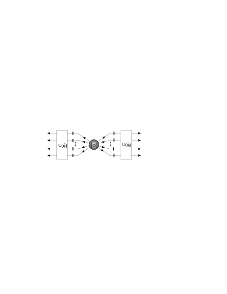
Figure 1: The diagram of unbiased multiport beam splitter. In front of the $i$th input port of the device a phase shifter is placed to change the phase of the incoming photon by $\phi(i)$. The whole action can be described by unitary operator $U(\hat{\phi}_{a})$ and $U(\hat{\varphi}_{b})$.

An arbitrary entangled state of two qudits after Schmidt decomposition reads

$$|\Phi\rangle=\sum_{i=0}^{d-1}\alpha_{i}|ii\rangle,$$ (4)

with Schmidt coefficients $\{\alpha_{i}\}$ being real and satisfying normalization condition $\sum_{i}|\alpha_{i}|^{2}=1$ 2000Nielsen . One can see that if we take $\alpha_{i}=1/\sqrt{d}$ for all $i$ it is just the maximally entangled state. The quantum prediction of the joint probability $P(A_{a}=k,B_{b}=l)$ when $A_{a}$ and $B_{b}$ are measured in the initial state $|\Phi\rangle$ is given by

$$P(A_{a}=k,B_{b}=l) = \langle\Phi|\hat{P}(A_{a}=k)\otimes\hat{P}(B_{b}=l)|\Phi\rangle$$ (5)

$$= {\rm Tr}\left[(U(\hat{\phi}_{a})^{\dagger}\otimes U(\hat{\varphi}_{b})^{\dagger})\;\hat{\Pi}_{k}\otimes\hat{\Pi}_{l}\;(U(\hat{\phi}_{a})\otimes U(\hat{\varphi}_{b}))\;|\Phi\rangle\langle\Phi|\right]$$

$$= \frac{1}{d^{2}}\sum_{j,m=0}^{d-1}\alpha_{j}\alpha_{m}e^{i[\frac{2\pi}{d}(j-m)(k-l)+\phi_{a}(j)-\phi_{a}(m)+\varphi_{b}(j)-\varphi_{b}(m)]}$$

$$= \frac{1}{d^{2}}\sum_{j,m=0}^{d-1}\alpha_{j}\alpha_{m}\cos\left[\frac{2\pi}{d}(j-m)(k-l)+\phi_{a}(j)-\phi_{a}(m)+\varphi_{b}(j)-\varphi_{b}(m)\right],$$

where $\hat{\Pi}_{k}=|k\rangle\langle k|$, $\hat{\Pi}_{l}=|l\rangle\langle l|$ are the projectors for observers $A$ and $B$ not including UMBS transformation, respectively. Substituting Eq. (5) into the high-dimensional Bell inequality (1), one gets the Bell expression for the state $|\Phi\rangle$:

$$I_{d}(|\Phi\rangle) = \frac{1}{d}\sum_{j,m=0}^{d-1}\alpha_{j}\alpha_{m}\left[e^{i[\phi_{1}(j)-\phi_{1}(m)+\varphi_{1}(j)-\varphi_{1}(m)]}\sum_{k=0}^{d-1}\left(1-\frac{2k}{d-1}\right)e^{i\frac{2\pi}{d}k(j-m)}\right.$$ (6)

$$+e^{i[\phi_{1}(j)-\phi_{1}(m)+\varphi_{2}(j)-\varphi_{2}(m)]}\sum_{k=0}^{d-1}\left(1-\frac{2k}{d-1}\right)e^{-i\frac{2\pi}{d}k(j-m)}$$

$$-e^{i[\phi_{2}(j)-\phi_{2}(m)+\varphi_{1}(j)-\varphi_{1}(m)]}\sum_{k=0}^{d-1}\left(1-\frac{2k}{d-1}\right)e^{i\frac{2\pi}{d}k(j-m)}$$

$$\left.+e^{i[\phi_{2}(j)-\phi_{2}(m)+\varphi_{2}(j)-\varphi_{2}(m)]}\sum_{k=0}^{d-1}\left(1-\frac{2k}{d-1}\right)e^{i\frac{2\pi}{d}k(j-m)}\right].$$

By using the summation formula

$$\sum_{k=0}^{d-1}\left(1-\frac{2k}{d-1}\right)e^{i\frac{2\pi}{d}k(j-m)}=\frac{2d}{(d-1)[1-e^{i\frac{2\pi}{d}(j-m)}]},\quad(j\neq m)$$

we can reduce Eq. (6) to a real-valued expression, i.e.,

$$I_{d}(|\Phi\rangle) = \frac{1}{d-1}\sum_{j\neq m}^{d-1}\alpha_{j}\alpha_{m}\frac{1}{\sin\left[\frac{\pi}{d}(j-m)\right]}\bigg{\{}-\sin\left[\phi_{1}(j)-\phi_{1}(m)+\varphi_{1}(j)-\varphi_{1}(m)-\frac{\pi}{d}(j-m)\right]$$ (7)

$$+\sin\left[\phi_{1}(j)-\phi_{1}(m)+\varphi_{2}(j)-\varphi_{2}(m)+\frac{\pi}{d}(j-m)\right]$$

$$+\sin\left[\phi_{2}(j)-\phi_{2}(m)+\varphi_{1}(j)-\varphi_{1}(m)-\frac{\pi}{d}(j-m)\right]$$

$$-\sin\left[\phi_{2}(j)-\phi_{2}(m)+\varphi_{2}(j)-\varphi_{2}(m)-\frac{\pi}{d}(j-m)\right]\bigg{\}}.$$

From Eq. (7), we can see that $I_{d}$ depends on the state coefficients $\{\alpha_{i}\}$ and phase shifts $\{\phi_{1,2}(j),\varphi_{1,2}(m)\}$. For the positively maximal values of $I_{d}$, there have been several investigations: when $|\Phi\rangle$ is restricted in maximally entangled states, the quantum violation was shown numerically in three dimension in 2002Kaszlikowski and in an arbitrary dimension in 2002Collins ; when $|\Phi\rangle$ is an arbitrarily entangled state, the maximal quantum violations were displayed in 2008Gill ; 2006Chen ; 2002Acin . For both cases, the latter one has a larger value of $I_{d}$ than the former and hence indicates a stronger quantum nonlocality. Particularly, the approach developed in Ref. 2006Chen ; 2002Acin is related to the Bell operator, which can be defined by reparametrizing $I_{d}(|\Phi\rangle)$ according to

$$I_{d}(|\Phi\rangle)=\mathrm{Tr}(\hat{B}|\Phi\rangle\langle\Phi|)=\langle\Phi|\hat{B}|\Phi\rangle,$$

where $\hat{B}$ is the so-called Bell operator 1992Braunstein . Under the bases $\{|jj\rangle\}$, the non-vanishing elements of the Bell operator, $B_{jm}=\langle jj|\hat{B}|mm\rangle$, from Eq. (7) are those off-diagonal elements with

$$B_{jm}|_{(j\neq m)} = \frac{1}{d-1}\frac{1}{\sin\left[\frac{\pi}{d}(j-m)\right]}\bigg{\{}-\sin\left[\phi_{1}(j)-\phi_{1}(m)+\varphi_{1}(j)-\varphi_{1}(m)-\frac{\pi}{d}(j-m)\right]$$ (8)

$$+\sin\left[\phi_{1}(j)-\phi_{1}(m)+\varphi_{2}(j)-\varphi_{2}(m)+\frac{\pi}{d}(j-m)\right]$$

$$+\sin\left[\phi_{2}(j)-\phi_{2}(m)+\varphi_{1}(j)-\varphi_{1}(m)-\frac{\pi}{d}(j-m)\right]$$

$$-\sin\left[\phi_{2}(j)-\phi_{2}(m)+\varphi_{2}(j)-\varphi_{2}(m)-\frac{\pi}{d}(j-m)\right]\bigg{\}}.$$

If we know phases $\{\phi_{1,2}(j),\varphi_{1,2}(m)\}$, the whole matrix $(B_{jm})$ then can be determined. Thus, the positively maximal or negatively minimal quantum violations of Eq. (3) would equal to the maximal or minimal eigenvalues of the matrix $(B_{jm})$ and their corresponding eigenvectors are the states $|\Phi\rangle$ that are capable to make the inequality maximal or minimal. As a result, a physical problem of searching the positively maximal or negatively minimal quantum violations of Eq. (3) becomes a mathematical problem of solving the maximal or minimal eigenvalues of the matrix $(B_{jm})$ for all possible choices of phase shifts $\{\hat{\phi}_{a},\hat{\varphi}_{b}\}$.

In order to determine the maximal violation at both hand sides of the Bell inequalities (1), we must first choose such an appropriate form of $\{\hat{\phi}_{a},\hat{\varphi}_{b}\}$ as to $I_{d}$ can have maximal quantum violations. Just as pointed out in the Ref. 2002Acin ; 2001Durt ; 2006Chen , the positively maximal quantum values of $I_{d}$ can be achieved when one takes phase shifts by

$$\phi_{1}(j)=0,\quad\phi_{2}(j)=\frac{j\pi}{d},\quad\varphi_{1}(j)=\frac{j\pi}{2d},\quad\varphi_{2}(j)=-\frac{j\pi}{2d}.$$ (9)

As to the negatively minimal values of $I_{d}$, we perform the numerical search for the inequality and find that it can be achieved by piecewise taking

$$\phi_{1}(j)=0,\quad\phi_{2}(j)=\frac{j\pi}{d},\quad\varphi_{1}(j)=\frac{j\pi}{2d},\quad\varphi_{2}(j)=-\frac{j\pi}{2d},$$ (10a)

for $$0\leq j\leq\left[\frac{d-2}{3}\right]$$ (square brackets here denote taking integer part value), and taking

$$\phi_{1}(j)=0,\quad\phi_{2}(j)=\frac{(d+j)\pi}{d},\quad\varphi_{1}(j)=\frac{(d+j)\pi}{2d},\quad\varphi_{2}(j)=-\frac{(d+j)\pi}{2d},$$ (10b)

for $$\left[\frac{d-2}{3}\right]+1\leq j\leq d-2-\left[\frac{d-2}{3}\right]$$, and taking

$$\phi_{1}(j)=0,\quad\phi_{2}(j)=\frac{(2d+j)\pi}{d},\quad\varphi_{1}(j)=\frac{(2d+j)\pi}{2d},\quad\varphi_{2}(j)=-\frac{(2d+j)\pi}{2d},$$ (10c)

for $$d-1-\left[\frac{d-2}{3}\right]\leq j\leq d-1$$.

From Eqn. (9), (10a), (10b) and (10c), we can write the phase shifts into an uniform format

$$\phi_{1}(j)=0,\phi_{2}(j)=\frac{n_{j}\pi}{d},\varphi_{1}(j)=\frac{n_{j}\pi}{2d},\varphi_{2}(j)=-\frac{n_{j}\pi}{2d},$$ (11)

where $n_{j}$ take different values described above. The non-vanishing matrix elements of $(B_{jm})$ under condition (11) can be expressed as

$$B_{j,m}|_{(j\neq m)}=\frac{4}{d-1}\frac{\sin[(2(j-m)-(n_{j}-n_{m}))\pi/2d]}{\sin[(j-m)\pi/d]}.$$ (12)

When $n_{j}=j$, the Eq. (12) returns to $B_{j,m}=2(1-\delta_{jm})/(d-1)\cos[(j-m)\pi/2d]$ appeared in 2006Chen . Now that matrix elements of $(B_{jm})$ are all known, the remainder is to get the extreme eigenvalues. As follows, we apply the so-called power method in the numerical computing field to achieve such task. At the same time the normalized eigenvectors corresponding to these extremum are just Schmidt coefficients $\{\alpha_{i}\}$ of Eq. (4).

It is natural to ask about the optimality of the chosen set of measurements. Certainly, the maximal and minimal values obtained by using these phase settings are only when the unitary transformation is restricted in the experimental settings of UMBS. For a general case, we have also performed a numerical search for the inequality, by using universal $SU(d)$ transformation instead of the above UMBS settings up to $d=9$. The maximal and minimal values of $I_{d}$ are in accordance with the results obtained by the above configuration and the numerical values have been shown in Fig. 2.

In order to get a more absolute measure of nonlocality for high-dimensional Bell inequalities, let us consider the initial entangled state (4) mixed with some amount of noise 2000Kaszlikowski

$$\rho(F)=F\rho_{\text{noise}}+(1-F)|\Phi\rangle\langle\Phi|,$$ (13)

where the positive parameter $F\leq 1$ determines the “noise fraction” within the full state and $\rho_{\text{noise}}=\mathbf{1}/d^{2}$ (the bold $\mathbf{1}$ is a $d\times d$ unit matrix). The threshold minimal $F_{\min}$, for which the state $\rho(F)$ still allows a local realistic model, will be our numerical value of the strength of violation of local realism by the quantum state $|\Phi\rangle$. It has an indication that the higher $F_{\min}$ is, the more noise admixture will be required to hide the nonclassicality of the quantum prediction, and so the stronger the quantum nonlocality is. For both the right-hand side and the left-hand side of Eq. (3), we have the relations between $F_{\min}$ and the maximal violations $(I_{d}^{\max})_{\Phi}$ for pure states

$$F_{\min}^{\text{right}} = 1-2/I_{d}^{\max}(|\Phi\rangle),$$ (14)

$$F_{\min}^{\text{left}} = 1+2\left[\delta_{2d}+(1-\delta_{2d})\frac{d+1}{d-1}\right]/I_{d}^{\min}(|\Phi\rangle).$$

As for high-dimensional Bell inequalities, the states $|\Phi\rangle$ corresponding to maximal violations are generally not the maximal entangled states any more. In order to measure the deviation of $|\Phi\rangle$ from maximal entangled states by their entangled degree, we use the von Neumann entropy of the reduced pure states (party $A$ for example) $\rho_{A}=\mathrm{Tr}_{B}(|\Phi\rangle\langle\Phi|)$ 2000Nielsen which quantifies the bi-particle entanglement and is defined by

$$S(\rho_{A})=-\mathrm{Tr}(\rho_{A}\log\rho_{A})=-\sum_{i=0}^{d-1}\alpha_{i}^{2}\log\alpha_{i}^{2},$$ (15)

where the logarithms are taken to base two. For a pure state $\rho_{AB}$ of two subsystems $A$ and $B$, the von Neumann entropy of the reduced density operators Eq. (15) can effectively distinguish classical and quantum mechanical correlations, i.e., quantify entanglement 1997Vedral . For the maximal entangled pure state (or GHZ state) $|\psi_{G}\rangle=\frac{1}{\sqrt{d}}\sum_{j=0}^{d-1}|jj\rangle$, the Eq. (15) for such state reads $S_{\max}=S(\rho_{A})=-\sum_{j=0}^{d-1}(1/d)\log(1/d)=\log d$ that corresponds to the maximal entropy $\log d$ in a $d$-dimensional Hilbert space. So we can use the rate $S(\rho_{A})/S_{\max}$ as a useful criterion to measure the deviation; the smaller the rate is, the bigger the deviation is.

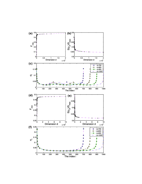
Figure 2: (Color online)The violation illustration of the CGLMP inequality in the $d$-dimensional Hilbert space. (a), (b), (c) describe the negative maximal violations, while (d), (e), (f) describe the positive maximal violations.

In Fig. 2 we show numerically the maximal violations up to $d=10^{6}$ for positively maximal violations and $d=2\times 10^{5}$ for negatively maximal violations. It is seen from Fig. 2(a)(d) that the strength of quantum nonlocality denoted by $F_{\min}$ have a decelerating increase with the growing system dimension $d$ and it approaches a finite maximal value when $d$ goes to infinity. The increasing trend also shows a stronger quantum nonlocality in a higher dimensional system. An interesting phenomenon is that although the quantum nonlocality becomes stronger in a higher dimensional system, the corresponding state, from Fig 2.(b)(e), has a decreasing entangled degree and hence deviates farther from the most entangled state. From Fig. 2(c)(f), these Schmidt coefficients of states corresponding those maximal quantum violations have a symmetric distribution and they obey the same pattern no matter how big the dimension is. By comparing Fig. 2(a-c) with Fig. 2(d-f), there are several differences between the positively and negatively maximal violations: (i) at the same dimension, the negatively maximal violation of $I_{d}$ has a little larger $F_{\min}$ than the positively maximal violation (e.g. when $d=2\times 10^{5}$, the negatively maximal violation has $F_{\min}=0.487$ while the positively maximal violation has $F_{\min}=0.477$); (ii) compared with the positively maximal side, there is a smaller deviation for the states corresponding to negatively maximal side (e.g. when $d=1\times 10^{5}$, the negatively maximal violation has $S(\rho_{A})/S_{\max}=0.848$ while the positively maximal violation has $S(\rho_{A})/S_{\max}=0.826$). Note that for $d=3$, the negative side of $I_{d}$ has no violation with $F_{\min}=0$ and so at this point it does not satisfy the above general rules.

In summary, continued with the previous paper 2006Chen , we have investigated the maximal violations of the CGLMP inequality for two $d$-dimensional systems further. The maximal violation occurs at the nonmaximally entangled state, which is the eigenvector of Bell operator with the maximal eigenvalue. Numerically, we display the maximal violating values up to $d=10^{6}$ for the positively maximal violation and $d=2\times 10^{5}$ for the negatively maximal violation. It gives us a straightforward picture on the trend of quantum nonlocality with the dimension of systems increasing. That is, the maximal violations increase as the dimension $d$ grows and approaches a finite value when $d$ becomes infinity. In addition, deviations of the entangled pure states that are in accordance with maximal violations from maximally entangled states have also been discussed. It is shown that as the dimension $d$ increases, the deviation also approaches some constant limit.

Particulary, by comparing the violations at both sides of $I_{d}$, we show that the negatively maximal violation has a little stronger quantum nonlocality than the positively maximal violation has. This may be counterintuitive to the previous notion that the positively maximal violation of the CGLMP inequality is enough. Also, by giving out the phase rules and the elements of the Bell operator matrix, we have in fact given a convenient way to calculate the maximal violation of the CGLMP inequality on its both sides. It can serve as a useful reference for experimental setting when testing the CGLMP inequality. The experimental test has been performed to verify the CGLMP inequality for the first few high-dimensional systems 2002Vaziri , and it shows that indeed there exist nonmaximally entangled states violating the inequality more strongly than the maximal entangled ones . Thus, the nonmaximally entangled states in high-dimensional quantum systems as discussed in this paper may turn to be comparably useful when applied to quantum cryptography and quantum communication complexity 1991Ekert ; 2003Kasz ; 2004Durt ; 2002Brukner ; 2004Brukner , in which previous researches are mostly based on maximally entangled states.

Figure legends

Figure 1: The diagram of unbiased multiport beam splitter. In front of the $i$th input port of the device a phase shifter is placed to change the phase of the incoming photon by $\phi(i)$. The whole action can be described by unitary operator $U(\hat{\phi}_{a})$ and $U(\hat{\varphi}_{b})$.

Figure 2: (Color online)The violation illustration of the CGLMP inequality in the $d$-dimensional Hilbert space. (a), (b), (c) describe the negative maximal violations, while (d), (e), (f) describe the positive maximal violations.

Figures

Figure 1

Figure 2