Generalized MSTB Models:
Structure and kink varieties.

Abstract

In this paper we describe the structure of a class of two-component scalar field models in a (1+1) Minkowskian space-time which generalize the well-known Montonen-Sarker-Trullinger-Bishop -hence MSTB- model. This class includes all the field models whose static field equations are equivalent to the Newton equations of two-dimensional type I Liouville mechanical systems with a discrete set of instability points. We offer a systematic procedure to characterize these models and to identify the solitary wave or kink solutions as homoclinic or heteroclinic trajectories in the analogous mechanical system. This procedure is applied to a one-parametric family of generalized MSTB models with a degree-eight polynomial as potential energy density.

1 Introduction

Over the last decades topological defects or solitary waves have played an essential r$\hat{\rm o}$le in the explanation of new phenomena in diverse branches of Science, e.g., Cosmology and Condensed Matter Physics. These non-linear waves are non-dispersive spatially localized solutions of non-linear field equations describing a given physical system. Focusing on one-dimensional wave phenomena, we shall deal with variations of the relativistic non-linear Klein-Gordon PDE [2]

$$\frac{\partial^{2}\phi_{a}}{\partial t^{2}}-\frac{\partial^{2}\phi_{a}}{\partial x^{2}}+\frac{\partial U}{\partial\phi_{a}}=0\hskip 56.9055pta=1,\dots,N$$ (1)

for $N$ scalar fields $\phi_{a}(x,t)$. The non-linear nature of these equations is the key point to finding unexpected a priori non-dispersive wave solutions. The simplest examples of relativistic topological defects of this kind are the soliton of sine-Gordon theory and the kink of the $(\phi)_{2}^{4}$ model. These systems encompass only one scalar field and provide theoretical support to explain, for instance, the appearance of superconductivity in type II materials [3, 4], electric charge fractionization in trans-polyacetylene (CH)_x [5], the Josephson effect, [6], etcetera. In several branches of Physics ranging from condensed matter physics to cosmology, from fluid dynamics to relativistic quantum field theory, more complex systems involving several scalar fields arise. The search for topological defects, solitary waves or kinks in models which involve several scalar fields, as Rajaraman notices [7], is a very difficult endeavor: This already brings us to the stage where no general methods are available for obtaining all localized static solutions (kinks), given the field equations. However, some solutions, but by no means all, can be obtained for a class of such Lagrangians using a little trial and error. The move from one-component scalar field models to two-component scalar field models is thus a very important qualitative step, passing from the integration of a single partial differential equation to the integration of a system of partial differential equations. Although there are no general methods to tackle the problem of solving systems of non-linear partial differential equations, some strategies for finding soliton solutions have been developed in both the physical and mathematical literature over the last thirty years.

We now point out two of these strategies that lie at the core of the conceptual framework to be developed in this paper:

• Since the models we are interested in exhibit Lorentz invariance, see (1), the search for kinks or traveling waves is tantamount to the solution of an analogous mechanical problem where the unit-mass point particle motion in a certain potential $V(\phi_{1},\phi_{2})$ must be identified: this analogy is established by thinking of the variable $x$ as “time” whereas the field components $(\phi_{1},\phi_{2})$ are reinterpreted as the coordinates of the particle [7] moving in the Euclidean plane under the influence of the potential $V(\phi_{1},\phi_{2})=-U(\phi_{1},\phi_{2})$. Moreover, the field theoretical energy becomes the mechanical action. This identification means that finite energy field configurations correspond to finite action (in infinite time) paths in the analogous mechanical system.

  By this token one must solve only a system of ordinary differential equations, instead of partial differential equations. Traveling wave solutions to the PDE system are thus obtained by applying Lorentz transformations (or Galilean, in non-relativistic systems) to the static solutions of the ODE system.

• In some models the potential density energy can be written as half the square of the norm of the gradient of a “superpotential” $W(\phi_{1},\phi_{2})$:

  $$U(\phi_{1},\phi_{2})={1\over 2}\left(\frac{\partial W}{\partial\phi_{1}}\cdot\,\frac{\partial W}{\partial\phi_{1}}+\frac{\partial W}{\partial\phi_{2}}\cdot\,\frac{\partial W}{\partial\phi_{2}}\right)\qquad.$$ (2)

  Knowledge of such a function, $W(\phi_{1},\phi_{2})$, allows the Bogomolny’i-Prasad-Sommerfield arrangement [8] for the energy functional:

  $$E[\phi_{1},\phi_{2}]=\frac{1}{2}\int dx\sum_{a=1}^{2}\left[\frac{d\phi_{a}}{dx}-\frac{\partial W}{\partial\phi_{a}}\right]^{2}+\int dx\sum_{a=1}^{2}\frac{\partial W}{\partial\phi_{a}}\frac{d\phi_{a}}{dx}\qquad.$$ (3)

  Because it is an exact differential if $W$ is well behaved, the second term

  $$T=\int_{\mathbb{R}}dx\sum_{a=1}^{2}\frac{\partial W}{\partial\phi_{a}}\frac{d\phi_{a}}{dx}=\int_{\mathbb{K}}\,dW\qquad,\qquad{\mathbb{K}}:{\mathbb{R}}\longrightarrow{\mathbb{R}}^{2}\qquad,$$

  where by ${\mathbb{K}}(x)\in Maps({\mathbb{R}},{\mathbb{R}}^{2})$ we denote a non-singular curve in ${\mathbb{R}}^{2}$, in (3) only depends on the values of $W$ at the end points of the curve: $W[\phi_{1}(\pm\infty,t),\phi_{2}(\pm\infty,t)]$. If finite energy is required, the following conditions at spatial infinity, $\partial{\mathbb{R}}$, must be satisfied:

  $$(\phi_{1}(\pm\infty,t),\phi_{2}(\pm\infty,t))\in{\cal M}\qquad,\qquad\frac{d\phi_{1}}{dx}(\pm\infty,t)=0=\frac{d\phi_{2}}{dx}(\pm\infty,t)\qquad,$$

  where ${\cal M}$ is the set of zeroes of $U$, assuming a non-negative $U$. Because the temporal evolution is a homotopy transformation, when ${\cal M}$ is a discrete set $W[\phi_{1}(\pm\infty,t),\phi_{2}(\pm\infty,t)]$ is time-independent, and $T$ is a “topological charge”.

  The second term in (3) is semi-definite positive and the absolute minima of the energy are solutions of the first-order system of ordinary differential equations:

  $$\frac{d\phi_{a}}{dx}=\frac{\partial W}{\partial\phi_{a}}\hskip 28.45274pt,\hskip 56.9055pta=1,2\qquad.$$ (4)

  Non-dispersive extended solutions of (4) are also stable solutions of the second-order ODE system (5) obeying the static field equations:

  $$\frac{d^{2}\phi_{a}}{dx^{2}}=\frac{\partial U}{\partial\phi_{a}}\hskip 85.35826pt,$$ (5)

  usually referred to as solitary waves, kinks, or one-dimensional topological defects.

  The link between these two strategies is hidden in equation (2). This equation is no more than the reduced Hamilton-Jacobi equation for zero mechanical energy trajectories of the analogous mechanical system. As a consequence $W$ is the Hamilton characteristic function, whereas the term superpotential comes from the fact that only models with potential energy of the form written in (2) are susceptible to supersymmetric extensions.

  In this way, the search for solitary waves in $N$ scalar field theory is tantamount to the solving of a $N$-dimensional mechanical system. Thus, the most favorable situation is to deal with integrable mechanical systems. If $N=2$, there is a lot of information about classes of integrable mechanical systems, see e.g. [42]. In particular, we shall choose field theoretical models such that their analogous mechanical system is of Liouville Type I: those two-dimensional mechanical systems such that their Hamilton-Jacobi equation is separable using elliptic coordinates. The simplest and best studied (1+1) dimensional two-component scalar field theory model of this type is the MSTB model (after Montonen, Sarker, Trullinger and Bishop, who first addressed this theory in [18, 19]).

  Our goal in this paper is to analyze the structure of this broad class of systems of the MSTB (the tip of the iceberg) type as well as to study their manifold of solitary waves. Applications of multi-component kinks to describe interesting physical systems abound in the literature, see [7-15].

1.1 The MSTB Model

The MSTB model is a physical system with a proud history. In 1976 Montonen [18], searching for charged solitons in a model with one complex and one real scalar field, discovered, by fixing the time-dependent phase for the complex field, a (1+1)-dimensional two real scalar field theory that provided the basic neutral solitons. When such basic neutral solitons are embedded in the bigger system charged solitons arises. Thus, the MSTB model is a (1+1)-dimensional relativistic theory of two scalar fields with potential energy density:

$$U_{\rm MSTB}[\phi_{1}(x,t),\phi_{2}(x,t)]=\frac{1}{2}(\phi_{1}^{2}(x,t)+\phi_{2}^{2}(x,t)-1)^{2}+\frac{\Omega^{2}}{2}\phi_{2}^{2}(x,t)\qquad.$$ (6)

Considered as a function of the two scalar fields $\phi_{1}$ and $\phi_{2}$, $U_{\rm MSTB}$ is a fourth-order polynomial isotropic in quartic but anisotropic in quadratic terms. There is only one non-dimensional parameter $\Omega$, which determines the intensity of the anisotropy (as well as the time dependence of the phase of the complex scalar field).

The kink solutions asymptotically connect elements of the set of zeroes of $U_{\rm MSTB}(\phi_{1},\phi_{2})$, which in this case are two : ${\cal M}=\{(\phi_{1}^{+}=1,\phi_{2}^{+}=0);\,(\phi_{1}^{-}=-1,\phi_{2}^{-}=0)\}$. In his seminal paper [18], the author identified two solitary waves or kinks, joining the points $\phi_{+}$ and $\phi_{-}$ asymptotically in the range of the coupling constant: $\Omega^{2}\in(0,1)$. The first kink was the old kink of the $\phi^{4}_{2}$ theory with only one real scalar field:

$$\phi_{1}^{\rm TK1}(x)=\tanh\bar{x}\hskip 28.45274pt,\hskip 28.45274pt\phi^{\rm TK1}_{2}(x)=0\qquad;\qquad\bar{x}=\frac{(-1)^{\alpha}(x-\gamma_{2})-vt}{\sqrt{1-v^{2}}}$$ (7)

where $\alpha=0,1$, $v$ is a velocity slower than the speed of light $c=1$, and $\gamma_{2}\in\mathbb{R}$ sets the kink center, see Figure 1. The dependence on $\bar{x}$ is due to the breaking of the translational, Lorentz, and reflection symmetries of the model by the kink solution. Because the second field is zero for this solution, it is referred to with the abbreviated name of TK1 kink (one-component topological kink): the topological charge is non-zero and only one field component is non-null, whereas the solution lives in the abscissa axis of the ${\mathbb{R}}^{2}$ field space, tracing the orbit: $(\phi^{\rm TK1}_{1}\in(-1,1),\phi^{\rm TK1}_{2}=0)$, which starts and ends at different points of ${\cal M}$.

The second and novel kink connects the points $\phi^{+}$ and $\phi^{-}$ through the semi-elliptic orbits

$$\phi_{1}^{2}+\frac{\phi_{2}^{2}}{{\bar{\Omega}}^{2}}=1\qquad\qquad,\qquad\bar{\Omega}^{2}=1-\Omega^{2}$$ (8)

in the ${\mathbb{R}}^{2}$ field space. Solitary wave solutions of this type read:

$$\phi_{1}^{\rm TK2}(\bar{x})=\tanh\Omega\bar{x}\hskip 28.45274pt,\hskip 28.45274pt\phi_{2}^{\rm TK2}(\bar{x})=(-1)^{\beta}\bar{\Omega}\,{\rm sech}\,\Omega\bar{x}\qquad;\qquad\beta=0,1\quad,$$ (9)

see Figure 1. The abbreviated name for solitary waves of this type is ${\rm TK2}$ kink (two-component topological kinks) because the topological charge is not zero and the two field components are non-null. It is clear that (8) becomes a hyperbola when $\Omega^{2}>1$ and ${\rm TK2}$ kinks do not exist in this range. ${\rm TK1}$ kinks, however, are still traveling wave solutions for $\Omega>1$.

To be precise, in a previous paper [20] Rajaraman and Weinberg had identified the first class of these solutions and had described the qualitative behavior of the second type of kinks in a more general model. Sarker, Trullinger, and Bishop entered the game by establishing the stability of the two kinds of solution from a energetic point of view [19]: if $\Omega^{2}\in(0,1)$ the TK2 kinks, being less energetic, are the stable traveling wave solutions and the TK1 kinks should decay to them. If $\Omega^{2}>1$, obviously the TK1 kinks are stable. In 1979, further analysis of kink stability in this model were performed in References [21] and [22]. Study of the spectrum of the second-order small fluctuation operator around ${\rm TK1}$ and ${\rm TK2}$ kinks confirmed that the latter are stable and the former unstable. The lowest eigenvalue is positive (respectively, negative) for ${\rm TK2}$ (respectively,${\rm TK1}$) kinks if $\Omega^{2}<1$, and positive for ${\rm TK1}$ kinks if $\Omega^{2}>1$.

In the same year, Rajaraman [23] discovered a new kind of kink solution for the particular value of the coupling constant $\Omega=\frac{1}{2}$ whose orbits are the circle trajectories:

$$(\phi_{1}\mp\frac{1}{4})^{2}+\phi_{2}^{2}=\frac{9}{16}\qquad\qquad.$$

These ${\rm NTK2}$ kink solutions read

$$\phi_{1}^{\rm NTK2}(x)=\pm\frac{3}{2}\tanh^{2}\frac{\bar{x}}{2}\mp\frac{1}{2}\hskip 56.9055pt\phi_{2}^{\rm NTK2}(x)=\frac{3}{2}\,{\rm sech}\,\frac{\bar{x}}{2}\tanh\frac{\bar{x}}{2}$$

and asymptotically reach $\phi^{+}$ , or, $\phi^{-}$ both at $x=\pm\infty$, see Figure 1. Hence, these solitary waves are referred to as two-component non-topological kinks, or, ${\rm NTK2}$ kinks.

                   

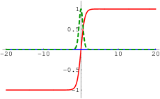
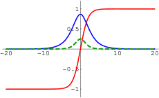
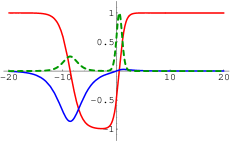
Figure 1: $\phi_{1}^{K}$ profile (red solid lines), $\phi_{2}^{K}$ profile (blue solid lines), and energy density (green dashed lines) of the TK1, TK2 and NTK2 kinks in the MSTB model.

The discovery of this new type of solitary wave prompted several numerical investigations by Subbaswamy and Trullinger; their research focused on numerical explorations of the existence, energy, and stability of non-topological kink solutions in a wide range of $\Omega$ [24, 25]. These authors numerically found that there exists a continuous family of non-topological kinks of NTK2 type that describe closed orbits, all of them enclosed by the ellipse (8) in the field space ${\mathbb{R}}^{2}$ if $\Omega^{2}\in(0,1)$. Moreover, they numerically checked an astonishing but simple relationship between kink energies: the energy of any of the non-topological kinks is the sum of the energies of the two topological kinks:

$$E[{\rm NTK2}]=E[{\rm TK1}]+E[{\rm TK2}]\qquad\qquad.$$ (10)

This identity, termed the kink mass sum rule, was regarded as a mysterious property of the model (consider the kink energy densities in Figure 1). In 1984, Magyari and Thomas [26] noticed a very important feature of the model: by finding a second constant of motion, in involution with the mechanical energy, these authors showed that the two-dimensional analogous mechanical system is completely integrable. In fact, the analogous mechanical model is a particular case of the Garnier integrable system, see [27]. Having two isolated unstable points -the minima of $U$ are the maxima of $V$- of maximum potential energy, the heteroclinic trajectories of finite mechanical action joining those points are precisely the topological kinks. Homoclinic trajectories, however, starting from and ending at the same maximum correspond to the non-topological kinks. The intelligence of this fact plus the existence of two invariants in involution provided an strong hint about the origin of the kink mass sum rule as being due to continuous degeneracy in the mechanical action of all the separatrix trajectories sharing the critical values of the two constants of motion.

In 1985, Ito [28] showed that the analogous mechanical system is not only completely integrable but Hamilton-Jacobi separable by using elliptic coordinates. The immediate application by Ito of the Hamilton-Jacobi principle allowed him to describe the whole kink orbit and kink profile varieties analytically by means of complicated expressions between elliptic variables. In particular, he verified the sum rule by analytically checking that all the closed trajectories have the same mechanical action.

Although to the best of our knowledge nobody has been able to invert Ito’s implicit expressions, we recently succeed in doing this by performing a shrewd reshuffling of the kink orbit equations, to find:

$$\phi_{1}^{\rm NTK2}(\bar{x};\gamma_{1}) = \frac{(\Omega-1)(1+e^{2(1+\Omega)(\bar{x}+\Omega\gamma_{1})})+(\Omega+1)(e^{2\Omega(\bar{x}+\gamma_{1})}+e^{2(\bar{x}+\gamma_{1}\Omega^{2})})}{(\Omega-1)(1+e^{2(1+\Omega)(\bar{x}+\Omega\gamma_{1})})-(\Omega+1)(e^{2\Omega(\bar{x}+\gamma_{1})}+e^{2(\bar{x}+\gamma_{1}\Omega^{2})})}$$

$$\phi_{2}^{\rm NTK2}(\bar{x};\gamma_{1}) = \frac{2(\Omega^{2}-1)e^{\Omega(\bar{x}+\gamma_{1})}(e^{2(\bar{x}+\gamma_{1}\Omega^{2})}-1)}{(\Omega-1)(1+e^{2(1+\Omega)(\bar{x}+\Omega\gamma_{1})})-(\Omega+1)(e^{2\Omega(\bar{x}+\gamma_{1})}+e^{2(\bar{x}+\gamma_{1}\Omega^{2})})}\qquad.$$ (11)

This one-parametric family of solitary waves, depending on the real integration constant $\gamma_{1}\in\mathbb{R}$, is the whole manifold of two-component non-topological kinks of the model.

Next, Ito and Tasaki [2] addressed the issue of the kink stability of the kink solutions from a very interesting point of view: applying the Morse index theorem to the kink orbits they showed that the unique stable kink in the $\Omega^{2}<1$ range is the TK2 kink. These authors realized that all the other kink orbits starting from one of the vacuum points pass through one of the two foci $\phi^{f_{\pm}}=(\phi_{1}^{f_{\pm}}=\pm\Omega,\phi_{2}^{f_{\pm}}=0)$ of the ellipse (8); these points are thus respectively conjugate to one of the two unstable points $\phi_{\pm}=(\phi^{1}_{\pm}=\pm 1,\phi^{2}_{\pm}=0)$ because each kink orbit starting from $\phi_{-}$ (respectively $\phi_{+}$) passes through $\phi^{f_{+}}$ (respectively $\phi^{f_{-}}$). In Reference [29] Guilarte extended this idea to embedding the kink stability problem in the degenerate Morse theory of the configuration space, bearing in mind that, in this framework, the topology of an infinite dimensional manifold -the configuration space of the MSTB model- is determined from the critical points -the kinks- of a functional -the energy of the MSTB model-. A full analysis of this approach was achieved in Reference [30], where the Morse’s Lemma, governing the small fluctuations around the kink solutions, suggests how to deal with quantum corrections. This goal was fully attained from this point of view in Reference [31]. To finish this subsection about the history of the MSTB model, let us mention that in [32] the decay amplitude from the TK1 to the TK2 kink was computed in the quantum MSTB model by using the Witten-Smale version of Morse theory.

Two properties of the kink variety of the MSTB model induced its early perception as singular and unique: a) The existence of several kinds of kink: the TK1 kink, the TK2 kink and the NTK2$(\gamma_{1})$ kink family. b) The relationship between its energies (the kink mass sum rule).

1.2 The discovery of new models of the MSTB type

The critical feature of the MSTB model allowing this perception to be overcome is the fact that its analogous mechanical system is an integrable system of Liouville type. In [33] Alonso, Gonzalez, and Guilarte proposed and studied two models of the MSTB kind with different potential energy densities, chosen in such a way that their analogous mechanical system would be of Type I in the first model and Type III Liouville integrable system in the second case. Together with a selection of parameters ensuring the existence of a discrete set of maxima for the mechanical potential -five in the first, four in the second model- this work revealed for the first time that the MSTB is by no means unique but, rather, a member of a broad family of models. The configuration space is formed by $25$ (in the first case) and $16$ (in the second model) topologically disconnected sectors and it is expected that the kink varieties in these cases will be richer than in the MSTB system. This is indeed the case, and several families of stable and unstable topological kinks were discovered with various new kink mass sum rules arising between the different kink types.

Model B, the second model in [33], is Liouville Type III, i.e., its analogous mechanical system is a two-dimensional Hamilton-Jacobi separable system in parabolic coordinates. Remarkably, this system arises for a particular value of the coupling constant of a model that is important in supersymmetric field theory. The dimensionally reduced Wess-Zumino model discussed by Bazeia et al. in [10, 11] is not in general of Liouville Type. Only for two special values of the coupling constant does the analogous mechanical system fall into this class: one of the values leads to a mechanical system of Type III already mentioned, and the other one gives a Liouville system of Type IV, Hamilton-Jacobi separable in Cartesian coordinates. The important point is that, given its supersymmetric origin, a solution of the Hamilton-Jacobi equation (not complete) is always known and trajectories associated to this solution (the superpotential) can be found. This strategy was used in [34] to find a whole family of topological kinks in the BNRT (acronym from [11], in analogy with the MSTB acronym from [18] and [19]) model. The difference with model B, a particular case, is the HJ-separability that allows one to know a complete solution of the Hamilton-Jacobi equation and, therefore, knowledge of all the trajectories. The point is that for models with analogous mechanical system of Liouville Type, complete integrability permits an exhaustive knowledge of all the kink orbits, which, in turn, provides a full understanding of the solitary wave manifold and kink mass sum rules between them. Recently, this analysis has been performed in [35] for some Type II Liouville systems; the field theoretical models analyzed have analogous mechanical systems HJ separable in polar coordinates.

A general pattern emerges from the study of the manifold of kink solutions in these models. There are two kinds of solitary waves: basic kinks with energy density localized at one point in ${\mathbb{R}}$ and families of composite kinks, non-linear superpositions of several basic kinks, such that their energy densities are localized at several points in ${\mathbb{R}}$. The distance between the basic lumps of energy is determined by the parameter fixing the corresponding kink orbit. The situation is perfectly illustrated in Figure 1. By using a solid line in the three graphics we represent the profile of the three kinds of solution in the MSTB model, i.e, the TK1, the TK2 and a member of the NTK2 family of kinks respectively. We also depict the energy density of these solutions by using a dashed line. We notice that the energy density of the TK1 and TK2 kinks are localized around one point while the energy density for the NTK2 kink is localized around two points. The NTK2 is composed of the other two kinks. The parameter $\gamma_{1}$ in (11) fixes the distance between the TK1 and TK2 kinks. In References [36, 37] a description of the evolution of this distance in time has been worked out for slow speeds. Although we are dealing with non-linear systems, the adiabatic evolution of composite kinks can be dealt with as geodesic motion in the kink parameter space with respect to the metric induced by the field kinetic energy density, thus providing a good description of kink scattering at low energies. From this point of view, kink mass sum rules become natural: these rules are forced by energy conservation when radiative processes are absent, i.e., the energy of a composite kink is the sum of the energies of the component basic kinks.

One might wonder at this point if similar structures arise in systems with more scalar fields. In References [38, 40] a positive answer addressing field theoretical systems with three scalar fields was found. The analysis is even more difficult, because three-dimensional Hamilton-Jacobi separable systems not abound. Now, the composite kinks are formed by three basic kinks. Stability issues are also more difficult to deal with, although in [39] a thorough study of kink stability was achieved in the generalization of the MSTB model to three fields. The adiabatic dynamics of three slow moving kinks has also been recently unveiled in [41].

1.3 Generalized MSTB Models

The work in the papers referred to above shows that the MSTB model is not a unique or special model. Several models are known to share essential characteristics with the MSTB model, in such a way that the kink variety of each model and its properties can be identified by a parallel analysis. Our goal in this paper is to study the general structure of this type of models, which we shall call generalized MSTB models. All these systems share the same critical properties: their analogous mechanical system is a Type I Liouville system having a discrete set of maxima in the mechanical potential energy; these MSTB-type models are distinguished by the number of zeroes -the maxima- of the non-positive mechanical potential energy. The kink variety can always be identified as the manifold of separatrix trajectories between the bounded and unbounded motion of the integrable mechanical system of Liouville Type I. Remarkably, the structure of the kink variety can be unveiled in all of these models without solving any OD equation. Moreover, the kink mass sum rules can also be guessed simply from the analytical form of the potential density energy.

This paper is organized as follows: In Section §. 2 we shall define generalized MSTB models as field theoretical two scalar field models with analogous mechanical system of Liouville Type I. These two-dimensional mechanical systems are Hamilton-Jacobi separable in elliptic coordinates. Thus, in this Section, we shall translate the generalized MSTB models into elliptic coordinates, mapping the internal field space ${\mathbb{R}}^{2}$ to the infinite strip ${\mathbb{E}}^{2}\equiv{\mathbb{R}}^{+}\times{\mathbb{I}}\equiv\,\,[\Omega,+\infty)\times[-\Omega,\Omega]$, where $\Omega\in(0,1)$ is a real number between $0$ and $1$. In Section §. 3 we shall study the kink manifold that arises in this kind of model. In order to do this, the distribution of the zeroes of the potential energy density is crucial. In generalized MSTB models these zeroes are located at the nodes of a grid or reticulum in the “elliptic strip” ${\mathbb{E}}^{2}$. The distribution of zeroes of the potential determines the classification of generalized MSTB models in four types. Generically, the reticulum is formed by gluing several cells where the kinks are confined. The zeroes of the potential energy density live at the vertices of the cells and/or at the foci of the elliptic and hyperbolic curves that set the curvilinear coordinate system. There are three types of cells distinguished by the nature of the vertices. The type of cell determines the behavior of the kink family confined in the cell. In general, there are basic and isolated kinks living in the bars of the grid surrounding the cell and families of kinks living inside. Each member of one of these families is a non-linear superposition of basic kinks: these are composite kinks and have their energy density localized around several points, each of these component lumps having the same energy density as a basic kink. In this Section, we shall also explore new and generalized kink mass sum rules and we shall investigate the relationship between the integrability of the analogous mechanical systems and the existence of superpotentials. In Section §. 4 we shall describe the kink variety of a specific model. The MSTB model [18] involves a quartic algebraic potential energy density, whereas the potential energy density of model A in [37] is a polynomial in the fields of sixth degree. In order to deal with completely new generalized MSTB models, we shall analyze a model characterized by a eighth degree polynomial in the two fields as the potential energy density. The polynomial depends on two coupling constants in such a way that a process of bifurcation arises: the number of elements in ${\cal M}$, static homogeneous solutions of the field theoretical model or the fixed points of the Newton equations of the analogous mechanical system, depends on the values of the coupling constants. There are three regimes where we shall study the kinks and also the kink mass sum rules. Finally, the summary of the main results and the outlook on future research in similar models are offered in Section §. 5.

2 The structure of generalized MSTB models

2.1 The configuration space

We shall study field theoretical models of two real scalar fields defined in a (1+1) Minkowskian space-time, whose dynamics is governed by the action functional:

$$S[\vec{\phi}]=\int dxdt\left[\frac{1}{2}\sum_{a=1}^{2}\partial^{\mu}\phi_{a}\partial_{\mu}\phi_{a}-U(\phi_{1},\phi_{2})\right]\qquad.$$ (12)

We use Einstein sum convention for Greek scripts and choose the metric tensor to be: $g_{00}=-g_{11}=1$, $g_{01}=g_{10}=0$. By $\vec{\phi}=\sum_{a=1}^{2}\phi_{a}\vec{e}_{a}$, $a=1,2$, we denote the scalar fields:

$$\vec{\phi}(x_{0},x_{1})=\phi_{1}(x_{0},x_{1})\vec{e}_{1}+\phi_{2}(x_{0},x_{1})\vec{e}_{2}:\mathbb{R}^{1,1}\rightarrow\mathbb{R}^{2}$$

The vectors $\vec{e}$ form an orthonormal basis in ${\mathbb{R}}^{2}$ and $U(\phi_{1},\phi_{2})$ is the (non-negative) potential energy density, which vanishes in a discrete set of points, ${\cal M}$. For the sake of simplicity we assume that the magnitudes involved in (12) are dimensionless.

A point in the configuration space of the system is a configuration of the field of finite energy; i.e., a picture of the field at a fixed time such that the energy $E$, the integral over the line of the energy density,

$$E[\vec{\phi}]=\int_{-\infty}^{\infty}dx\,{\cal E}[\vec{\phi}(x)]\hskip 28.45274pt;\hskip 28.45274pt{\cal E}[\vec{\phi}(x)]=\frac{1}{2}\left(\frac{d\phi_{1}}{dx}\right)^{2}+\frac{1}{2}\left(\frac{d\phi_{2}}{dx}\right)^{2}+U(\phi_{1},\phi_{2})$$ (13)

is finite. Therefore, the configuration space is the set of continuous maps from $\mathbb{R}$ to $\mathbb{R}^{2}$ of finite energy:

$${\cal C}=\{\vec{\phi}(x)\in{\rm Maps}(\mathbb{R},\mathbb{R}^{2})\,/\,E[\phi]<\infty\}$$

In order to belong to ${\cal C}$, each configuration must comply with the asymptotic conditions

$$\lim_{x\rightarrow\pm\infty}\vec{\phi}(x)\in{\cal M}\hskip 56.9055pt,\hskip 56.9055pt\lim_{x\rightarrow\pm\infty}\frac{d\vec{\phi}}{dx}=0$$ (14)

where ${\cal M}$ is the set of zeroes of the potential energy density $U(\phi)$,

$${\cal M}=\{\vec{\phi}^{(I)}\in\mathbb{R}^{2}\subset{\rm Maps}(\mathbb{R},\mathbb{R}^{2})\,/\,U[\vec{\phi}^{(I)}]=0\,\,,\,\,I=1,2,\cdots,N\}\qquad.$$

We shall also choose $U(\vec{\phi})$ non-negative and such that ${\cal M}$ is also the set of absolute minima of $U$, i.e., the set of the static homogeneous solutions of the model because the Euler-Lagrange field equations of (12)

$$\frac{\partial^{2}\phi_{a}}{\partial t^{2}}-\frac{\partial^{2}\phi_{a}}{\partial x^{2}}+\frac{\partial U}{\partial\phi_{a}}=0\hskip 28.45274pt,\qquad a=1,2$$ (15)

are satisfied by the elements of ${\cal M}$. Moreover, bearing in mind that time evolution is continuous -a homotopy transformation-, if ${\cal M}$ is a discrete set the configuration space is the union of disconnected topologically sectors ${\cal C}^{IJ}$:

$${\cal C}=\bigcup_{I,J\in{\cal M}}{\cal C}^{IJ}\qquad.$$

The configurations in ${\cal C}^{IJ}$ are characterized as those which respectively tend to the elements $\vec{\phi}^{(I)}$ and $\vec{\phi}^{(J)}$ of ${\cal M}$ at minus and plus spatial infinity.

According to Rajaraman [7]: A kink is a non-singular solution of non-linear field equations (15) whose energy density, as well as being localized, has space-time dependence of the form: $\varepsilon(t,x)=\varepsilon(x-\rm{v}t)$, where v is some velocity vector. Because we are dealing with a Lorentz invariant system, solutions with a temporal dependence like this are obtained from static solutions by means of a Lorentz velocity transformation: $L({\rm v})\phi(x)=\phi^{L}(t,x)=\phi\left(\frac{x-{\rm v}t}{\sqrt{1-{\rm v}^{2}}}\right)$. Bearing this in mind the PDE (15) can be restricted to the ODE

$$\frac{d^{2}\phi_{a}}{dx^{2}}=\frac{\partial U}{\partial\phi_{a}}\hskip 14.22636pt,\hskip 14.22636pta=1,2\hskip 22.76228pt\equiv\hskip 22.76228pt\frac{d^{2}\vec{\phi}}{dx^{2}}=\vec{\nabla}U\qquad.$$ (16)

in such a way that the search for some kinks or solitary waves is tantamount to studying an analogous mechanical system, where we interpret the static scalar field $\vec{\phi}(x)=\phi_{1}(x)\vec{e}_{1}+\phi_{2}(x)\vec{e}_{2}$ as the particle position vector; $x$ as the particle time, and $U=-V$ as the particle potential. Moreover, the action and the Lagrangian of the mechanical system respectively play the r$\hat{\rm o}$les of the energy functional and the energy density in the field theory, see (13). In sum, solitary waves or kinks are derived from stationary points of the functional energy (13) that comply with the asymptotic conditions (14). Therefore, kinks asymptotically connect two elements of ${\cal M}$ or, homogeneous solutions of (16).

2.2 Algebraic Type I Liouville potentials

The potential energy density of the MSTB model is a positive quartic algebraic expression in the fields, see (6). In this sub-Section we shall characterize all the algebraic (polynomial) potential energy densities that have Type I Liouville systems as the analogous mechanical model. Because the polynomials will in general be of higher order than four, the cardinal of ${\cal M}$ may be greater than in the MSTB model, promising richer kink varieties.

Proposition 1: All the members in the ($q+2$)-parametric family of models with algebraic energy density of the form:

$$U_{q}(\phi_{1},\phi_{2})=\sum_{n=0}^{q}b_{n}\prod_{j=1}^{n}\left(\phi_{1}^{2}+\phi_{2}^{2}-2\Omega\phi_{1}\cos\frac{j\pi}{n+1}+\Omega^{2}\right)\qquad,$$ (17)

a polynomial in the $\phi_{1}$ and $\phi_{2}$ fields of degree $2q$, have analogous mechanical systems that are of Liouville Type I, [42], and, therefore, these mechanical systems are Hamilton-Jacobi separable in a system of elliptic coordinates.

The proposition will be proved later in this sub-Section. In formula (17) $b_{n}$, $n=1,\dots,q$ and $\Omega$ are the parameters or coupling constants distinguishing between the members of the family. In order to support kinks/solitary waves, or non-trivial separatrix trajectories in the analogous mechanical system, the choice of $b_{n}$ parameters must be restricted in such a way that $U(\phi_{1},\phi_{2})$ must be bounded below by a discrete degenerate set of constant field configurations that are the absolute minima of $U(\phi_{1},\phi_{2})$. Also, some transformations, e.g. scaling of the space-time $\tilde{x}^{\mu}=\lambda x^{\mu}$, scaling and rotations in internal space, $\tilde{\phi}_{a}=\gamma\phi_{a}$, $\tilde{\phi}_{1}={\rm cos}\alpha\phi_{1}-{\rm sin}\alpha\phi_{2}$, $\tilde{\phi}_{2}={\rm sin}\alpha\phi_{1}+{\rm cos}\alpha\phi_{2}$ lead to equivalent models, allowing us to restrict the values of three parameters.

Arguing as Magyari and Thomas for the MSTB model in [26], we notice that the analogous mechanical system for the potential energy density (17) is completely integrable: the static field equations (16) admit two independent invariants in involution:

$$I_{1} = \frac{1}{2}\left(\frac{d\phi_{1}}{dx}\right)^{2}+\frac{1}{2}\left(\frac{d\phi_{2}}{dx}\right)^{2}-\sum_{n=0}^{q}b_{n}\prod_{j=1}^{n}\left(\phi_{1}^{2}+\phi_{2}^{2}-2\Omega\phi_{1}\cos\frac{j\pi}{n+1}+\Omega^{2}\right)\qquad,$$ (18)

$$I_{2} = \frac{1}{2}\left[\left(\phi_{1}\frac{d\phi_{2}}{dx}-\phi_{2}\frac{d\phi_{1}}{dx}\right)^{2}-\Omega^{2}\left(\frac{d\phi_{2}}{dx}\right)^{2}\right]+\sum_{n=0}^{q}b_{n}\left[-\phi_{1}^{2}\prod_{j=1}^{n-1}\left(\phi_{1}^{2}+\phi_{2}^{2}-\right.\right.$$ (19)

$$\left.\left.-2\Omega\phi_{1}\cos\frac{i\pi}{n}+\Omega^{2}\right)+\Omega^{2}\prod_{j=1}^{n}\left(\phi_{1}^{2}+\phi_{2}^{2}-2\Omega\phi_{1}\cos\frac{j\pi}{n+1}+\Omega^{2}\right)\right]$$

The first invariant is the energy of the mechanical system and the second one is also quadratic in the velocities, a certain deformation of a first-integral of Runge-Lenz type. Therefore, the field theoretical model is associated to an analogous mechanical system of Stäckel type. By choosing an appropriate system of coordinates dynamical systems of this kind are always Hamilton-Jacobi separable. The form of the second invariant dictates that elliptic coordinates will produce a separable Hamilton-Jacobi equation (Type I Liouville systems) and all the solutions can be found by quadratures. In the MSTB model, this property was used by Ito [28]) to find all the solitary wave solutions.

To study algebraic Type I Liouville systems we define Euler elliptic coordinates by means of the map:

$$\begin{array}[]{cccc}\xi_{\Omega}^{\pm}:&{\mathbb{E}}^{2}\equiv[-\Omega,\Omega]\times[\Omega,\infty)&\longrightarrow&{\mathbb{R}}^{2}/{\mathbb{Z}}_{2}\\ &(v,u)&\longrightarrow&(\phi_{1},\phi_{2})\end{array}$$

$$\xi_{\Omega}^{\pm}(u)=\frac{\sqrt{(\phi_{1}-\Omega)^{2}+\phi_{2}^{2}}+\sqrt{(\phi_{1}+\Omega)^{2}+\phi_{2}^{2}}}{2}\qquad,\qquad\xi_{\Omega}^{\pm}(v)=\frac{\sqrt{(\phi_{1}+\Omega)^{2}+\phi_{2}^{2}}-\sqrt{(\phi_{1}-\Omega)^{2}+\phi_{2}^{2}}}{2}\qquad,$$

which is a diffeomorphism between the elliptic open strip $(-\Omega,\Omega)\times(\Omega,+\infty)$ and the Cartesian upper half-plane $\phi_{2}>0$. Explicitly, the inverse map from ${\mathbb{R}}^{2}/{\mathbb{Z}}_{2}$ to ${\mathbb{E}}^{2}$, is:

$$\begin{array}[]{lcr}{\xi_{\Omega}^{\pm}}^{*}(\phi_{1})=\frac{1}{\Omega}uv&\hskip 14.22636pt,&{\xi_{\Omega}^{\pm}}^{*}(\phi_{2})=\pm\frac{1}{\Omega}\sqrt{(u^{2}-\Omega^{2})(\Omega^{2}-v^{2})}\end{array}$$ (20)

such that the coordinating curves are the hyperbolae and ellipses

$$\frac{\phi_{1}^{2}}{v^{2}}-\frac{\phi_{2}^{2}}{\Omega^{2}-v^{2}}=1\qquad\quad,\qquad\quad\frac{\phi_{1}^{2}}{u^{2}}+\frac{\phi_{2}^{2}}{u^{2}-\Omega^{2}}=1$$

whose foci are the points: $F_{\pm}=(\pm\Omega,0)$. It is necessary to use two copies of the elliptic strip ${\mathbb{E}}^{2}$ to cover the whole Cartesian internal plane: $\xi_{\Omega}^{+}$ maps ${\mathbb{E}}^{2}$ into the $\phi_{2}\geq 0$ half-plane whereas $\xi_{\Omega}^{-}$ maps the other copy of ${\mathbb{E}}^{2}$ into the $\phi_{2}\leq 0$ half-plane. Translation of information from ${\mathbb{E}}^{2}$ to the Cartesian ${\mathbb{R}}^{2}$ internal plane must take this fact into account by smoothly gluing data across the border between the two copies. In particular, the straight lines $u=\Omega$ and $v=\pm\Omega$ in ${\mathbb{E}}^{2}$ determine the axis $\phi_{1}$ in ${\mathbb{R}}^{2}$; $u=\Omega$ is the $\phi_{1}\in[-\Omega,\Omega],\phi_{2}=0$ interval and $v=\pm\Omega$ are respectively the $\phi_{1}\in[-\infty,-\Omega]$ (- sign) and $[\Omega,\infty],\phi_{2}=0$ (+ sign) half-lines, all together forming the abscissa axis in ${\mathbb{R}}^{2}$. Note that the parameter $\Omega$ setting the foci of the coordinating curves is chosen to be the coupling constant $\Omega$ in (17).

Applying the map (20) to the potential energy density (17) we obtain:

$$\xi_{\Omega}^{*}U(\phi_{1},\phi_{2}) = \frac{1}{u^{2}-v^{2}}\sum_{n=0}^{q}b_{n}\left(u^{2n+2}-v^{2n+2}\right)=\frac{1}{u^{2}-v^{2}}\left(f(u)+g(v)\right)$$ (23)

$$f:[\Omega,\infty)\rightarrow\mathbb{R}\hskip 11.38092pt;\hskip 11.38092ptu\mapsto f(u)=\displaystyle\sum_{n=0}^{q}b_{n}u^{2n+2}$$

$$g:[-\Omega,\Omega]\rightarrow\mathbb{R}\hskip 11.38092pt;\hskip 11.38092ptv\mapsto g(v)=-\displaystyle\sum_{n=0}^{q}b_{n}v^{2n+2}\qquad.$$

In elliptic coordinates the potential energy density (23) is the product of the $\frac{1}{u^{2}-v^{2}}$ factor times the sum of two polynomials, which depend only on one of the elliptic variables. $\frac{1}{u^{2}-v^{2}}$ is in all places positive in the strip ${\mathbb{E}}^{2}$ except at the foci $F_{\pm}\equiv(u,v)=(\pm\Omega,\Omega)$ (the points $(\phi_{1},\phi_{2})=(\pm\Omega,0)$ in ${\mathbb{R}}^{2}$), where the denominator vanishes. Despite this, the potential energy density is not singular at the foci $F$ because the tendency to zero is at least as strong in the numerator of (23) as in the denominator. This can be seen in the factorization:

$$u^{2n+2}-v^{2n+2}=(u^{2}-v^{2})(u^{2}-2uv\cos\frac{\pi}{n+1}+v^{2})(u^{2}-2uv\cos\frac{2\pi}{n+1}+v^{2})\cdot\dots\cdot(u^{2}-2uv\cos\frac{n\pi}{n+1}+v^{2})\,\,\,,$$ (24)

which also explains the symmetric form of the functions $f$ and $g$, i.e., $g(z)=-f(z)$. The inverse image in Cartesian coordinates of (23) provides the strange form of the potential energy density (17) $U_{q}(\phi_{1},\phi_{2})$.

The main point is that the static energy functional (13) in elliptic variables reads:

$$\xi_{\Omega}^{*}E[\phi_{1},\phi_{2}]=\int dx\left\{\frac{1}{2}\frac{u^{2}-v^{2}}{u^{2}-\Omega^{2}}\left(\frac{du}{dx}\right)^{2}+\frac{1}{2}\frac{u^{2}-v^{2}}{\Omega^{2}-v^{2}}\left(\frac{dv}{dx}\right)^{2}+\frac{f(u)+g(v)}{u^{2}-v^{2}}\right\}\qquad.$$ (25)

The functional $\xi_{\Omega}^{*}E[\phi_{1},\phi_{2}]:{\rm Maps}({\mathbb{R}},{\mathbb{E}}^{2})\longrightarrow{\mathbb{R}}$ can be interpreted as the functional action for a particle moving in ${\mathbb{E}}^{2}$ under a mechanical potential energy $V[u(x),v(x)]=-\xi_{\Omega}^{*}U[\phi_{1}(x),\phi_{2}(x)]$ if the particle time is $x$. In this conceptual framework, the change to elliptic coordinates induces a flat, but non-Euclidean, metric:

$$g^{uu}(u,v)=\frac{u^{2}-v^{2}}{u^{2}-\Omega^{2}}\qquad,\qquad g^{vv}(u,v)=\frac{u^{2}-v^{2}}{\Omega^{2}-v^{2}}\qquad,\qquad g^{uv}(u,v)=0=g^{vu}(u,v)\qquad.$$

In any case, it is well known that mechanical systems with dynamics ruled by an action such as (25) are Type I Liouville systems, see [42]. Therefore, there are two first integrals:

$$\xi_{\Omega}^{*}I_{1}=\frac{1}{2}\frac{u^{2}-v^{2}}{u^{2}-\Omega^{2}}\left(\frac{du}{dx}\right)^{2}+\frac{1}{2}\frac{u^{2}-v^{2}}{\Omega^{2}-v^{2}}\left(\frac{dv}{dx}\right)^{2}-\frac{f(u)+g(v)}{u^{2}-v^{2}}$$ (26)

$${\displaystyle\xi_{\Omega}^{*}I_{2}=\frac{1}{2}(v^{2}-u^{2})\left[\frac{\Omega^{2}-v^{2}}{u^{2}-\Omega^{2}}\left(\frac{du}{dx}\right)^{2}-\frac{u^{2}-\Omega^{2}}{\Omega^{2}-v^{2}}\left(\frac{dv}{dx}\right)^{2}\right]}{\displaystyle-\frac{(u^{2}-\Omega^{2})g(v)}{u^{2}-v^{2}}+\frac{(\Omega^{2}-v^{2})f(u)}{u^{2}-v^{2}}},$$ (27)

which allow us to solve the motion equations. Back in Cartesian coordinates, (26) and (27) become respectively (18) and (19), fully proving the Proposition.

2.3 Generalized MSTB models

Generalized MSTB models are a subset of those models having algebraic Type I Liouville systems as analogous mechanical system. In order to characterize with precision this kind of model we recall how the MSTB model arises between the $q=2$ algebraic Type I Liouville systems:

$$U_{q=2}(\phi_{1},\phi_{2}) = b_{0}+b_{1}\left(\phi_{1}^{2}+\phi_{2}^{2}-2\Omega\phi_{1}\cos\frac{\pi}{2}+\Omega^{2}\right)$$

$$+ b_{2}\left(\phi_{1}^{2}+\phi_{2}^{2}-2\Omega\phi_{1}\cos\frac{\pi}{3}+\Omega^{2}\right)\left(\phi_{1}^{2}+\phi_{2}^{2}-2\Omega\phi_{1}\cos\frac{2\pi}{3}+\Omega^{2}\right)$$

$$= a_{1}(\phi_{1}^{2}+\phi_{2}^{2}+a_{2})^{2}+a_{3}\phi_{1}^{2}+a_{4}\phi_{2}^{2}\qquad.$$

The criterion is that, up to equivalences, $U_{q=2}$ must be non-negative, having a discrete set of zeroes with more than one element; these properties give a hint of the existence of solitary waves. Demanding $U_{q=2}\geq 0$ with a discrete set of minima requires $a_{1}>0$, $a_{3}\geq 0$ and $a_{4}\geq 0$. Also $a_{1}$ can be fixed by re-scaling the space-time, $a_{2}$ by re-scalings of the fields and $a_{3}$ by rotations of the fields. In the MSTB model, we choose $a_{1}={1\over 2}$, $a_{2}=-1$, $a_{3}=0$ such that only a positive parameter, $a_{4}$, is left and there are two zeroes of $U_{q=2}$.

Another model belonging to this kinship has been dealt with in the Literature. The $q=3$ family of potential energy densities is:

$$U_{q=3}(\phi_{1},\phi_{2})=b_{0}+b_{1}\left(\phi_{1}^{2}+\phi_{2}^{2}-2\Omega\phi_{1}\cos\frac{\pi}{2}+\Omega^{2}\right)$$

$$+ b_{2}\left(\phi_{1}^{2}+\phi_{2}^{2}-2\Omega\phi_{1}\cos\frac{\pi}{3}+\Omega^{2}\right)\left(\phi_{1}^{2}+\phi_{2}^{2}-2\Omega\phi_{1}\cos\frac{2\pi}{3}+\Omega^{2}\right)$$

$$+ b_{3}\left(\phi_{1}^{2}+\phi_{2}^{2}-2\Omega\phi_{1}\cos\frac{\pi}{4}+\Omega^{2}\right)\left(\phi_{1}^{2}+\phi_{2}^{2}-2\Omega\phi_{1}\cos\frac{2\pi}{4}+\Omega^{2}\right)\left(\phi_{1}^{2}+\phi_{2}^{2}-2\Omega\phi_{1}\cos\frac{3\pi}{4}+\Omega^{2}\right)$$

$$= a_{1}(\phi_{1}^{2}+\phi_{2}^{2})^{2}(\phi_{1}^{2}+\phi_{2}^{2}+a_{2})+(a_{3}\phi_{2}^{2}+a_{4})(\phi_{1}^{2}+\phi_{2}^{2})+\frac{a_{3}(2a_{1}a_{2}+a_{3})}{4a_{1}}\phi_{2}^{2}+a_{5}\qquad.$$

$U_{q=3}$ is a five-parametric algebraic polynomial in $\phi_{1}$ and $\phi_{2}$ of sixth order that can be understood as a deformation of the Chern-Simons-Higgs potential energy density:

$$U_{\rm CSH}(\phi_{1},\phi_{2})=(\phi_{1}^{2}+\phi_{2}^{2})(\phi_{1}^{2}+\phi_{2}^{2}-1)^{2}\qquad\quad.$$

The A model investigated in Reference [37] is a special member of this family of $q=3$ with five zeroes of $U_{q=3}$. Therefore, ${\cal M}$ has five elements in the A model and the configuration space is the union of 25 disconnected topological sectors.

The potential energy densities in the MSTB (6) and A model [37] in elliptic coordinates take the form of formula (23) by choosing $f(u)$ and $g(v)$ respectively to be:

$$f(u)=\frac{1}{2}(u^{2}-1)^{2}(u^{2}-\Omega^{2})\qquad\quad \qquad\quad g(v)=\frac{1}{2}(v^{2}-1)^{2}(\Omega^{2}-v^{2})$$ ,

$$f(u)=\frac{1}{2}u^{2}(u^{2}-1)^{2}(u^{2}-\Omega^{2})\qquad\quad \qquad\quad g(v)=\frac{1}{2}v^{2}(v^{2}-1)^{2}(\Omega^{2}-v^{2})\qquad.$$ ,

Definition 1: Generalized MSTB models are (1+1)-dimensional field theoretical models of two scalar fields such that their potential energy densities have the following form in elliptic coordinates:

$$f(u)=(u^{2}-\Omega^{2})\,u^{2\alpha_{0}}\prod_{j=1}^{n+m}(u^{2}-\sigma_{j}^{2})^{2\alpha_{j}}\hskip 28.45274pt,\hskip 28.45274ptg(v)=(\Omega^{2}-v^{2})\,v^{2\alpha_{0}}\prod_{j=1}^{n+m}(v^{2}-\sigma_{j}^{2})^{2\alpha_{j}}\qquad.$$ (28)

Here $\alpha_{0},\alpha_{j},n,m\in\mathbb{N}$ are natural numbers and there are $n+m+1$ coupling constants: $\sigma_{j},j=1,2,\cdots,n+m$, and $\Omega$. With no loss of generality, we order the coupling constants in such a way that:

$$0<\sigma_{1}<\sigma_{2}<\cdots<\sigma_{n-1}<\sigma_{n}=\Omega<\sigma_{n+1}<\cdots<\sigma_{n+m}\qquad\quad.$$

This choice is guided by the following criteria:

• The potential energy density is positive for all the values of the coupling constants because all the terms involve even-power factors. Notice that the factors $(u^{2}-\Omega^{2})$ and $(\Omega^{2}-v^{2})$ in the functions $f(u)$ and $g(v)$ are semi-definite positive because of the range of the elliptic coordinates $u\in[\Omega,\infty]$ and $v\in[-\Omega,\Omega]$. The presence of these factors allows us to comply with the condition $f(z)=-g(z)$, preserving the positiveness of the potential energy density.

• The functions $f(u)$ and $g(v)$ have been also chosen in order to maximize the cardinal of the set of minima or zeroes ${\cal M}$. For this reason these functions involve only real roots. In this way the models will have a richer kink variety .

Because solitary waves come from separatrix trajectories complying with the asymptotic conditions (14), kinks will arise when $\xi_{\Omega}^{*}I_{1}=0=\xi_{\Omega}^{*}I_{2}$. Indeed the condition $\xi_{\Omega}^{*}I_{1}=0$ (26) is tantamount to the virial theorem and the kink energy density reads:

$${\cal E}[u,v]=\frac{2}{u^{2}-v^{2}}\left[f(u)+g(v)\right]=\frac{u^{2}-v^{2}}{u^{2}-\Omega^{2}}\left(\frac{du}{dx}\right)^{2}+\frac{u^{2}-v^{2}}{\Omega^{2}-v^{2}}\left(\frac{dv}{dx}\right)^{2}\qquad.$$ (29)

2.4 The structure of the set ${\cal M}$ of zeroes of $U(\phi_{1},\phi_{2})$

Bearing in mind that solitary wave solutions asymptotically connect two homogeneous minima of $U(\phi_{1},\phi_{2})$, in this sub-Section we shall study the distribution of elements of ${\cal M}$ in the internal plane ${\mathbb{R}}^{2}$. We shall show that the minima are located at the nodes of a rectangular mesh or reticulum both on the elliptic strip and on the Cartesian plane. This grid comprises a number of cells that depends on each specific model. Kinks are confined inside the cells and their qualitative behavior is determined by knowing only the type of cells where they are constrained. Moreover, on the edges of the cells single kinks emerge, while inside the cells families of composite kinks (non-linear combinations of single kinks) arise.

In order to systematize the analysis of generalized MSTB models we shall start by describing the set $\bar{{\cal M}}$ of zeroes of $\xi_{\Omega}^{*}U(\phi_{1},\phi_{2})$ on the elliptic strip ${\mathbb{E}}^{2}$. From (23), one notices that the zeroes of the potential energy density are roots of the functions $f(u)$ and $g(v)$. We shall denote respectively by

$$\bar{\cal M}_{g}=\{v\in[-\Omega,\Omega]\,/\,g(v)=0\}\hskip 28.45274pt\mbox{and}\hskip 28.45274pt\bar{\cal M}_{f}=\{u\in[\Omega,\infty)\,/\,f(u)=0\}$$

the sets of real roots of $g(v)$ and $f(u)$. We stress the following points about the elements of $\bar{\cal M}_{g}$ and $\bar{\cal M}_{f}$:

• If $\sigma_{j}$ is a root of $g(v)$, $-\sigma_{j}$ is another root, see formula (28). We shall simply denote: $\sigma_{-j}=-\sigma_{j}$.

• Although $f(u)$ and $g(v)$ are almost identical functions their domains are different: the domain of $g$ is a finite interval, ${\rm Dom}\,g=[-\Omega,\Omega]$, whereas the domain of $f$ is the infinite half-line, ${\rm Dom}\,f=[\Omega,\infty)$. For this reason, in general the numbers of roots of these functions are also different. We shall denote by $n$ and $m+1$, respectively the number of positive roots of $g(v)$ and $f(u)$. Therefore, ${\rm card}\,\bar{\cal M}_{f}=m+1$ and, either ${\rm card}\,\bar{\cal M}_{g}=2n+1$ if $v=0$ is a root of $g(v)$, or, ${\rm card}\,\bar{\cal M}_{g}=2n$ if $0$ is not a root. We shall show later that the pair $(n,m)$ characterizes the qualitative behavior of the kink variety in the generalized MSTB models; models with the same pair $(n,m)$ have kink varieties of the same type.

• It is convenient to order together the roots $\sigma_{j}$ of the two functions $g(v)$ and $f(u)$ from the lowest to the highest. Let $J$ be the set of labels: ${\rm J}=\{-n,-(n-1),...,n-1,n\}$. The set of roots of $g(v)$ is: $\bar{\cal M}_{g}=\{\sigma_{j}\in[-\Omega,\Omega]\,/\,j\in{\rm J}\}$. If $g(v)$ has no zero root $j=0\notin{\rm J}$. Analogously, let $K$ be another set of labels: ${\rm K}=\{n,n+1,...,n+m\}$. The set of roots of $f(u)$ is: $\bar{\cal M}_{f}=\{\sigma_{k}\in[\Omega,\infty)\,/\,k\in{\rm K}\}$. It is convenient to use the global set of labels ${\rm J}\cup{\rm K}$ because $j\in{\rm J}\cup{\rm K}=\{-n,-(n-1),...,n,n+1,...,n+m\}$ jointly label the roots of the two functions $g(v)$ and $f(u)$ (see Figure 2).

• It is clear that $v=\pm\Omega$ are the lowest and highest roots of $g(v)$ whereas $u=\Omega$ is the lowest root of $f(u)$. Therefore, the (increasing) ordering of the positive or zero roots of $\bar{\cal M}_{g}$ and $\bar{\cal M}_{f}$ is as follows:

  $0<\sigma_{1}<\sigma_{2}<...<\sigma_{n-1}<\sigma_{n}=\Omega<\sigma_{n+1}<...<\sigma_{n+m}\qquad\quad.$

  

  Figure 2: Ordering of the roots of the functions $g(v)$ and $f(u)$.

The set ${\cal M}$ of zeroes of $U(\phi_{1},\phi_{2})$ has a straightforward connection with the zeroes of the sum of $f(u)$ and $g(v)$, (the numerator in (23)), in ${\mathbb{E}}^{2}$:

$$\bar{\cal M}_{f+g}=\bar{\cal M}_{g}\times\bar{\cal M}_{f}=\displaystyle\bigcup_{(j,k)\in{\rm J}\times{\rm K}}(v=\sigma_{j},u=\sigma_{k})\qquad,$$

or, back in ${\mathbb{R}}^{2}$:

$${\cal M}_{f+g}=\xi_{\Omega}^{\pm*}\bar{\cal M}_{f+g}=\displaystyle\bigcup_{(j,k)\in{\rm J}\times{\rm K}}\left(\phi_{1}=\frac{\sigma_{j}\sigma_{k}}{\Omega},\phi_{2}=\pm\frac{1}{\Omega}\sqrt{(\sigma_{k}^{2}-\Omega^{2})(\Omega^{2}-\sigma_{j}^{2})}\right)\qquad.$$

The elements of ${\cal M}$ are obviously zeroes of $f(u)+g(v)$ but the converse statement is false: ${\cal M}\subset{\cal M}_{f+g}$. The reason for this is that the foci $F_{\pm}$ of the coordinating curves belong to ${\cal M}_{f+g}$ but the potential energy density (23) might not vanish at these points because of the ${1\over u^{2}-v^{2}}$ factor in (23).

2.5 Types of generalized MSTB models

There are two pairs of excluding possibilities, (1) or (2), (a) or (b), prompting a classification of the generalized MSTB models:

• (1) $v=\pm\Omega$ are simple roots of the function $g(v)$, or, (2) $v=\pm\Omega$ are multiple roots of the function $g(v)$.

• (a) The function $g(v)$ has no zero roots, or, (b) the function $g(v)$ has zero roots.

Therefore, there are four kinds of generalized MSTB models:

• TYPE I-1a: All the roots of $g(v)$ are non zero and $v=\sigma_{\pm n}=\pm\Omega$ are simple roots. In this case the foci $F_{\pm}$ do not belong to the set $\xi_{\Omega}^{\pm*}{\cal M}=\bar{\cal M}$ of minima of the potential energy density in ${\mathbb{E}}^{2}$ and:

  $$\bar{\cal M}=\bar{\cal M}_{f+g}-\{(\pm\Omega,\Omega)\}=\bigcup_{(j,k)\in{\rm J}\times{\rm K}}\{(\sigma_{j},\sigma_{k})\}-\{(\pm\Omega,\Omega)\}=\displaystyle\bigcup_{(j,k)\in{\rm J}\times{\rm K}}\bar{v}_{j,k}\qquad.$$

  Note that ${\rm J}=\{-n,...,-1,1,...,n\}$, i.e., the element $j=0$ is not accounted for in the set of labels ${\rm J}$ because there is no zero root of $g(v)$. The number of elements of the minima of the potential energy density is straightforward in ${\mathbb{E}}^{2}$: ${\rm card}(\bar{\cal M})=2n(m+1)-2$. To give the corresponding number in ${\mathbb{R}}^{2}$ is a tricky business. In general, to each minima in ${\mathbb{E}}^{2}$ correspond two minima in ${\mathbb{R}}^{2}$:

  $$\xi^{\pm}_{\Omega}(\sigma_{\pm j},\sigma_{k})=(\frac{\sigma_{\pm j}\sigma_{k}}{\Omega},\pm{1\over\Omega}\sqrt{(\sigma_{k}^{2}-\Omega^{2})(\Omega^{2}-\sigma_{j}^{2})}\,)={v}_{j,k}^{\pm}\quad,\quad k=n+1,n+2,\cdots,n+m$$

  This is only true in the interior of ${\mathbb{E}}^{2}$. Each minima living at the boundary maps only in one minima in ${\mathbb{R}}^{2}$ sitting on the abscissa axis: $\xi^{\pm}_{\Omega}(\sigma_{\pm j},\Omega)=(\sigma_{\pm j},0)$, $j=1,2,\cdots,n-1$, $\xi^{\pm}_{\Omega}(\pm\Omega,\sigma_{k})=(\pm\sigma_{k},0)$, $k=n+1,n+2,\cdots,n+m$. Therefore, the number of minima of the potential energy density in ${\mathbb{R}}^{2}$ is: ${\rm card}({\cal M})=4nm+2(n-m)-2$. In Figure 3 the distribution of all these points is shown, both in ${\mathbb{E}}^{2}$ and ${\mathbb{R}}^{2}$. The straight lines joining the minima in the elliptic strip (hyperbolae and ellipses in the Cartesian plane) form the reticulum associated with this type of model.

           

  Figure 3: $\bar{\cal M}$ (points) and the reticulum $\bar{\cal R}$ (solid lines) in ${\mathbb{E}}^{2}$ (left), ${\cal M}$ (points) and the reticulum ${\cal R}$ (solid lines) in ${\mathbb{R}}^{2}$ (right) for the Type I-1a models.

• TYPE I-1b: In this case $v=\sigma_{0}=0$ is a root and $\sigma_{\pm n}=\pm\Omega$ are simple roots of $g(v)$. The foci $F_{\pm}$ do not belong to $\bar{\cal M}$ in this type of model either and:

  $$\bar{\cal M}=\bar{\cal M}_{f+g}-\{(\pm\Omega,\Omega)\}=\bigcup_{(j,k)\in{\rm J}\times{\rm K}}\{(\sigma_{j},\sigma_{k})\}-\{(\pm\Omega,\Omega)\}=\displaystyle\bigcup_{(j,k)\in{\rm J}\times{\rm K}}\bar{v}_{j,k}\qquad,$$

  where now ${\rm J}=\{-n,...,-1,0,1,...,n\}$ because $v=0$ is a root of $g(v)$. The number of elements of $\bar{\cal M}$ is: ${\rm card}(\bar{\cal M})=2n(n+1)+m-1$. In the count of minima in ${\mathbb{R}}^{2}$ we must add to the minima of Type I-1a models the points: $\xi_{\Omega}^{\pm}(0,\sigma_{k})=(0,\pm\sqrt{\sigma_{k}^{2}-\Omega^{2}}\,\,)$, $k=n,n+1,\cdots,n+m$, all of them living on the ordinate $\phi_{1}=0$ axis. Therefore, ${\rm card}({\cal M})=4nm+2n-1$ because all the minima in the $v=0$ line of ${\mathbb{E}}^{2}$ go to two minima in ${\mathbb{R}}^{2}$, except the $(k=n,j=0)$ minimum which is mapped at the origin of ${\mathbb{R}}^{2}$. In Figure 4 the minima of the potential energy density in this type of model is depicted both in the elliptic strip and in the Cartesian plane. The reticulum of straight lines joining these points is also plotted. Different cells with respect to the Type I-1a cells arise close to the ordinate axis due to the new Type I-1b minima. .

           

  
  

  Figure 4: $\bar{\cal M}$ (points) and the reticulum $\bar{\cal R}$ (solid lines)(left), ${\cal M}$ (points) and the reticulum ${\cal R}$ (solid lines) (right) for the Type I-1b models.

• TYPE I-2a: In this type of model $v=\sigma_{\pm n}=\pm\Omega$ are multiple roots of the function $g(v)$, such that the foci $F_{\pm}$ belong to the set $\bar{\cal M}$ whereas $v=0$ is not a root. Therefore,

  $$\bar{\cal M}=\bar{\cal M}_{f+g}=\bigcup_{(j,k)\in{\rm J}\times{\rm K}}\{(\sigma_{j},\sigma_{k})\}=\displaystyle\bigcup_{(j,k)\in{\rm J}\times{\rm K}}\bar{v}_{j,k}\qquad,$$

  where ${\rm J}=\{-n,...,-1,1,...,n\}$. The number of elements in $\bar{\cal M}$ is: ${\rm card}(\bar{\cal M})=2n(m+1)$. In ${\mathbb{R}}^{2}$, however, this number is: ${\rm card}({\cal M})=4nm+2(n-m)$, because the two new minima at the foci in ${\mathbb{E}}^{2}$ are one-to-one mapped to the foci in ${\mathbb{R}}^{2}$, see Figure 5.

           

  Figure 5: $\bar{\cal M}$ (points) and the reticulum $\bar{\cal R}$ (solid lines)(left) ${\cal M}$ (points) and the reticulum ${\cal R}$ (solid lines)(right) for the Type I-2a models.

• TYPE I-2b: In the last type, $v=\sigma_{0}=0$ is a root and $v=\sigma_{\pm n}=\pm\Omega$ are multiple roots of the function $g(v)$. There are minima of the potential energy density in ${\mathbb{E}}^{2}$ at the foci $F_{\pm}$ and on the $v=0$ line. Therefore,

  $$\bar{\cal M}=\bar{\cal M}_{f+g}=\bigcup_{(j,k)\in{\rm J}\times{\rm K}}\{(\sigma_{j},\sigma_{k})\}=\displaystyle\bigcup_{(j,k)\in{\rm J}\times{\rm K}}\bar{v}_{j,k}\qquad,$$

  where ${\rm J}=\{-n,...,-1,0,1,...,n\}$ and: ${\rm card}(\bar{\cal M})=(2n+1)(m+1)$. Passing to Cartesian coordinates, each minimum at the two foci and the $(v=0,u=\Omega)$ point go to one minimum in the $\phi_{2}=0$ abscissa axis, but the $m$ remaining new minima $(v=0,u=\sigma_{k})$, $k=n+1,n+2,\cdots,n+m$, have two image minimum in ${\mathbb{R}}^{2}$. Accordingly, the count of minima in the Cartesian plane is: ${\rm card}({\cal M})=4nm+2n+1$, see Figure 6.

           

  Figure 6: $\bar{\cal M}$ (points) and the reticulum $\bar{\cal R}$ (solid lines)(left), ${\cal M}$ (points) and the reticulum ${\cal R}$ (solid lines)(right) for the Type I-2b models.

In all four cases, the network in ${\mathbb{E}}^{2}$ is formed by the horizontal segments

$$r^{k,k}_{j,j+1}=\{(v,u)\in E/\sigma_{j}\leq v\leq\sigma_{j+1},u=\sigma_{k}\}\qquad,$$

joining the points $(\sigma_{j},\sigma_{k})$, and $(\sigma_{j+1},\sigma_{k})$ and the vertical segments

$$r^{k,k+1}_{j,j}=\{(v,u)\in E/v=\sigma_{j},\sigma_{k}\leq u\leq\sigma_{k+1}\}\qquad,$$

which join the points $(\sigma_{j},\sigma_{k})$ and $(\sigma_{j},\sigma_{k+1})$. Recall that $j\in{\rm J}$, $k\in{\rm K}$ and $j+1$ means the following element in the set J. The reticula ${\cal R}$ in ${\mathbb{R}}^{2}$ become the sets of orthogonal hyperbolae and ellipses:

$$\frac{\phi_{1}^{2}}{\sigma^{2}_{i}}+\frac{\phi_{2}^{2}}{\sigma^{2}_{i}-\Omega^{2}}=1\qquad,\qquad i\in{\rm J}\cup{\rm K}\qquad.$$

2.6 Types of cells

The reticulum $\bar{\cal R}$ on the elliptic plane is formed by rectangular cells, see Figures 3-6. We shall denote by $\bar{C}_{j,j+1}^{k,k+1}$ the cell whose vertices are the elements of $\bar{\cal M}_{f+g}$ $(\sigma_{j},\sigma_{k})$, $(\sigma_{j},\sigma_{k+1})$, $(\sigma_{j+1},\sigma_{k})$ and $(\sigma_{j+1},\sigma_{k+1})$. Therefore, the edges of this cell are the segments $r^{k,k}_{j,j+1}$, $r^{k,k+1}_{j,j}$, $r^{k,k+1}_{j+1,j+1}$ and $r^{k+1,k+1}_{j,j+1}$. We distinguish the following types of cells:

$\bullet$ Cells of Type 1: The four vertices of the cell are elements of $\bar{\cal M}$, see Figure 7a. This type of cell arises in all the kinds of generalized MSTB models and it is the usual pattern for sufficiently high values of $m$ and $n$, see Figures 3, 4, 5 and 6.

$\bullet$ Cells of Type 2: Three of the vertices of the cell are elements of $\bar{\cal M}$ whereas the fourth vertex is one of the foci of the model, see Figure 7b. The cells $C^{n,n+1}_{\pm(n-1),\pm n}$ that arise in the type I-1a and I-1b models are of this type. In this case the foci $F_{\pm}$ are not zeroes of the potential energy density.

$\bullet$ Cells of Type 3: Only two of the vertices of the cell belong to $\bar{\cal M}$ whereas the other two are the foci of the coordinate system, see Figure 7c. This type of $C_{-1,1}^{1,2}$ cell arises in the special case $(n=1,m)$ of Type I-1a models. Note that $(n=1,m=1)$ is precisely the MSTB model.

           

Figure 7: Types of cells: (a) Type 1 cell (the four vertices are zeroes of $\xi_{\Omega}^{\pm}U$), (b) Type 2 cell (three of the four vertices are zeroes of $\xi_{\Omega}^{\pm}U$) and (c) Type 3 cell (two of the four vertices are zeroes of $\xi_{\Omega}^{\pm}U$). The edges of the cells have also been plotted as well as the singular Kinks living on them.

In sum, Type I-2a and I-2b models exhibit only cells of Type 1, Type I-1a and I-1b models have cells of both Type 1 and Type 2. Cells of Type 3 arise only in $(n=1,m)$ Type I-1a models.

3 The structure of the kink varieties

This Section is devoted to analyzing the general structure of kink varieties in the generalized MSTB models. In order to alleviate the notation we shall denote the elements of $\bar{\cal M}$ in a generic cell as $A=v_{j,k+1}$, $B=v_{j+1,k+1}$, $C=v_{j,k}$ and $D=v_{j+1,k}$, see Figure 7. The notation for solitary waves will be $K_{\cal N}^{vv^{\prime}}$ where the superscripts designate the elements of $\bar{\cal M}$ (or ${\cal M}$) that are asymptotically connected by the kink solutions, and ${\cal N}$ stands for the number of energy lumps supported by the traveling wave. Bearing in mind the invariance of generalized MSTB models under spatial reflections, $x\rightarrow-x$, one may identify $K_{\cal N}^{vv^{\prime}}$ and $K_{\cal N}^{v^{\prime}v}$ as a single type of solution. Also, we shall use the term single kinks to refer to those solutions whose energy density is localized around a single point (${\cal N}=1$) whereas we use composite kinks to refer to those solutions whose energy density can be localized at several points (${\cal N}>1$).

There are two main categories or kinds of solitary wave solutions: (1) Singular (isolated) kinks, which are the single or basic kinks of generalized MSTB models. (2) One-parametric families of composite kinks, which are non-linear combinations of the single kinks. Composite kinks are formed by several lumps whose separation is determined by the value of the parameter of the family.

3.1 Singular kinks

Proposition 2. There exist kinks whose orbits are located on the border of the cells $C^{k,k+1}_{j,j+1}$, $j\in{\rm J}$, $k\in{\rm K}$, i.e., on the segments $r^{k,k}_{j,j+1}$ or $r^{k,k+1}_{jj}$ of the elliptic strip ${\mathbb{E}}^{2}$ (pieces of hyperbolae and ellipses in the ${\mathbb{R}}^{2}$ Cartesian plane). For reasons to become clear later we shall refer to these solutions as singular kinks.

Proof: The critical value $\xi_{\Omega}^{*}I_{1}=0=\xi_{\Omega}^{*}I_{2}$, where the two invariants cease to be independent, is reached by all the trajectories or orbits satisfying the system of first-order ODE’s:

$$\frac{du}{dx}=(-1)^{\alpha}\frac{\sqrt{2(u^{2}-\Omega^{2})f(u)}}{u^{2}-v^{2}}\hskip 28.45274pt,\hskip 28.45274pt\frac{dv}{dx}=(-1)^{\beta}\frac{\sqrt{2(\Omega^{2}-v^{2})g(v)}}{u^{2}-v^{2}}\qquad;\quad\alpha,\beta=0,1$$ (30)

see (26) and (27). We try the orbits $u=\sigma_{k}$, $k\in{\rm K}$ (the segments $r^{k,k}_{jj+1}$) or $v=\sigma_{j}$, $j\in{\rm J}$ (the segments $r^{k,k+1}_{jj}$) into the (30) equations. Alternatively, one of the two equations is satisfied if either $\frac{du}{dx}=0$ or $\frac{dv}{dx}=0$, and the other may be immediately integrated by means of a quadrature. In sum, there are

$-$ Kink orbits living on pieces of hyperbolae $r_{j,j}^{k,k+1}$:

$$v(x)=\sigma_{j}\hskip 14.22636pt,\hskip 14.22636ptu(x)=h^{-1}(\bar{x})\hskip 14.22636pt,\hskip 14.22636pth(u)=\int\frac{(u^{2}-\sigma_{j}^{2})du}{\sqrt{2f(u)(u^{2}-\Omega^{2})}}$$ (31)

$-$ Kink orbits living on pieces of ellipses $r_{j,j+1}^{k,k}$:

$$v(x)=h^{-1}(\bar{x})\hskip 14.22636pt,\hskip 14.22636ptu(x)=\sigma_{k}\hskip 14.22636pt,\hskip 14.22636pth(v)=\int\frac{(\sigma_{k}^{2}-v^{2})dv}{\sqrt{2g(v)(\Omega^{2}-v^{2})}}\qquad,$$ (32)

and the Proposition is proved.

The type of singular kink, however, depends on the type of cell where singular kink orbits arise.

• In type 1 cells there are four kinds of kinks. The four vertices $A$, $B$, $C$ and $D$ in these cells are elements of $\bar{\cal M}$: $A=v_{j,k+1}$, $B=v_{j+1,k+1}$, $C=v_{j,k}$ and $D=v_{j+1,k}$, see Figure 7a. Kink orbits connect two adjacent corners through the edges of the cell. Thus, singular kink orbits are the segments $r^{k+1,k+1}_{j,j+1}$ ($u=\sigma_{k+1}$) and $r^{k,k}_{j,j+1}$ ($u=\sigma_{k}$) respectively joining $A$ to $B$ and $C$ to $D$. In the ${\mathbb{R}}^{2}$ Cartesian plane these kink orbits become elliptic arcs.

  There are also singular kink orbits connecting $A$ to $C$ and $B$ to $D$ along the segments $r^{k,k+1}_{j,j}$ ($v=\sigma_{j}$) and $r^{k,k+1}_{j+1,j+1}$ ($v=\sigma_{j+1}$) (arcs of hyperbolae in the ${\mathbb{R}}^{2}$). We shall denote these four kinds of kinks as $K_{1}^{AB}$, $K_{1}^{CD}$, $K_{1}^{AC}$ and $K_{1}^{BD}$. Their associated profiles are respectively obtained from the quadratures (31) and (32).

  The main feature of this type of kink is that they are single kinks. To show this, note that:

  • The kink solutions are monotonic (increasing or decreasing) functions $u(x)$ and $v(x)$ of $\bar{x}$. In the first-order equations (30) one immediately realizes this point because $\frac{du}{dx}\neq 0$ and $\frac{dv}{dx}\neq 0$ for every point in ${\mathbb{E}}^{2}$ except at the zeroes of $f(u)$ and $g(v)$, which are reached only asymptotically (at $x=\pm\infty$).

  • The kink energy density (29) becomes a polynomial in a single elliptic variable for this type of kink orbits. For instance, for $v=\sigma_{j}$ orbits the energy density reads:

    $${\cal E}[u,\sigma_{j}] = 2u^{2\alpha_{0}}(u^{2}-\sigma_{1}^{2})^{2\alpha_{1}}\cdot\dots\cdot(u^{2}-\sigma^{2}_{j-1})^{2\alpha_{j-1}}(u^{2}-\sigma_{j}^{2})^{2\alpha_{j}-1}(u^{2}-\sigma_{j+1}^{2})^{2\alpha_{j+1}}$$

    $$\cdot\dots\cdot(u^{2}-\sigma_{n-1}^{2})^{2\alpha_{n-1}}(u^{2}-\Omega^{2})(u^{2}-\sigma_{n+1}^{2})^{2\alpha_{n+1}}\cdot\dots\cdot(u^{2}-\sigma_{n+m}^{2})^{2\alpha_{n+m}}\,\,\,.$$

    Because this polynomial $p(u)={\cal E}[u,\sigma_{j}]$ is a semi-definite positive function in the $u\in[\sigma_{k},\sigma_{k+1}]$ range that vanishes only at $u=\sigma_{k}$ and $u=\sigma_{k+1}$, Rolle’s theorem ensures that $p(u)$ reaches a maximum. To show that this maximum is the only critical point in this interval requires a little more work. In fact, it is better to consider the polynomial $p(u)$ as a function of $z=u^{2}$:

    $$p(z)=\Pi_{i=0}^{n+m}\,(z-z_{i})^{n_{i}}\qquad,\qquad z_{0}=0\qquad,\quad z_{i}=\sigma^{2}_{i}\quad,\quad i=1,2,\cdots,\,n+m\qquad.$$

    The multiplicities $n_{i}$ of the roots $z_{i}$ are: $n_{i}=2\alpha_{i}$ except $n_{0}=\alpha_{0}$, $n_{j}=2\alpha_{j}-1$, $n_{n}=1$. Let us consider the $\log p(z)$ function and its derivative:

    $$\eta(z)=\log p(z)=\sum_{i=i}^{n+m}\,n_{i}\log(z-z_{i})\qquad,\qquad\eta^{\prime}(z)=\frac{p^{\prime}(z)}{p(z)}=\sum_{i=0}^{n+m}\,\frac{n_{i}}{z-z_{i}}\qquad.$$

    Excluding the points $z_{1},z_{2},\cdots,z_{n+m}$ of the half-line $[1,+\infty)$ the zeroes of $\eta^{\prime}$ and $p^{\prime}$ are the same. We consider a variation of $z$ asymptotically connecting $\sigma_{k}^{2}$ with $\sigma^{2}_{k+1}$. Because $\eta^{\prime\prime}(z)=-\sum_{i=0}^{n+m}\frac{n_{i}}{(z-z_{i})^{2}}$ is negative, $\eta^{\prime}(z)$ is a decreasing function of $z$. This, together with the limiting values

    $$\lim_{z\rightarrow\sigma_{k}^{2}}\eta^{\prime}(z)=+\infty\qquad,\qquad\lim_{z\rightarrow\sigma_{k+1}^{2}}\eta^{\prime}(z)=-\infty$$

    means that $\eta^{\prime}$ intersects the abscissa axis at only one point and, consequently, $p(z)$ has only one critical point. Therefore, the kink energy density is localized around one point and this single kink is a basic lump or particle.

• In Type 2 cells, $C^{n,n+1}_{\pm(n-1),\pm n}$ three of the vertices are elements of $\bar{\cal M}$ but the fourth vertex is one of the foci $F_{\pm}$; $A=v_{\pm(n-1),n+1}$, $B=v_{\pm n,n+1}$, $C=v_{\pm(n-1),n}$ and $D=F_{\pm}$. Kink orbits $K_{1}^{AB}$ and $K_{1}^{AC}$ respectively joining $A$ to $B$ and $A$ to $C$ through the segments $u=\sigma_{n+1}$ and $v=\sigma_{n-1}$, see Figure 7b, are identical to those in Type 1 cells, providing similar basic kinks. Additionally, there is a new kind of kink orbit connecting $B$ and $C$ along two edges of the cell: the orbit starts from $C$, follows a segment where $u=\Omega$, crosses one of the foci $F_{\pm}$, runs along a $v=\pm\Omega$ segment, and, eventually, arrives at $B$. The path is the union of the trajectories $r_{n-1,n}^{nn}\cup r_{n,n}^{n,n+1}$ or $r_{-n+1,-n}^{nn}\cup r^{n,n+1}_{-n,-n}$, an interval on the $\phi_{1}$ axis in the ${\mathbb{R}}^{2}$ Cartesian plane, such that the solution in ${\mathbb{R}}^{2}$ is continuous and differentiable.

  Because the orbits travel two edges of the cell, one guesses that this new type of kink will be combinations of two basic kinks. Therefore, we shall term them $K_{2}^{BF\bigvee FC}$. Let $\bar{x}^{c}$ be the point on the line where the kink profile crosses the focus. Recall that in this cell the range of elliptic variables is $u\in[\Omega,\sigma_{n+1}]$ and $v=[\sigma_{n-1},\Omega]$. Thus, the energy density reads:

  $${\cal E}[K_{2}^{BF\bigvee FC}](u,v)=\left\{\begin{array}[]{l}\displaystyle\prod_{j=1,j\neq n}^{n+m}(v(x)^{2}-\sigma_{j}^{2})^{2\alpha_{j}}\hskip 14.22636pt\mbox{if}\hskip 14.22636pt\bar{x}\leq\bar{x}^{c}\\ \displaystyle\prod_{j=1,j\neq n}^{n+m}(u(x)^{2}-\sigma_{j}^{2})^{2\alpha_{j}}\hskip 14.22636pt\mbox{if}\hskip 14.22636pt\bar{x}>\bar{x}^{c}\end{array}\right.\qquad\qquad.$$

  Taking into account that the polynomial $p(z)=\prod_{i=1,i\neq n}^{n+m}(z^{2}-\sigma_{i}^{2})^{2\alpha_{i}}$ has roots at the values $z=\sigma_{n-1}$ and $z=\sigma_{n+1}$, we expect a relative maximum in the interval $[\sigma_{n-1},\sigma_{n+1}]$, which is achieved either in the interval $[\sigma_{n-1},\Omega]$ or in $[\Omega,\sigma_{n+1}]$. An identical argument to that applied to the other type of kink shows that the maximum is the only critical point of the energy density. Thus, this kind of solution exhibits one lump, which may seem contradictory to the above guess about the composite nature of these kinks. We shall confirm later that these solutions are formed by two overlapping basic lumps by observing the kink mass sum rules in the following Section.

• In Type 3 cells of $(n=1,m)$ Type I-1a generalized MSTB models only the vertices $A=v_{-1,2}$ and $B=v_{1,2}$ are elements of $\bar{\cal M}$, whereas the other two vertices are the foci $F_{\pm}$ of the model. There are two kinds of kinks: the $K_{1}^{AB}$ kinks akin to the kinks in Type 1 cells running on the $AB$ edge, the segment $r^{2,2}_{-1,1}$, and the ${K}_{1}^{BF_{+}\bigvee F_{+}F_{-}\bigvee F_{-}A}$ kinks. The orbit of this new kind of kink is formed by the other three edges of the cell, see Figure 7c. The kink orbit starts at the point $A$, following the straight line $v=-\Omega$. After crossing the focus $F_{-}$ the orbit runs through the $u=\Omega$ segment and reaches the focus $F_{+}$. Finally, the kink orbit arrives at the point $B$, traveling the segment $v=\Omega$. In sum, this three-stage kink orbit is: $r_{-1,-1}^{2,1}\cup r^{1,1}_{-1,1}\cup r_{1,1}^{1,2}$. In the Cartesian ${\mathbb{R}}^{2}$ plane, this trajectory is the $[A,B]$ interval of the $\phi_{1}$ axis. Denoting by $\bar{x}_{\pm}$ the points in the spatial line where the kink orbit in the elliptic strip ${\mathbb{E}}^{2}$ passes through the foci $F_{\pm}$ we write the energy density of kinks of this type in the form:

  $${\cal E}[{K}_{1}^{BF_{+}\bigvee F_{+}F_{-}\bigvee F_{-}A}](u,v)=\left\{\begin{array}[]{l}\displaystyle\prod_{i=1,i\neq n}^{n+m}(u(x)^{2}-\sigma_{i}^{2})^{2\alpha_{i}}\hskip 14.22636pt\mbox{if}\hskip 14.22636pt\bar{x}\leq\bar{x}_{-}\\ \displaystyle\prod_{i=1,i\neq n}^{n+m}(v(x)^{2}-\sigma_{i}^{2})^{2\alpha_{i}}\hskip 14.22636pt\mbox{if}\hskip 14.22636pt\bar{x}_{-}<\bar{x}<\bar{x}_{+}\\ \displaystyle\prod_{i=1,i\neq n}^{n+m}(u(x)^{2}-\sigma_{i}^{2})^{2\alpha_{i}}\hskip 14.22636pt\mbox{if}\hskip 14.22636pt\bar{x}_{+}\leq\bar{x}\end{array}\right.$$

  One can argue that this energy density reaches a maximum value at only one point inside the orbit whereas it tends to zero at both endpoints along the lines shown for the other singular kink orbits. In this bizarre case the kink is not a composite of another two kinks because the end points are shared with the only other kink in the cell. Thus, despite being built from three stage orbits this kink is truly a basic kink.

In this Section we have shown that there are kink orbits living on the border of each cell $C_{j,j+1}^{k,k+1}$. It remains to decide whether or not there exist solitary wave solutions whose orbits are confined inside the cells. The Picard Theorem about the existence and uniqueness of solutions of ordinary differential equations guarantees that there are no solutions of the analogous mechanical system crossing the edges of the cells, except through their vertices, where the theorem is not applicable, see (30). Therefore, the existence of singular kink orbits on the reticulum rules that any other kink orbit must be confined inside the cells in such a way that different orbits can meet only at the vertices of the cell.

3.2 Generic kink varieties

Full knowledge of the kink manifold in this type of model is achieved by finding all the separatrix trajectories (finite mechanical action) of the Newton equations (16) equivalent to the static field equations. The most effective method of solving (16) is the Hamilton-Jacobi procedure because these models are chosen in such a way that elliptic coordinates allow Hamilton-Jacobi separability. From the mechanical Lagrangian

$${\cal L}=\xi_{\Omega}^{*}{\cal E}[\phi_{1},\phi_{2}]=\left\{\frac{1}{2}\frac{u^{2}-v^{2}}{u^{2}-\Omega^{2}}\left(\frac{du}{dx}\right)^{2}+\frac{1}{2}\frac{u^{2}-v^{2}}{\Omega^{2}-v^{2}}\left(\frac{dv}{dx}\right)^{2}+\frac{f(u)+g(v)}{u^{2}-v^{2}}\right\}$$ (33)

the generalized momenta are determined:

$$\begin{array}[]{lcr}{\displaystyle p_{u}=\frac{\partial{\cal L}}{\partial\left(\frac{du}{dx}\right)}=\frac{u^{2}-v^{2}}{u^{2}-\Omega^{2}}\;\frac{du}{dx}}&&,\hskip 56.9055pt{\displaystyle p_{v}=\frac{\partial{\cal L}}{\partial\left(\frac{dv}{dx}\right)}=\frac{u^{2}-v^{2}}{\Omega^{2}-v^{2}}\;\frac{dv}{dx}}\qquad.\end{array}$$

The mechanical Hamiltonian ${\cal H}=\xi_{\Omega}^{*}I_{1}$ reads:

$${\cal H}=\frac{1}{u^{2}-v^{2}}\;(h_{u}+h_{v})\,\,\,;\quad h_{u}=\frac{1}{2}(u^{2}-\Omega^{2})p_{u}^{2}-f(u)\quad,\quad h_{v}=\frac{1}{2}(\Omega^{2}-v^{2})p_{v}^{2}-g(v)\qquad.$$

The Hamilton-Jacobi PDE equation

$$\frac{\partial{\cal J}}{\partial x}+{\cal H}\left(\frac{\partial{\cal J}}{\partial u},\frac{\partial{\cal J}}{\partial v},u,v\right)=0$$ (34)

corresponding to this Hamiltonian is separable. Denoting ${u}^{\prime}=\frac{du}{dx}$ , ${v}^{\prime}=\frac{dv}{dx}$, the separation ansatz ${\cal J}={\cal J}_{x}(x)+{\cal J}_{u}(u)+{\cal J}_{v}(v)$ provides solutions of the PDE (34) in terms of the solutions of the ODE’s:

$${\cal J}_{x}^{\prime}=-E\quad,\quad{\cal J}_{u}^{\prime}={\rm sign}\,({u}^{\prime})\sqrt{\frac{2(F+Eu^{2}+f(u))}{u^{2}-\Omega^{2}}}\quad,\quad{\cal J}_{v}^{\prime}={\rm sign}\,({v}^{\prime})\sqrt{\frac{2(-F-Ev^{2}+g(v))}{\Omega^{2}-v^{2}}}$$ (35)

because (34) becomes:

$${1\over 2}(u^{2}-\Omega^{2})\left({\cal J}_{u}^{\prime}\right)^{2}-Eu^{2}-f(u)=F=-{1\over 2}(\Omega^{2}-v^{2})\left({\cal J}_{v}^{\prime}\right)^{2}-Ev^{2}+g(v)\qquad.$$

$E$ is thus the mechanical energy; the value of the first invariant $I_{1}=E$. The relation of the separation constant $F$ with the two first integrals is a little bit more involved. From

$$I_{2}=\xi^{*}_{\Omega}I_{2}=\frac{1}{u^{2}-v^{2}}\left\{(u^{2}-\Omega^{2})h_{v}-(\Omega^{2}-v^{2})h_{u}\right\}\qquad;\qquad h_{u}=F+Eu^{2}\quad,\quad\quad h_{v}=-F-Ev^{2}$$

one deduces that $F$ is a linear combination of the two invariants: $F=-\Omega^{2}I_{1}-I_{2}$.

The first equation in (35) is integrated immediately to find ${\displaystyle{\cal J}_{x}=-Ex}$ whereas the solution of the other two equations in (35) are the quadratures:

$${\displaystyle{\cal J}_{u}={\rm sign}\,({u}^{\prime})\int du\sqrt{\frac{2(F+Eu^{2}+f(u))}{u^{2}-\Omega^{2}}}}\quad,\quad{\displaystyle{\cal J}_{v}={\rm sign}\,({v}^{\prime})\int dv\sqrt{\frac{2(-F-Ev^{2}+g(v))}{\Omega^{2}-v^{2}}}}\qquad.$$ (36)

Hamilton-Jacobi theory prescribes that ”particle” orbits are determined by (37) (left) and ”time schedules” ruled by (37) (right):

$$\frac{\partial{\cal J}}{\partial F}=\gamma_{1}\hskip 56.9055pt,\hskip 56.9055pt\frac{\partial{\cal J}}{\partial E}=\gamma_{2}\qquad,$$ (37)

where ${\cal J}$ is the Hamilton principal function, the solution of (34) and (35), and $\gamma_{1}$, $\gamma_{2}$, are integration constants.

Finite action trajectories require that $E=F=0$ and give the solitary wave solutions, finite energy, in the field theoretical model. Therefore, the kink orbits, corresponding to finite action trajectories, and the kink profiles, given by the time schedules of these orbits, are the quadratures:

$${\rm sign}({u}^{\prime})\int\frac{du}{\sqrt{(u^{2}-\Omega^{2})f(u)}}-{\rm sign}({v}^{\prime})\int\frac{dv}{\sqrt{(\Omega^{2}-v^{2})g(v)}}=\sqrt{2}\gamma_{1}$$ (38)

$${\rm sign}({u}^{\prime})\int\frac{u^{2}du}{\sqrt{(u^{2}-\Omega^{2})f(u)}}-{\rm sign}({v}^{\prime})\int\frac{v^{2}dv}{\sqrt{(\Omega^{2}-v^{2})g(v)}}=\sqrt{2}(x+\gamma_{2})\qquad.$$ (39)

Thus, $\gamma_{2}$ obeys time translation and is associated to the first invariant. In the field theoretical context this parameter sets the center of the kink and/or the lump of energy. The meaning of $\gamma_{1}$ is more subtle: orbits for different $\gamma_{1}$ are related to each other by non-linear transformations generated by the second invariant $I_{2}$.

3.2.1 Linear stability analysis

The qualitative structure of the moduli space of kink solutions (38)-(39) parametrized by the $(\gamma_{1},\gamma_{2})$ constants is explained by a linear (or local) stability analysis. We write the first-order ODE system (30) in the form:

$$\frac{du}{dx}=(-1)^{\alpha}F(u,v)\hskip 56.9055pt,\hskip 56.9055pt\frac{dv}{dx}=(-1)^{\beta}G(u,v)\qquad.$$ (40)

Note that $(-1)^{\alpha}={\rm sign}({u}^{\prime})$ and $(-1)^{\beta}={\rm sign}({v}^{\prime})$. The fixed points in the trajectories are identified as the zeroes of the functions $F$ and $G$: $F(u_{0},v_{0})=0=G(u_{0},v_{0})$. Thus, the points in ${\cal M}$ are fixed points and one can study the behavior of the trajectories near those points by linearization of the ODE system (30):

$$\left(\begin{array}[]{l}\frac{d\delta u}{dx}\\ \frac{d\delta v}{dx}\end{array}\right)=M^{(\alpha,\beta)}(u_{0},v_{0})\left(\begin{array}[]{l}\delta u(x)\\ \delta v(x)\end{array}\right)\hskip 5.69046pt;\hskip 5.69046ptM^{(\alpha,\beta)}(u_{0},v_{0})=\left(\begin{array}[]{cc}(-1)^{\alpha}\frac{\partial F}{\partial u}&(-1)^{\alpha}\frac{\partial F}{\partial v}\\ (-1)^{\beta}\frac{\partial G}{\partial u}&(-1)^{\beta}\frac{\partial G}{\partial v}\end{array}\right)(u_{0},v_{0})\,\,.$$ (41)

It is easily checked that, depending on the choice of $\alpha$ and $\beta$, the fixed points belonging to ${\cal M}$ fall into three categories: 1) stable nodes (the two eigenvalues of $M^{(\alpha,\beta)}$ are different and negative), 2) unstable nodes (distinct eigenvalues, both positive) 3) saddle points (one positive , one negative eigenvalue). The trajectories flow inwards and end in the fixed point (case 1), start in the fixed point and flow outwards (case 2), and flow first inwards, skip the fixed point, and go outwards (or viceversa, case 3).

Moreover, taking the quotient of the two equations in (40), one obtains the differential equation

$$\frac{du}{dv}=\frac{(-1)^{\alpha}}{(-1)^{\beta}}\frac{F(u,v)}{G(u,v)}=\frac{(-1)^{\alpha}}{(-1)^{\beta}}\sqrt{\frac{(u^{2}-\Omega^{2})f(u)}{(\Omega^{2}-v^{2})g(v)}}\qquad,$$ (42)

showing that the flow is undefined, $\frac{du}{dv}\left|{}_{(u_{0},v_{0})}\right.=\frac{0}{0}$, precisely at the fixed points. Thus, there are pencils of trajectories parametrized by $\gamma_{1}$ flowing in, flowing out, or skipping the fixed points.

To distinguish which points of ${\cal M}$ are nodes or saddle points one must focus on the values of $\alpha$ and $\beta$. If $\alpha=\beta$, the flow induced by (42) runs along monotonic increasing curves in the elliptic strip ${\mathbb{E}}^{2}$ because $\frac{du}{dv}$ is always positive. On applying the linear stability analysis to a type 1 cell, Figure 7(a), one finds that $C$ and $B$ are alternatively stable or unstable nodes if $\alpha=\beta=0$ or $\alpha=\beta=-1$ (red orbits in Figure 8(a)) whereas $D$ and $A$ are saddle points. The r$\hat{\rm o}$les of $C,B$ and $A,D$ are exchanged (blue orbits) if $\alpha\neq\beta$. Given the existence of solutions on the borders of the cell, Picard’s theorem confines inside the cell the pencils of kink orbits connecting the fixed points either on the vertices $C$ and $B$ or on $D$ and $A$, depending on the relative values of $\alpha$ and $\beta$, see Figure 8(a). These two families of kink orbits are parametrized by the integration constant $\gamma_{1}\in\mathbb{R}$.

3.2.2 Global stability and the boundary of the moduli space of kinks

The stability of the solitary waves is inherited from the global -rather than local- stability of the kink orbits. By global stability we mean the stability of the trajectory as a whole, not merely the identification of the character of the fixed points along the trajectory. According to Morse Theory, see [2], [29], [30], [39], global stability (or instability) is essentially accounted for by the number of conjugate or focal points crossed by a pencil of trajectories between the starting and ending points. Conjugate points are the points where trajectories forming a congruence meet. Except in the Type I-2a and Type I-2b models, where the foci belong to ${\cal M}$ and are fixed points, the foci are not fixed points of (40). The flow (42) at the foci is always undefined: $\frac{du}{dv}\left|{}_{(u_{0}=1,v_{0}=\pm 1)}\right.=\frac{0}{0}$. In sum, in Type I-1a and Type I-1b models the foci are conjugate points to the stable and unstable nodes on the other vertices of the cell, and families of globally unstable trajectories cross these points. Therefore, the blue and red kink orbits in Figure 8(a) are stable, whereas the blue orbits in Figure 8(b) and the blue and red orbits in Figure 8(c) are unstable.

           

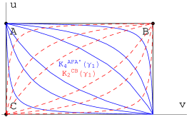
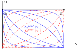
Figure 8: Families of kink orbits in each type of cell: a) $K_{2}^{AD}(\gamma_{1})$ and $K_{2}^{BC}(\gamma_{1})$ in Type 1 cells, b) $K_{2}^{BC}(\gamma_{1})$ and $K_{4}^{AA}(\gamma_{1})$ in Type 2 cells, and c) $K_{2}^{AA}(\gamma_{1})$ and $K_{2}^{BB}(\gamma_{1})$ in Type 3 cells.

Bearing this in mind, we shall describe the families of kink orbits inside the cells. In the cells where one or two of the foci are vertices that do not belong to ${\cal M}$ , kink orbits flowing according to (42) and connecting two elements of ${\cal M}$ are formed by gluing two families of solutions that correspond to two different choices of $\alpha$ relative to $\beta$. The gluing must be performed in such a way that the kink orbits back in the ${\mathbb{R}}^{2}$ Cartesian plane are continuous. We now describe the different types of kink orbits arising in different types of cells.

• In type 1 cells there are two families of kink orbits connecting opposite vertices in the cells, distinguished by ${\rm sign}((-1)^{\alpha+\beta})$ on (42). We shall refer to these two types respectively as $K_{2}^{AD}(\gamma_{1})$ when ${\rm sign}((-1)^{\alpha+\beta})=-1$, and $K_{2}^{CB}(\gamma_{1})$, if ${\rm sign}((-1)^{\alpha+\beta})=+1$. When ${\rm sign}((-1)^{\alpha+\beta})=-1$ $A$ is a stable node, and $D$ is an unstable node, or viceversa. In this case $B$ and $C$ are saddle points. If ${\rm sign}((-1)^{\alpha+\beta})=+1$ the pair of points $A$-$D$ exchanges its r$\hat{\rm o}$le with the $B$-$C$ couple, see Figure 8(a). The parameter $\gamma_{1}$ labels one member in each of the two families of kink orbits. The subscript suggests that these kinks are formed by two basic kinks/lumps, which can be confirmed by taking the asymptotic values: $\gamma_{1}\rightarrow\pm\infty$.

  To prove this last statement, we consider a solution characterized by the value $\gamma_{1}$. Therefore for generalized MSTB models (38) the orbit of this solution complies with:

  $$(-1)^{\alpha}\int\frac{du}{(u^{2}-\Omega^{2})u^{\alpha_{0}}\prod_{i=1}^{N}|u^{2}-\sigma_{i}^{2}|^{\alpha_{i}}}-(-1)^{\beta}\int\frac{dv}{(\Omega^{2}-v^{2})|v|^{\alpha_{0}}\prod_{i=1}^{N}|v^{2}-\sigma_{i}^{2}|^{\alpha_{i}}}=\sqrt{2}\gamma_{1}\quad.$$ (43)

  Linearization of (43) respectively near the point $C$ reads:

  $$\sqrt{2}\gamma_{1}=(-1)^{\alpha}\int\,du\,\frac{C_{u}(\sigma_{1},\dots,\sigma_{n+m})}{(u-\sigma_{k})^{\alpha_{k}}}-(-1)^{\beta}\int\,dv\,\frac{C_{v}(\sigma_{1},\dots,\sigma_{n+m})}{(v-\sigma_{j})^{\alpha_{j}}}\quad,$$ (44)

  where we have defined:

  $$C_{u}(\sigma_{1},\dots,\sigma_{n+m}) = \frac{1}{(\sigma_{k}^{2}-\Omega^{2})\sigma_{k}^{\alpha_{0}}\prod_{i=1}^{k-1}(\sigma_{k}^{2}-\sigma_{i}^{2})^{\alpha_{i}}(\sigma_{k+1}^{2}-\sigma_{k}^{2})^{\alpha_{k+1}}\prod_{i=k+2}^{n+m}(\sigma_{i}^{2}-\sigma_{k}^{2})^{\alpha_{i}}(2\sigma_{k})^{\alpha_{k}}}$$

  $$C_{v}(\sigma_{1},\dots,\sigma_{n+m}) = \frac{1}{(\Omega^{2}-\sigma_{j}^{2})\sigma_{j}^{\alpha_{0}}\prod_{i=1}^{j-1}(\sigma_{j}^{2}-\sigma_{i}^{2})^{\alpha_{i}}(\sigma_{j+1}^{2}-\sigma_{j}^{2})^{\alpha_{j+1}}\prod_{i=j+2}^{n+m}(\sigma_{i}^{2}-\sigma_{j}^{2})^{\alpha_{i}}(2\sigma_{j})^{\alpha_{j}}}$$

  Likewise, linearization of (43) respectively near the point $B$ reads:

  $$\sqrt{2}\gamma_{1} = (-1)^{\alpha}\int\,du\,\frac{B_{u}(\sigma_{1},\dots,\sigma_{n+m})}{(\sigma_{k+1}-u)^{\alpha_{k+1}}}-(-1)^{\beta}\int\,dv\,\frac{B_{v}(\sigma_{1},\dots,\sigma_{n+m})}{(\sigma_{j+1}-v)^{\alpha_{j+1}}}\,\,,$$ (45)

  where now we have

  $$B_{u}(\sigma_{1},\dots,\sigma_{n+m}) = \frac{1}{(\sigma_{k+1}^{2}-\Omega^{2})\sigma_{k+1}^{\alpha_{0}}\prod_{i=1}^{k-1}(\sigma_{k+1}^{2}-\sigma_{i}^{2})^{\alpha_{i}}(\sigma_{k+1}^{2}-\sigma_{k}^{2})^{\alpha_{k}}\prod_{i=k+2}^{n+m}(\sigma_{i}^{2}-\sigma_{k+1}^{2})^{\alpha_{i}}(2\sigma_{k+1})^{\alpha_{k+1}}}$$

  $$B_{v}(\sigma_{1},\dots,\sigma_{n+m}) = \frac{1}{(\Omega^{2}-\sigma_{j+1}^{2})\sigma_{j+1}^{\alpha_{0}}\prod_{i=1}^{j-1}(\sigma_{j+1}^{2}-\sigma_{i}^{2})^{\alpha_{i}}(\sigma_{j+1}^{2}-\sigma_{j}^{2})^{\alpha_{j}}\prod_{i=j+2}^{n+m}(\sigma_{i}^{2}-\sigma_{j+1}^{2})^{\alpha_{i}}(2\sigma_{j+1})^{\alpha_{j+1}}}\,\,.$$

  In (44) and (45), $C_{u}>0$, $C_{v}>0$, $B_{u}>0$,$B_{v}>0$ and the pertinent integrals are simple although we must distinguish between the cases $\alpha_{r}=1$ or $\alpha_{r}>1$ with $r=j,j+1,k,k+1$. Whichever the case, the limit $\gamma_{1}\rightarrow\infty$ in (44) and (45) provides us, for instance in the case $\alpha=\beta=1$, with the orbit $v=\sigma_{j}$ in (44), and $u=\sigma_{k+1}$ in (45), while the limit $\gamma_{1}\rightarrow-\infty$ yields the orbit $v=\sigma_{j+1}$ in (45) and $u=\sigma_{k}$ in (44). This means that the combination ${K}_{1}^{BD}+{K}_{1}^{DC}$ of singular kinks arises as $\gamma_{1}\rightarrow-\infty$ in the moduli space of $K_{2}^{BC}$ kinks while the combination ${\rm K}_{1}^{BA}+{K}_{1}^{AC}$ lives at the $\gamma_{1}=\infty$ boundary of the $K_{2}^{BC}$ kink moduli space. The same analysis can be tediously repeated in the rest of the cases. In sum, we find that:

  $$\lim_{|\gamma_{1}|\rightarrow\infty}K_{2}^{AD}(\gamma_{1})=\left\{\begin{array}[]{l}K_{1}^{AC}+K_{1}^{CD}\\ K_{1}^{AB}+K_{1}^{BD}\end{array}\right.\hskip 28.45274pt,\hskip 28.45274pt\lim_{|\gamma_{1}|\rightarrow\infty}K_{2}^{BC}(\gamma_{1})=\left\{\begin{array}[]{l}K_{1}^{BD}+K_{1}^{DC}\\ K_{1}^{BA}+K_{1}^{AC}\end{array}\right.\qquad.$$

  The $\gamma_{1}$ parameter, giving the orbit in the mechanical problem, measures the distance between the centers in the combination of basic kinks. Finite values of the parameter characterize the non-linear combinations of single kinks as the finite separation between lump centers. The kink families $K_{2}^{AD}(\gamma_{1})$ and $K_{2}^{CB}(\gamma_{1})$ are formed by different compositions of two kinks at different distances that become the basic or singular kinks when the inter-center distance is infinite.

• In type 2 cells there are also two families of kink orbits but one of the families is of a new type. If ${\rm sign}((-1)^{\alpha+\beta})=+1$, a $K_{2}^{BC}(\gamma_{1})$ family arises with identical properties to the $K_{2}^{BC}(\gamma_{1})$ family in type 1 cells. $B$ and $C$ are respectively stable and unstable nodes, or viceversa, and $A$ is a saddle point, see Figure 8(b).

  The novelty comes from the fact that in this type of cell, $D$ is a focus, $F$, that does not belong to ${\cal M}$ because it is not a fixed point of the trajectory flow. $F$ not being a fixed point, neither the $K_{2}^{AF}(\gamma_{1})$ nor the $K_{2}^{FA}(\gamma_{1})$ kink orbits -expected when ${\rm sign}((-1)^{\alpha+\beta})=-1$  and $A$ is either a stable or unstable node- can exist. In Figure 8(b) the apparent homoclinic kink trajectories $K_{4}^{AA}(\gamma_{1})$ are plotted in blue. These trajectories correspond to one $K_{2}^{AF}(\gamma_{1})$ and one $K_{2}^{FA}(\gamma_{1})$ kink orbit glued at the focus. One might think that such orbits fail to be derivable at the focus and consequently that their action is infinite, yielding field theoretical solutions of infinite energy. To examine this issue closely, it is convenient to go back to the Cartesian plane.

  Recall that the inverse map from ${\mathbb{E}}^{2}$ to ${\mathbb{R}}^{2}$ induced by the change to elliptic coordinates is one-to-two, see (20)): ${\mathbb{E}}^{2}$ is mapped into the upper half-plane $\phi_{2}>0$ by $\xi^{+*}$ and also into the lower half-plane $\phi_{2}<0$ by $\xi^{-*}$. Therefore, the inverse image of the point $A\equiv(\sigma_{n-1},\sigma_{n+1})$ is the two-element set: $A^{\pm}\equiv(\frac{\sigma_{n-1}\sigma_{n+1}}{\Omega},\pm\frac{\sqrt{(\sigma_{n+1}^{2}-\Omega^{2})(\Omega^{2}-\sigma_{n-1}^{2})}}{\Omega})$. The $K_{2}^{AF}(\gamma_{1})$ can be chosen to be mapped in the upper half-plane of the Cartesian plane ${\mathbb{R}}^{2}$ or viceversa. These two choices give rise to a family of continuous and derivable kink trajectories connecting the stable node $A^{+}$ with the unstable node $A^{-}$ (or viceversa when $A^{-}$ is stable and $A^{+}$ is unstable) . Therefore, every kink trajectory of this type is of finite energy, heteroclinic despite of appearing to be homoclinic in ${\mathbb{E}}^{2}$, and crosses from the upper half-plane to the lower half plane or viceversa through a single point: the focus $F$. The last point confirms that $F$ is a conjugate point to both $A^{+}$ and $A^{-}$ and, as anticipated, these trajectories are unstable according to the Morse index theorem. A laborious analysis, but conceptually identical to that shown for type 1 cells, shows that at the $|\gamma_{1}|\rightarrow\infty$ limit the following kink combination arises:

  $$\lim_{|\gamma_{1}|\rightarrow\infty}K_{4}^{AA}(\gamma_{1})=K_{1}^{AC}+K_{2}^{CF\bigvee FB}+K_{1}^{BA}\qquad\qquad,$$

  where by $K_{2}^{CF\bigvee FB}$ we denote the two-step singular kink orbit living respectively at the edges $u=\Omega$, and $v=\Omega$ in two different periods of time, the second period synchronized with the previous one at the focus $F\equiv(\Omega,\Omega)$. Note that

  $$K_{2}^{CF\bigvee FB}=\lim_{|\gamma_{1}|\rightarrow\infty}K_{2}^{CB}(\gamma_{1})$$

  and the two last limits above account for the subscript $4$ in the nomenclature. In ${\mathbb{R}}^{2}$, the $K_{2}^{CF\bigvee FB}$ kink orbit lives on the $\phi_{2}=0$ axis.

  The translation from this analysis in the analogous mechanical system to the field theory is as follows: 1) To this one-parametric family of finite-action heteroclinic kink orbits corresponds a one-parametric family of finite-energy topological kinks. 2) Because the kink orbits are unstable, the topological kinks are also unstable. 3) These kinks are composed of four basic kinks.

• In type 3 cells only two of the four vertices, $A\equiv(-\Omega,\sigma_{2})$, $B\equiv(\Omega,\sigma_{2})$, are elements of ${\cal M}$ whereas the other two vertices are the foci, $F_{\pm}\equiv(\pm\Omega,\Omega)$, of the elliptic coordinate system, that do not belong to ${\cal M}$. If ${\rm sign}((-1)^{\alpha+\beta})=+1$, $A$ is a stable or unstable node whereas $B$ is a saddle point. When ${\rm sign}((-1)^{\alpha+\beta})=-1$ the r$\hat{\rm o}$les of $A$ and $B$ are exchanged. Therefore, except for singular kink orbits all the generic kink trajectories cross one of the two foci, which are not fixed points but display indefinite flow.

  For these reasons, the features of the kink trajectories are better understood in the Cartesian plane. In ${\mathbb{R}}^{2}$ the vertices of the cell become: $A\equiv(-\sigma_{2},0)$, $B\equiv(\sigma_{2},0)$, and $F_{\pm}\equiv(\pm\Omega,0)$. Kink trajectories in the $K_{2}^{AA}(\gamma_{1})$ blue family start from $A$, run along the upper or the lower half-plane, meet at the $F_{+}$ focus, where they pass to the other half-plane, and come back to $B$. This tour is performed either clock- or counter-clockwise. The red kink trajectories in Figure 8(c) are identical to the blue kink trajectories of the same figure, but $B$ is the starting and ending point, and the bridge between half-planes is the $F_{-}$ focus. The kink orbits in type 3 cells are thus unstable homoclinic trajectories: each trajectory starts from either $A$ or $B$ and ends at either $A$ or $B$. The foci $F_{+}$ and $F_{-}$ are respectively conjugate points to $A$ and $B$ where all the members of the family meet. Again, it is hard but merely routine work to prove that the $|\gamma_{1}|=\infty$ limit is the following combination of singular kinks:

  $$\lim_{|\gamma_{1}|\rightarrow\infty}K_{2}^{AA}(\gamma_{1})=K_{1}^{AB}+{K}_{1}^{AF_{-}\bigvee F_{-}F_{+}\bigvee F_{+}B}\qquad\qquad,$$

  $$\lim_{|\gamma_{1}|\rightarrow\infty}K_{4}^{BB}(\gamma_{1})=K_{1}^{BA}+{K}_{1}^{BF_{+}\bigvee F_{+}F_{-}\bigvee F_{-}A}\qquad\qquad.$$

  ${K}_{1}^{AF_{-}\bigvee F_{-}F_{+}\bigvee F_{+}B}$ denotes the three-step singular kink orbit living respectively at the edges $v=-\Omega$, $u=\Omega$, and $v=\Omega$ in three different periods of time, the second period synchronized with the previous and later periods at the foci. Until now we have met only kinks for which the number of the steps coincides with the number of lumps. For instance, the kink orbit $K_{2}^{CF\bigvee FB}$ runs over two edges, and even though the energy density of these stable kinks is formed by a single lump, it is exactly the superposition of one $K_{1}^{AC}$ and one $K_{1}^{CB}$ kinks with coinciding centers. ${K}_{1}^{AF_{-}\bigvee F_{-}F_{+}\bigvee F_{+}B}$ kinks differ in two ways: 1) Combinations of three $K_{1}^{AB}$ do not form these kinks. 2) ${K}_{1}^{AF_{-}\bigvee F_{-}F_{+}\bigvee F_{+}B}$ kinks are unstable because upon crossing one of the two foci they pass a conjugate point of the congruence of kink orbits they belong to. In sum, there are no reasons for this configuration to be considered as a composite kink and, moreover, ${K}_{1}^{AF_{-}\bigvee F_{-}F_{+}\bigvee F_{+}B}$ kinks are unstable.

  The translation from this analysis in the analogous mechanical system to the field theory is as follows: 1) To this one-parametric family of finite action homoclinic kink orbits corresponds a one-parametric family of finite energy non-topological kinks. 2) Because the kink orbits are unstable the non-topological kinks are unstable. 3) These kinks are composed of one basic kink and one unstable singular kink, see [32].

The previous results can be summarized as follows:

Proposition 3. There are families of kink orbits confined in each cell in the elliptic plane. The kink trajectories connect elements of ${\cal M}$ at opposite cell vertices. We shall denote these generic kink orbits by labelling the vertices connected by them: $K_{2}^{AD}(\gamma_{1})$, $K_{2}^{BC}(\gamma_{1})$. There are two special cases: either one or two cell vertices are not zeroes of $V(\phi_{1},\phi_{2})$. In type I-1a and type I-1b generalized MSTB models type 2 cells arise: in these cells there is a family of topological kink orbits connecting the elements $A^{+}=\xi^{+}(\sigma_{n-1},\sigma_{n+1})$ and $A^{-}=\xi^{-}(\sigma_{n-1},\sigma_{n+1})$ of ${\cal M}$ in ${\mathbb{R}}^{2}$; every orbit in this family passes through one of the two foci. In $n=1$ type I-1a generalized MSTB models there is one cell of type 3; in this cell there is a family of non-topological kink orbits joining the points $A=(-\Omega,\sigma_{2})$ or $B=(\Omega,\sigma_{2})$ with themselves. Each non-topological kink orbit crosses one of the two $F_{\pm}$ foci.

3.3 Sum rules of kink masses

The action of the mechanical trajectory is the energy of the static field profile. Therefore,

$${E}[(\phi_{1},\phi_{2}] = \int_{\xi^{*}\phi}du\,\,{\rm sign}({u}^{\prime})\sqrt{\frac{2(F+Eu^{2}+f(u))}{u^{2}-\Omega^{2}}}+$$

$$+ \int_{\xi^{*}\phi}dv\,\,{\rm sign}({v}^{\prime})\sqrt{\frac{2(-F-Ev^{2}+g(v))}{\Omega^{2}-v^{2}}}-\left.Ex\right|_{\xi^{*}\phi}\qquad,$$

which is the Hamilton principal function -the action- of the mechanical trajectories, is also the energy of the static field solutions. Solitary wave solutions have finite energy $E[\phi_{1},\phi_{2}]$ and correspond to trajectories with zero mechanical energy and zero separation constant: $E=F=0$.

Proposition 4. The energy of the kinks in generalized MSTB models is the mechanical action of the kink orbits:

$${E}[\phi_{1},\phi_{2}]=\left|\int_{\pi_{u}(\xi^{*}\vec{\phi})}du\hskip 5.69046pt\sqrt{\frac{2f(u)}{u^{2}-\Omega^{2}}}\right|+\left|\int_{\pi_{v}(\xi^{*}\vec{\phi})}dv\hskip 5.69046pt\sqrt{\frac{2g(v)}{\Omega^{2}-v^{2}}}\right|\qquad,$$ (46)

where $\pi_{u}(\xi^{*}\vec{\phi})$ and $\pi_{v}(\xi^{*}\vec{\phi})$ are respectively the projections of the point $\xi^{*}\vec{\phi}$ of the kink orbit into the axes $u$ and $v$.

Therefore, all the members of the kink family are iso-energetic. Formula (46) allows us to state the following:

1. The kink energy does not depend on the fine details of the solitary waves: kinks with very different profiles share the same energy. The kink energy is determined only by the projections of the kink trajectories into the axes.

2. The important implication of this is that the energy of any member of a family of composite kinks is uniquely determined as the sum of the energies of the basic or singular kinks. The total energy of the singular kinks is:

   $${E}[K_{1}^{AB}]={E}[K_{1}^{CD}]=\left|\int_{\sigma_{j}}^{\sigma_{j+1}}dv\hskip 2.84544pt\sqrt{\frac{2g(v)}{\Omega^{2}-v^{2}}}\,\right|;\hskip 8.5359pt{E}[K_{1}^{AC}]={E}[K_{1}^{BD}]=\left|\int_{\sigma_{k}}^{\sigma_{k+1}}du\hskip 2.84544pt\sqrt{\frac{2f(u)}{u^{2}-\Omega^{2}}}\,\right|$$ (47)

   A little more care is needed when the foci are crossed by a congruence of kink trajectories. Here, line integrals must be computed piecewise: from the starting point to the focus and from the focus to the endpoint. For instance, the energy of ${\rm K}_{2}^{CF\bigvee FB}$ kinks in Type I-1a and I-1b generalized MSTB models is:

   $${E}[K_{2}^{CF\bigvee FB}]=\left|\int_{\sigma_{n-1}}^{\Omega}dv\hskip 2.84544pt\sqrt{\frac{2g(v)}{\Omega^{2}-v^{2}}}\,\right|+\left|\int_{\Omega}^{\sigma_{n+1}}du\hskip 2.84544pt\sqrt{\frac{2f(u)}{u^{2}-\Omega^{2}}}\,\right|\qquad.$$ (48)

   Simili modo, the energy of unstable singular kinks ${K}_{1}^{AF_{-}\bigvee F_{-}F_{+}\bigvee F_{+}A}$ in type 3 cells of $n=1$ Type I-1a generalized MSTB models is also computed piecewise:

   $$E[{K}_{1}^{AF_{-}\bigvee F_{-}F_{+}\bigvee F_{+}B}]=\left|\int_{-\Omega}^{\Omega}dv\hskip 2.84544pt\sqrt{\frac{2g(v)}{\Omega^{2}-v^{2}}}\,\right|+2\left|\int_{\Omega}^{\sigma_{2}}du\hskip 2.84544pt\sqrt{\frac{2f(u)}{u^{2}-\Omega^{2}}}\,\right|\qquad.$$ (49)

3. Kinks or combinations of kinks that have the same projections on the elliptic axes have the same energy. This is the crux of the matter of the kink mass sum rules. We now write all the kink mass sum rules observed in the generalized MSTB models. These sum rules connect the energy of the kinks solutions confined in a cell, and hence we must distinguish three possible cases:

   $$\bullet$$ Kinks confined in cells of Type 1:

   $$\hskip 19.91684ptE[K_{1}^{AB}]=E[K_{1}^{CD}]\hskip 14.22636pt;\hskip 14.22636ptE[K_{1}^{AC}]=E[K_{1}^{BD}]$$

   $$\hskip 19.91684ptE[K_{2}^{AD}(\gamma_{1})]=E[K_{2}^{BC}(\gamma_{1})]=E[K_{1}^{AB}]+E[K_{1}^{AC}]$$

   $$\bullet$$ Kinks confined in cells of Type 2:

   $$\hskip 19.91684ptE[K_{2}^{CF\bigvee FB}]=E[K_{1}^{AB}]+E[K_{1}^{AC}]=E[K_{2}^{CB}(\gamma_{1})]$$

   $$\hskip 19.91684ptE[K_{4}^{AA}(\gamma_{1})]=2E[K_{1}^{AB}]+2E[K_{1}^{AC}]$$

   $$\bullet$$ Kinks confined in cells of Type 3:

   $$\hskip 19.91684ptE[K_{2}^{AA}(\gamma_{1})]=E[K_{1}^{AB}]+E[{K}_{1}^{AF_{-}\bigvee F_{-}F_{+}\bigvee F_{+}B}]=E_{2}^{BB}(\gamma_{1})$$

   $$\hskip 19.91684ptE_{2}^{BB}(\gamma_{1})=E[K_{1}^{BA}]+E[{K}_{1}^{BF_{+}\bigvee F_{+}F_{-}\bigvee F_{-}A}]$$

   These kink mass sum rules are due to the Hamilton-Jacobi separability in elliptic coordinates of the mechanical systems ruling finite energy static solutions in the generalized MSTB models.

3.4 Kink orbits as gradient flow lines

It is interesting to address the results of the previous sub-Section from the point of view sketched in the Introduction. The Bogomolny’i-Prasad-Sommerfield understanding of several types of topological defects in field theory, such as kinks, special classes of vortices and magnetic monopoles, and instantons, can be applied to some solitary waves of generalized MSTB models. We recall that the BPS approach is possible if the potential energy density is equal to half the norm of the square of the norm of a function $W(\phi_{1},\phi_{2})$, see (2):

$$U(\phi_{1},\phi_{2})={1\over 2}\left(\frac{\partial W}{\partial\phi_{1}}\cdot\,\frac{\partial W}{\partial\phi_{1}}+\frac{\partial W}{\partial\phi_{2}}\cdot\,\frac{\partial W}{\partial\phi_{2}}\right)={1\over 2}\vec{\nabla}W\cdot\vec{\nabla}W\qquad.$$ (50)

Writing the static energy in the form (3)

$$E[\vec{\phi}]=\frac{1}{2}\int dx\left[\frac{d\vec{\phi}}{dx}-\vec{\nabla}W\right]\cdot\left[\frac{d\vec{\phi}}{dx}-\vec{\nabla}W\right]+\int dW\qquad.$$ (51)

one sees that solutions of the first-order ODE system

$$\frac{\vec{d\phi}}{dx}=\vec{\nabla}W(\phi_{1},\phi_{2})=\frac{\partial W}{\partial\phi_{1}}\vec{e}_{1}+\frac{\partial W}{\partial\phi_{2}}\vec{e}_{2}$$ (52)

are absolute minima of the energy if $W$ behaves well enough. Stable kink orbits are thus the flow lines induced by the gradient of $W$, usually referred to as the superpotential in physicists’ literature, because of the central r$\hat{\rm o}$le that this function plays in supersymmetric models. A closer look to (50) reveals that $W$ is no more than a solution of the time-independent Hamilton-Jacobi equation of the analogous mechanical system with zero mechanical energy: i.e., the superpotential is the $E=0$ Hamilton characteristic function in Hamiltonian dynamical systems.

For mechanical potential energies of Liouville Type I systems, (50) in elliptic coordinates reads:

$$\frac{1}{2(u^{2}-v^{2})}\left\{(u^{2}-\Omega^{2})\left(\frac{\partial W}{\partial u}\right)^{2}+(\Omega^{2}-v^{2})\left(\frac{\partial W}{\partial v}\right)^{2}\right\}=\frac{1}{u^{2}-v^{2}}\left(f(u)+g(v)\right)\qquad.$$ (53)

The separation ansatz $W(u,v)=W_{1}(u)+W_{2}(v)$ reduces the PDE (53) to two independent first-order differential equations

$$\frac{dW_{1}}{du}=(-1)^{\alpha}\sqrt{\frac{2f(u)}{u^{2}-\Omega^{2}}}\hskip 56.9055pt\frac{dW_{2}}{dv}=(-1)^{\beta}\sqrt{\frac{2g(v)}{\Omega^{2}-v^{2}}}\qquad,$$

which can be integrated by quadratures:

$$W^{(\alpha,\beta)}(u,v)=(-1)^{\alpha}\int du\sqrt{\frac{2f(u)}{u^{2}-\Omega^{2}}}+(-1)^{\beta}\int dv\sqrt{\frac{2g(v)}{\Omega^{2}-v^{2}}}\qquad,\qquad\alpha,\beta=0,1\qquad.$$ (54)

Proposition 5: Generalized MSTB models are built from the complete integral -(54)- of the time-independent Hamilton-Jacobi equation with zero mechanical energy for the analogous mechanical system. In modern language, we characterize the generalized MSTB model as those admitting four different superpotentials according to the freedom of choice of signs in (54).

More precisely,

Proposition 6: In ${\mathbb{E}}^{2}$ the four superpotentials of generalized MSTB models have the form:

$$\xi_{\Omega}^{*}W=W_{1}(u)+W_{2}(v)\hskip 28.45274pt\equiv\hskip 28.45274pt\frac{\partial^{2}(\xi_{\Omega}^{*}W)}{\partial u\,\partial v}=0\qquad.$$ (55)

In ${\mathbb{R}}^{2}$ the PDE (55) becomes the cumbersome PDE satisfied by generalized MSTB superpotentials:

$$\phi_{1}\phi_{2}\left(\frac{\partial^{2}W}{\partial\phi_{1}\partial\phi_{1}}-\frac{\partial^{2}W}{\partial\phi_{2}\partial\phi_{2}}\right)+(\phi_{2}\phi_{2}-\phi_{1}\phi_{1}+\Omega^{2})\frac{\partial^{2}W}{\partial\phi_{1}\partial\phi_{2}}+\phi_{2}\frac{\partial W}{\partial\phi_{1}}-\phi_{1}\frac{\partial W}{\partial\phi_{2}}=0\qquad.$$ (56)

The concept of superpotential allows us to write the invariants (16) of the mechanical system in the surprisingly simpler form:

$$I_{1} = \frac{1}{2}\left(\frac{d\phi_{1}}{dx}\right)^{2}+\frac{1}{2}\left(\frac{d\phi_{2}}{dx}\right)^{2}-\frac{1}{2}\left(\frac{\partial W}{\partial\phi_{1}}\right)^{2}-\frac{1}{2}\left(\frac{\partial W}{\partial\phi_{2}}\right)^{2}$$ (57)

$$I_{2} = \frac{1}{2}\left[\left(\phi_{2}\frac{d\phi_{1}}{dx}-\phi_{1}\frac{d\phi_{2}}{dx}\right)^{2}-\Omega^{2}\frac{d\phi_{2}}{dx}\frac{d\phi_{2}}{dx}-\left(\phi_{2}\frac{\partial W}{\partial\phi_{1}}-\phi_{1}\frac{\partial W}{\partial\phi_{2}}\right)^{2}+\Omega^{2}\frac{\partial W}{\partial\phi_{2}}\frac{\partial W}{\partial\phi_{2}}\right]\quad,$$ (58)

explicitly showing that $I_{1}=0=I_{2}$ for the solutions of (52).

Obviously, because four superpotentials are available there are four different ways of saturating the BPS bound [8]. For instance, in ${\mathbb{E}}^{2}$ these equations are:

$$\frac{du}{dx}=(-1)^{\alpha}\frac{\sqrt{2(u^{2}-\Omega^{2})f(u)}}{u^{2}-v^{2}}\hskip 28.45274pt,\hskip 28.45274pt\frac{dv}{dx}=(-1)^{\beta}\frac{\sqrt{2(\Omega^{2}-v^{2})g(v)}}{u^{2}-v^{2}}\qquad.$$ (59)

It is clear that for kink orbit solutions of (54) the kink energy

$$E[\vec{\phi}_{K}]=\int_{K}\,dW\qquad\qquad,$$

the integral of the exterior derivative of the superpotential along the kink trajectories, is precisely given by formulas (46), (47), (48), and (49) for the different types of kinks. If the kink orbit does not cross points where $W$ is not differentiable Stoke’s theorem rules that

$$E[\vec{\phi}_{K}]=\left|W(\vec{\phi}_{I})-W(\vec{\phi}_{J})\right|\qquad\quad,$$

and the energy of stable kinks is a topological charge. The situation is more subtle for kink orbits that cross non-fixed conjugate points. Stoke’s theorem must be applied piece-wise, and we find:

$$E[\vec{\phi}_{K}]=\left|W(\vec{\phi}_{I})-W(\mp\Omega\vec{e}_{1}))\right|+\left|W(\mp\Omega\vec{e}_{1})-W(\vec{\phi}_{J})\right|\qquad,\qquad E[\vec{\phi}_{K}]=2\left|W(\vec{\phi}_{I})-W(\mp\Omega\vec{e}_{1})\right|\,\,\,,$$

respectively for unstable kink orbits in Type 2 and Type 3 cells. The important point is that these kink orbits are not solutions of (59) for the same choice of $\alpha$ and $\beta$ over the whole real line ${\mathbb{R}}$. The unstable trajectories solve (54) for a given $\beta$ relative to $\alpha$ between $x=-\infty$ and $x=x_{0}$, the point where the focus is reached. Between $x_{0}$ and $x=+\infty$, the first-order equations satisfied correspond to the other relation between $\beta$ and $\alpha$. The unstable kink orbits, however, satisfies the static second-order equations (16) but the unstable kinks do not saturate the BPS bound.

We show explicitly that the existence of four superpotentials is connected to the Hamilton-Jacobi separability of the analogous mechanical system to generalized MSTB models in elliptic coordinates. Formulas (26) and (27) for the two invariants in elliptic coordinates due to HJ separability provide the following identities for the square of $u$ and $v$ derivatives:

$$\left(\frac{du}{dx}\right)^{2} = \frac{2(u^{2}-\Omega^{2})\left[-I_{2}+I_{1}(u^{2}-\Omega^{2})+f(u)\right]}{(u^{2}-v^{2})^{2}}$$

$$\left(\frac{dv}{dx}\right)^{2} = \frac{2(\Omega^{2}-v^{2})\left[I_{2}+I_{1}(\Omega^{2}-v^{2})+g(v)\right]}{(u^{2}-v^{2})^{2}}\qquad.$$

The separatrix trajectories between bound and unbound motion arise for $I_{1}=0$, $I_{2}=0$, values for which the above equations reduce to:

$$\left(\frac{du}{dx}\right)^{2}=\frac{2f(u)(u^{2}-\Omega^{2})}{(u^{2}-v^{2})^{2}}\hskip 28.45274pt,\hskip 28.45274pt\left(\frac{dv}{dx}\right)^{2}=\frac{2g(v)(\Omega^{2}-v^{2})}{(u^{2}-v^{2})^{2}}\qquad,$$ (60)

equivalent to (59) with the four sign combinations. Complete Arnold-Liouville integrability is accompanied by HJ separability, allowing us to obtain all the separatrix trajectories - all the kink profiles- from the complete solution of the HJ equation: the four superpotentials. The partial solvability of the HJ equation would permit only a partial identification of the kink manifold. The complete solution of the HJ equation for arbitrary values (non-zero) of the invariants,

$$W^{(\alpha,\beta)}=(-1)^{\alpha}\int du\sqrt{\frac{2(-I_{2}+I_{1}(u^{2}-\Omega^{2})+f(u))}{u^{2}-\Omega^{2}}}\,\,+(-1)^{\beta}\int du\sqrt{\frac{2(I_{2}+I_{1}(\Omega^{2}-v^{2})+g(v))}{\Omega^{2}-v^{2}}}$$

also reduces to algebraic equations between quadratures all the other trajectories - either periodic or unbounded- of the analogous mechanical system. Back in field theory, the periodic orbits are interpreted as (unstable) kinks on a circle (the space-time being ${\mathbb{R}}\times{\mathbb{S}}^{1}$ with hyperbolic metric) whereas unbound mechanical motion corresponds to static field solutions of infinite energy.

To finish this Section and a thorough study of generalized MSTB models we now address this issue in ${\mathbb{R}}^{2}$, i.e., we analyze the $I_{1}=0=I_{2}$ condition in Cartesian coordinates. The surprise is that not only it is satisfied by solutions of the first-order ODE system (52), but that solutions of the new first-order ODE system

$$\frac{d\phi_{1}}{dx} = \mp\frac{(\Omega^{2}-\phi_{1}^{2}+\phi_{2}^{2})\frac{\partial W}{\partial\phi_{1}}-2\phi_{1}\phi_{2}\frac{\partial W}{\partial\phi_{2}}}{\sqrt{[(\phi_{1}-\Omega)^{2}+\phi_{1}^{2}][(\phi_{1}+\Omega)^{2}+\phi_{2}^{2}]}}$$

$$\frac{d\phi_{2}}{dx} = \pm\frac{(\Omega^{2}-\phi_{1}^{2}+\phi_{2}^{2})\frac{\partial W}{\partial\phi_{2}}+2\phi_{1}\phi_{2}\frac{\partial W}{\partial\phi_{1}}}{\sqrt{[(\phi_{1}-\Omega)^{2}+\phi_{1}^{2}][(\phi_{1}+\Omega)^{2}+\phi_{2}^{2}]}}$$ (61)

also comply with $I_{1}=0=I_{2}$!. This implies the existence of a second superpotential $\tilde{W}$. The vector field from the right hand sides of (61):

$$\vec{A}(\phi_{1},\phi_{2})=\mp\left[\frac{(\Omega^{2}-\phi_{1}^{2}+\phi_{2}^{2})\frac{\partial W}{\partial\phi_{1}}-2\phi_{1}\phi_{2}\frac{\partial W}{\partial\phi_{2}}}{\sqrt{[(\phi_{1}-\Omega)^{2}+\phi_{1}^{2}][(\phi_{1}+\Omega)^{2}+\phi_{2}^{2}]}}\vec{e}_{1}-\frac{(\Omega^{2}-\phi_{1}^{2}+\phi_{2}^{2})\frac{\partial W}{\partial\phi_{2}}+2\phi_{1}\phi_{2}\frac{\partial W}{\partial\phi_{1}}}{\sqrt{[(\phi_{1}-\Omega)^{2}+\phi_{1}^{2}][(\phi_{1}+\Omega)^{2}+\phi_{2}^{2}]}}\vec{e}_{2}\right]\quad,$$

despite its horrible aspect, is curl-less because equation (56) is valid in Type I Liouville models. Therefore, Green’s theorem ensures that there exists a function $\tilde{W}$ such that (61) is equivalent to the first-order ODE system: $\frac{d\phi_{1}}{dx}=\frac{\partial\tilde{W}}{\partial\phi_{1}}$, $\frac{d\phi_{2}}{dx}=\frac{\partial\tilde{W}}{\partial\phi_{2}}$. Four different superpotentials, $\pm W$, $\pm\tilde{W}$, are also available in Cartesian coordinates.

4 Eighth-order generalized MSTB models

The general analysis of the previous Section affords us a practical method of obtaining the kink variety of generalized MSTB models by means of a few computations. The references [16-28] are devoted to the original MSTB model, in which the potential energy density is a quartic polynomial in the two scalar fields. In the paradigm of generalized MSTB models, the functions $f$ and $g$ are respectively: $f(u)=\frac{1}{2}(u^{2}-1)^{2}(u^{2}-\Omega^{2})$ and $g(v)=\frac{1}{2}(v^{2}-1)^{2}(\Omega^{2}-v^{2})$. Therefore, $\bar{\cal M}_{g}=\{\sigma_{-1}=-\Omega;\sigma_{1}=\Omega\}$ and $\bar{\cal M}_{f}=\{\sigma_{1}=\Omega;\sigma_{2}=1\}$ such that $m=1$ and $n=1$, a type I-1a generalized MSTB model that involves only the type 3 cell $C_{-11}^{12}$ in the reticulum $\cal{R}$. There are only two singular kinks: $K_{1}^{AB}$ and ${K}_{1}^{AF_{-}\bigvee F_{-}F_{+}\bigvee F_{+}B}$ (respectively denoted as TK2 and TK1 kinks in the literature). The remaining kinks form a family of non-topological (unstable) kinks: $K_{2}^{AA}$ (usually referred to as NTK2 kinks). In other papers, [29-31], a generalized MSTB model where the potential energy density is a degree-six polynomial in the fields is discussed. The $f$ and $g$ functions in this model are: $f(u)=\frac{1}{2}u^{2}(u^{2}-1)^{2}(u^{2}-\sigma^{2})$ and $g(v)=\frac{1}{2}v^{2}(v^{2}-1)^{2}(\sigma^{2}-v^{2})$. A type I-1b generalized MSTB model with $m=1$ and $n=1$ arises. The set of zeroes of $g$ and $f$ are respectively $\bar{\cal M}_{g}=\{\sigma_{-1}=-\Omega;\sigma_{0}=0;\sigma_{1}=\Omega\}$ and $\bar{\cal M}_{f}=\{\sigma_{1}=\Omega;\sigma_{2}=1\}$ whereas the set of minima of the potential in ${\mathbb{R}}^{2}$ is, using the notation of [37], ${\cal M}=\{A_{\pm}=(\pm 1,0);B_{\pm}=(0,\pm\sqrt{1-\sigma^{2}});O=(0,0)\}$. The reticulum in ${\mathbb{R}}^{2}$ is formed by two type 2 cells joined by the edge on the ordinate axis. There are three singular kinks, denoted as $K_{1}^{AO}$, $K_{1}^{BO}$ and $K_{1}^{AB}$, and two families of topological composite kinks, one of them stable, $K_{2}^{AO}(\gamma_{1})$, and the other one, $K_{2}^{BB}(\gamma_{1})$, unstable.

To close this article we shall study a two-parametric family of generalized MSTB models with an eight-order polynomial as potential energy density:

$$U(\phi_{1},\phi_{2})=(\phi_{1}^{2}+\phi_{2}^{2}-\sigma^{2})^{2}(\phi_{1}^{2}+\phi_{2}^{2}-\tau^{2})^{2}+3\Omega^{2}\phi_{2}^{2}\left(\phi_{1}^{2}+\phi_{2}^{2}+\textstyle\frac{\Omega^{2}-2\sigma^{2}-2\tau^{2}}{3}\right)^{2}+\alpha\phi_{2}^{2}+\Omega^{2}\tau^{2}\phi_{2}^{4}$$ (62)

where $\alpha=\frac{\Omega^{2}}{3}(2\Omega^{4}-2\sigma^{2}\Omega^{2}-2\tau^{2}\Omega^{2}+4\Omega^{2}-\sigma^{4}-\tau^{4})$ and $\Omega^{2}=\sigma^{2}\tau^{2}$.

         

Figure 9: Potential density energy in the model ($\tau<\sigma<1$) and bifurcation of the elements of ${\cal M}$.

The parameters $\sigma$ and $\tau$ are the coupling constants of these generalized MSTB models and the foci of the elliptic coordinate system are determined from their product. The four superpotentials are:

$$W(\phi_{1},\phi_{2}) = \pm\frac{\sqrt{2}}{12}\sqrt{(\phi_{1}\pm\Omega)^{2}+\phi_{2}^{2}}\left[3(\phi_{1}^{2}+\phi_{2}^{2}\mp\Omega\phi_{1}+\Omega^{2})(\phi_{1}^{2}+\phi_{2}^{2}\pm\Omega\phi_{1}+\Omega^{2})-\right.$$ (63)

$$\left.-5(\sigma^{2}+\tau^{2})(\phi_{1}^{2}+\phi_{2}^{2}\mp\Omega\phi_{1}+\Omega^{2})\mp 3\Omega\phi_{1}(\phi_{1}^{2}+\phi_{2}^{2}+\Omega^{2})+15\Omega^{2}\right]\qquad.$$

The secret to finding a complete solution to the zero mechanical energy Hamilton-Jacobi equation of the analogous mechanical system is that the mechanical system is of Stackel type. There are two invariants in involution -the mechanical energy, $I_{1}$, and a generalized momentum, $I_{2}$- that are quadratic in the momenta:

$$I_{1} = \frac{1}{2}\left(\frac{d\phi_{1}}{dx}\right)^{2}+\frac{1}{2}\left(\frac{d\phi_{2}}{dx}\right)^{2}-U(\phi_{1},\phi_{2})$$ (64)

$$I_{2} = \frac{1}{2}\left(\phi_{1}\frac{d\phi_{2}}{dx}-\phi_{2}\frac{d\phi_{1}}{dx}\right)^{2}-\frac{\Omega^{2}}{2}\left(\frac{d\phi_{2}}{dx}\right)^{2}-\Omega^{2}\phi_{2}^{2}(\phi_{1}^{2}+\phi_{2}^{2}+\delta)\left[(\phi_{1}^{2}+\phi_{2}^{2}-\kappa)^{2}+2\Omega^{2}\phi_{2}^{2}+\beta\right]\,.$$ (65)

The mechanical system is amenable to the separation of variables. Here, $\beta=\Omega^{2}(\Omega^{2}-\sigma^{2}-\tau^{2}+\frac{3}{2})-\frac{1}{4}(\sigma^{4}+\tau^{4})$, $\delta=\Omega^{2}-\sigma^{2}-\tau^{2}$ and $\kappa=\frac{\sigma^{2}+\tau^{2}}{2}$.

In the count and localization of the elements of ${\cal M}$ a complicated process of bifurcation arises, depending on the values of the parameters $\tau$ and $\sigma$. To analyze the most interesting cases, we shall consider a fixed value of $\sigma\in(0,1)$ and let allow $\tau$ to vary along the real line. If both parameters are greater than or equal to one the model presents only isolated singular kinks. There are three cases - 1) $\tau<1$; 2) $\tau=1$, and 3) $\tau>1$- where degenerate kink families arise in the model. In Figure 9b we show the elements of ${\cal M}$ when $\tau$ is varied from 0 to 3. If $\tau\in(0,1)$, ${\cal M}$ is formed by four elements living at the intersection points of the two enveloping ellipses of the separatrix trajectories with the $\phi_{1}$-axis. For $\tau>1$ there are still four elements of ${\cal M}$ in the $\phi_{1}$-axis but also another four elements of ${\cal M}$ at the intersection of the enveloping ellipse and hyperbola of the separatrix trajectories arise. $\tau=1$ marks a pitchfork bifurcation of the elements in the interior ellipse when this curve becomes a hyperbola for $\tau>1$ . All these statements become clear looking at the potential energy density in elliptic variables:

$$\xi_{\sigma\tau}^{*}U(\phi_{1},\phi_{2})=\frac{1}{u^{2}-v^{2}}\left[(u^{2}-\sigma^{2})^{2}(u^{2}-\tau^{2})^{2}(u^{2}-\Omega^{2})+(v^{2}-\sigma^{2})^{2}(v^{2}-\tau^{2})^{2}(\Omega^{2}-v^{2})\right]$$ (66)

Comparison between (66) and (28) shows that we are dealing with a family of generalized MSTB models.

4.1 The structure of the set ${\cal M}$

We shall now describe the distribution of the zeroes of the potential energy density both in ${\mathbb{E}}^{2}$ and ${\mathbb{R}}^{2}$ successively for $\tau<1$, $\tau>1$, and $\tau=1$.

• Regime I: $0<\tau^{2}<\sigma^{2}<1$. The model belongs to type I-1a generalized MSTB models. Because $\Omega<\tau<\sigma$ we have: $n=1$ , $m=2$. The set of roots of $g$ and $f$ are respectively $\bar{\cal M}_{g}=\{\sigma_{-1}=-\Omega;\sigma_{1}=\Omega\}$ and $\bar{\cal M}_{f}=\{\sigma_{1}=\Omega;\sigma_{2}=\tau;\sigma_{3}=\sigma\}$. Therefore, the set of zeroes of $U(\phi_{1},\phi_{2})$ has four elements, both in ${\mathbb{E}}^{2}$ and ${\mathbb{R}}^{2}$, in this range of the parameters:

  $$\bar{\cal M}_{\rm I}=\{\bar{A}_{\pm}=(\sigma,\pm\Omega);\bar{B}_{\pm}=(\tau,\pm\Omega)\}\qquad,\qquad{\cal M}_{\rm I}=\{A_{\pm}=(\pm\sigma,0);B_{\pm}=(\pm\tau,0)\}\quad.$$

  The model exhibits symmetry with respect to the Klein four-group ${\mathbb{Z}}_{2}^{2}$ generated by the reflections of the fields: $\phi_{1}\rightarrow-\phi_{1}$ and $\phi_{2}\rightarrow-\phi_{2}$. In the quantum version of the model, the symmetry with respect to the ${\mathbb{Z}}^{2}$ sub-group generated by $\phi_{1}\rightarrow-\phi_{1}$, however, is broken by the choice of any $A$ or $B$ ground state. The set ${\cal M}_{\rm I}$ is formed by the $A$- and $B$-orbits of this sub-group, such that the moduli space of vacua has two elements: ${\cal M}_{\rm I}/{\mathbb{Z}}_{2}^{2}=\{A,B\}$.

  In Figure 10 the reticulum corresponding to this regime is shown. It is formed by two cells: $C_{-11}^{12}$, a type 3 cell delimited by the edges $B_{+}B_{-}$, $B_{+}F_{+}$, $F_{+}F_{-}$, $F_{-}B_{-}$, and $C_{-11}^{23}$, a type 1 cell whose vertices are the points $A_{+}$, $A_{-}$, $B_{+}$, and $B_{-}$. On the Cartesian plane, ${\mathbb{R}}^{2}$, the cell $C_{-11}^{23}$ is the region confined between the two ellipses

  $$\phi_{1}^{2}+\frac{\phi_{2}^{2}}{\bar{\sigma}^{2}}=\tau^{2}\qquad({\rm left})\qquad,\qquad\qquad\phi_{1}^{2}+\frac{\phi_{2}^{2}}{\bar{\tau}^{2}}=\sigma^{2}\qquad({\rm right})\qquad,$$ (67)

  whereas $C_{-11}^{12}$ is the region bounded by the ellipse (67)(right). To simplify this and subsequent formulas we use the following conventions: $\bar{\sigma}=\sqrt{1-\sigma^{2}}$, $\bar{\tau}=\sqrt{|1-\tau^{2}|}$.

  

  Figure 10: Reticulum in ${\mathbb{E}}^{2}$ and elements of $\bar{\cal M}$ in the regime I. Image in ${\mathbb{R}}^{2}$.

• Regime II: $0<\sigma^{2}<1<\tau^{2}$. Because $\sigma<\Omega<\tau$, the model also belongs to Type I 1a generalized MSTB models in this regime, but now: $n=2$, $m=1$. The set of roots of $g$ and $f$ are respectively: $\bar{\cal M}_{g}=\{\sigma_{-2}=-\Omega;\sigma_{-1}=-\sigma;\sigma_{1}=\sigma;\sigma_{2}=\Omega\}$, $\bar{\cal M}_{f}=\{\sigma_{2}=\Omega;\sigma_{3}=\tau\}$. The cardinal of the set of zeroes of the potential energy in the elliptic strip ${\mathbb{E}}^{2}$ differs from the same number in the Cartesian plane ${\mathbb{R}}^{2}$. $\bar{\cal M}_{\rm II}$ has six elements whereas ${\cal M}_{\rm II}$ contains eight:

  $$\bar{\cal M}_{\rm II}=\{\bar{A}_{\pm}=(\tau,\pm\Omega)\,;\,\bar{B}_{\pm}=(\Omega,\pm\sigma)\,;\,C_{\pm}^{\pm}=(\tau,\pm\sigma)\,\}$$

  $${\cal M}_{\rm II}=\{A_{\pm}=(\pm\tau,0)\,;\,B_{\pm}=(\pm\sigma,0)\,;\,C_{\pm}^{+}=(1,\pm\bar{\Omega})\,;\,C_{\pm}^{-}=(-1,\pm\bar{\Omega})\}\quad,\quad\bar{\Omega}=\bar{\sigma}|\bar{\tau}|\quad.$$

  The key point in the bifurcation process is that the ellipse (67)(right) arising in regime I becomes a hyperbola in regime II. As in regime I, there are two orbits -one $A$, and one $B$- in ${\cal M}_{\rm II}$ of the ${\mathbb{Z}}_{2}$ sub-group generated by $\phi_{1}\rightarrow-\phi_{1}$. The four $C$ points, however, form a single orbit of the full ${\mathbb{Z}}_{2}^{2}$ field reflection group because the $C^{+}$ and $C^{-}$ orbits are connected by the other reflection $\phi_{2}\rightarrow-\phi_{2}$, which would also be spontaneously broken in the process of quantization if one of the ground states, $C$, is chosen.

  Figure 11 shows the reticulum in ${\mathbb{E}}^{2}$ in this regime. It is formed by three cells: $C_{-11}^{23}$, $C_{-2-1}^{23}$, and $C_{12}^{23}$. The images of $C_{-2-1}^{23}$ and $C_{12}^{23}$ in ${\mathbb{R}}^{2}$ are connected by the field reflection $\phi_{1}\rightarrow-\phi_{1}$. $C_{\pm 2\pm 1}^{23}$ are type 2 cells with vertices at the points $A_{\pm}$, $B_{\pm}$, $C_{\pm}^{-}\equiv C_{\pm}^{+}$, and $F_{\pm}$. The vertices of the type 1 cell $C_{-11}^{23}$ are the points $B_{-}$, $B_{+}$, $C_{-}^{\pm}$, and $C_{+}^{\pm}$.

  

  Figure 11: Reticulum in ${\mathbb{E}}^{2}$ and elements of $\bar{\cal M}$ in the regime II.

• Regime III: $0<\sigma^{2}<1=\tau^{2}$. This is the border between the two previous regimes. The potential energy density (66) becomes

  $$\xi^{*}U=\frac{1}{u^{2}-v^{2}}\left[(u^{2}-\sigma^{2})^{3}(u^{2}-1)^{2}-(v^{2}-\sigma^{2})^{3}(v^{2}-1)^{2}\right]\qquad.$$ (68)

  Because $\sigma=\Omega<1$, the model belongs to type I-2a generalized MSTB models, with $n=1$, $m=1$. There are four elements in both $\bar{\cal M}$ and ${\cal M}$:

  $$\bar{\cal M}_{\rm III}=\{\bar{A}_{\pm}=(1,\pm\Omega)\,;\,\bar{B}_{\pm}=(\Omega,\pm\Omega)\,\}\qquad,\qquad{\cal M}_{\rm III}=\{A_{\pm}=(\pm 1,0)\,;\,B_{\pm}=(\pm\Omega,0)\,\}$$

  The phase transition occurs when the points $B$ cross the foci, which are zeroes of the potential $U$. In Figure 12, the reticulum in ${\mathbb{E}}^{2}$ for this regime is shown. There is only the type 1 cell $C_{-11}^{12}$, with vertices at the points $A_{+}$, $A_{-}$, $B_{+}$, and $B_{-}$

  

  Figure 12: Reticulum in ${\mathbb{E}}^{2}$ and elements of $\bar{\cal M}$ in the regime III.

4.2 Kink Variety in Regime I

Singular kinks

Let us try the orbit $\phi_{2}=0$ in the second-order static field equations (16). A simple integration plus some technical manipulations provide several basic kink solutions encompassed in the formula:

$$\left|\frac{\sigma+\phi_{1}}{\sigma-\phi_{1}}\right|^{\frac{1}{\sigma}}\left|\frac{\tau-\phi_{1}}{\tau+\phi_{1}}\right|^{\frac{1}{\tau}}=e^{\pm 2\sqrt{2}(\sigma^{2}-\tau^{2})\bar{x}}\qquad.$$ (69)

1(a). ${K}_{1}^{BF\bigvee FF\bigvee FB}$: If $|\phi_{1}(x)|<\tau$ for all finite $x$ and $\lim_{x\rightarrow-\infty}\phi_{1}(x)=\pm\tau$, $\lim_{x\rightarrow+\infty}\phi_{1}(x)=\mp\tau$, the solution in (69) describes kinks ${K}_{1}^{BF\bigvee FF\bigvee FB}$ that join the points $B_{+}$ and $B_{-}$, crossing the foci $F_{\pm}$ such that $\phi_{1}=0$, -where the field changes sign- occurs for $\bar{x}=0$. These kinks are analogous to the TK1 kinks of the MSTB model. Their energy is:

$${E}[{K}_{1}^{BF\bigvee FF\bigvee FB}] = \left|W(-\tau,0)-W(-\Omega,0)\right|+\left|W(-\Omega,0)-W(\Omega,0)\right|+\left|W(\Omega,0)-W(\tau,0)\right|$$

$$= \displaystyle\frac{4\sqrt{2}}{15}\tau[5\Omega^{2}(1+3\sigma-\sigma^{3})-\tau^{4}+\Omega^{2}\tau^{2}(3\sigma^{3}-5\sigma)]\qquad\qquad.$$

Because all of them cross a conjugate point (a focus), TK1 kinks are unstable.

1(b). ${K}_{1}^{A_{\pm}B_{\pm}}$: if $\tau<|\phi_{1}(x)|<\sigma$ for all finite $x$ and $\lim_{x\rightarrow-\infty}\phi_{1}(x)=\pm\tau$, $\lim_{x\rightarrow+\infty}\phi_{1}(x)=\pm\sigma$ the solution in (69) describes $K_{1}^{AB}$ kinks. The $K_{1}^{AB}$-kink orbits join the points $A_{\pm}$ with $B_{\pm}$ along the $\phi_{1}$-axis , see Figure 10. Their energy is:

$${E}[{K}_{1}^{A_{\pm}B_{\pm}}]=\left|W(\pm\sigma,0)-W(\pm\tau,0)\right|=\displaystyle\frac{2\sqrt{2}}{15}(\sigma-\tau)^{3}(\sigma^{2}+3\Omega+\tau^{2})\qquad.$$

These kinks are stable because their orbits are not crossed by any other kink orbits.

2. ${K}_{1}^{B_{\pm}B_{\mp}}$: plugging the elliptic orbit (67)(left) into the equations (16), solving in favor of $\phi_{1}$, and integrating the quadrature, we obtain:

$$\left|\frac{\tau+\phi_{1}}{\tau-\phi_{1}}\right|^{\frac{1}{\tau}}\left|\frac{1-\phi_{1}}{1+\phi_{1}}\right|=e^{2\sqrt{2}\sigma^{3}\bar{\tau}^{2}\bar{x}}\qquad.$$ (70)

The ${K}_{1}^{BB}$ solitary waves characterized by this equation have kink orbits joining the $B_{\pm}$ with the $B_{\mp}$ points through the upper and lower half-ellipses (67) (left), see Figure 10. The second field component is given in terms of the first as: $\phi_{2}(x)=\pm\bar{\sigma}\sqrt{\tau^{2}-\phi_{1}^{2}(x)}$. The energy of the ${K}_{1}^{BB}$ kinks is:

$${E}[{K}_{1}^{B_{\pm}B_{\mp}}]=\left|W(\pm\tau,0)-W(\mp\tau,0)\right|=\frac{2\sqrt{2}}{15}\,\Omega^{3}(15-5\sigma^{2}-5\tau^{2}+3\Omega^{2})\qquad.$$

3. ${K}_{1}^{A_{\pm}A_{\mp}}$: by trying the elliptic orbit (67)(right) in the equations (16), solving in favor of $\phi_{1}$, and integrating the quadrature, we find:

$$\left|\frac{\sigma+\phi_{1}}{\sigma-\phi_{1}}\right|^{\frac{1}{\sigma}}\left|\frac{1-\phi_{1}}{1+\phi_{1}}\right|=e^{2\sqrt{2}\tau^{3}\bar{\sigma}^{2}\bar{x}}\qquad.$$ (71)

The ${K}_{1}^{AA}$ solitary waves determined by this equation have kink orbits joining the $A_{\pm}$ with the $A_{\mp}$ points through the upper and lower half-ellipses (67) (right), see Figure 10. The second field component is given in terms of the first as: $\phi_{2}(x)=\pm\bar{\tau}\sqrt{\sigma^{2}-\phi_{1}^{2}(x)}$. The energy of the ${K}_{1}^{AA}$ kinks is:

$${E}[{K}_{1}^{A_{\pm}A_{\mp}}]=\left|W(\pm\sigma,0)-W(\mp\sigma,0)\right|=\frac{2\sqrt{2}}{15}\,\Omega^{3}(15-5\sigma^{2}-5\tau^{2}+3\Omega^{2})\qquad.$$

Amazingly, these kinks have the same energy as the ${K}_{1}^{BB}$ kinks despite the complicated expression of the super-potential $W$ (63). Two observations help to understand this point: (1) The expression (63) for $W$ is invariant under the exchange $\sigma\leftrightarrow\tau$. (2) The kink orbits ${K}_{1}^{AA}$ and ${K}_{1}^{BB}$ have exactly the same length in ${\mathbb{E}}^{2}$, see Figure 10 (right).

Finally, the ${K}_{1}^{AA}$ and ${K}_{1}^{BB}$ kink orbits are not crossed by other trajectories. Thus, these kinks are stable.

Generic kinks

By applying the Hamilton-Jacobi procedure to find the kink orbits and profiles respectively as the quadratures of (38) and (39), we identify the kinks confined inside the cells. In this case, integration of the kink orbit equation (38) corresponds to

$$\begin{array}[]{l}{\displaystyle{\left\{\left(\frac{u-\Omega}{u+\Omega}\right)^{\frac{1}{\bar{\sigma}^{2}\bar{\tau}^{2}}}\left|\frac{u+\tau}{u-\tau}\right|^{\frac{\sigma^{3}}{\bar{\sigma}^{2}(\sigma^{2}-\tau^{2})}}\left(\frac{\sigma-u}{\sigma+u}\right)^{\frac{\tau^{3}}{\bar{\tau}^{2}(\sigma^{2}-\tau^{2})}}\right\}^{{\rm Sign}({u}^{\prime})}}}\times\\ {\displaystyle{\left\{\left(\frac{\Omega-v}{\Omega+v}\right)^{\frac{1}{\bar{\sigma}^{2}\bar{\tau}^{2}}}\left(\frac{\tau+v}{\tau-v}\right)^{\frac{\sigma^{3}}{\bar{\sigma}^{2}(\sigma^{2}-\tau^{2})}}\left(\frac{\sigma-v}{\sigma+v}\right)^{\frac{\tau^{3}}{\bar{\tau}^{2}(\sigma^{2}-\tau^{2})}}\right\}^{{\rm Sign}({v}^{\prime})}=e^{2\sqrt{2}\Omega^{3}\gamma_{1}}}}\end{array}\quad,$$ (72)

whereas the spatial distribution of these solitary waves, the result of integrating (39), is given by:

$$\begin{array}[]{l}{\displaystyle\left\{\left(\frac{u-\Omega}{u+\Omega}\right)^{\frac{1}{\bar{\sigma}^{2}\bar{\tau}^{2}}}\left|\frac{u+\tau}{\tau-u}\right|^{\frac{\sigma}{\bar{\sigma}^{2}(\sigma^{2}-\tau^{2})}}\left(\frac{\sigma-u}{\sigma+u}\right)^{\frac{\tau}{\bar{\tau}^{2}(\sigma^{2}-\tau^{2})}}\right\}^{{\rm Sign}({u}^{\prime})}}\times\\ {\displaystyle\left\{\left(\frac{\Omega-v}{\Omega+v}\right)^{\frac{1}{\bar{\sigma}^{2}\bar{\tau}^{2}}}\left(\frac{\tau+v}{\tau-v}\right)^{\frac{\sigma}{\bar{\sigma}^{2}(\sigma^{2}-\tau^{2})}}\left(\frac{\sigma-v}{\sigma+v}\right)^{\frac{\tau}{\bar{\tau}^{2}(\sigma^{2}-\tau^{2})}}\right\}^{{\rm Sign}({v}^{\prime})}=e^{2\sqrt{2}\Omega(x+\gamma_{2})}}\end{array}\qquad.$$ (73)

4. ${K}_{2}^{BF\bigvee FB}(\gamma_{1})$: In the $C_{-11}^{12}$ cell -$-\tau<\phi_{1}<\tau$, $-\tau\bar{\sigma}<\phi_{2}<\tau\bar{\sigma}$ in ${\mathbb{R}}^{2}$, or, $\Omega<u<\tau$, $-\Omega<v<\Omega$ in ${\mathbb{E}}^{2}$- there are no trajectories determined by (72) and (73) with either ${\rm Sign}\,\,u^{\prime}={\rm Sign}\,\,v^{\prime}$ or ${\rm Sign}\,\,u^{\prime}\neq{\rm Sign}\,\,v^{\prime}$ that connect nodal $B$ points. Nevertheless, solutions of the second-order static field equations are obtained by continuously gluing one trajectory from a $B$ point to the farther focus with another trajectory coming back from that focus to the $B$ point. Necessarily, one piece of the joint two-step trajectory is determined by (72) and (73) with a combination of signs, whereas the second piece obeys the same equations with the other sign combination.

These solitary wave solutions form a family of non-topological kinks. There are two real integration constants: $\gamma_{1}\in(-\infty,\infty)$ and $\gamma_{2}\in(-\infty,\infty)$. The second one sets the kink center, but $\gamma_{1}$ distinguishes between the members of the kink family. All these kink orbits connect the points $B_{\pm}$ with themselves, passing through one of the foci, see Figure 13. We shall refer to the members of this family as $K_{2}^{BB}(\gamma_{1})$ kinks. The behavior of these solutions is completely analogous to that of the NTK kinks of the MSTB model: all the kink orbits meet at a single focus and are thus unstable.

Figure 13: $K_{2}^{BB}(\gamma_{1})$ Orbits: in ${\mathbb{R}}^{2}$ (left) in ${\mathbb{E}}^{2}$ (right). The kink profiles and energy densities in this type of cell are plotted in Figure 1.

All the non-topological kinks are degenerated in energy, ${E}[{K}_{2}^{BF\bigvee FB}(\gamma_{1})]=\left|W(-\tau,0)-W(-\Omega,0)\right|+\left|W(-\Omega,0)-W(\Omega,0)\right|+\left|W(\Omega,0)-W(\tau,0)\right|+\left|W(\pm\tau,0)-W(\mp\tau,0)\right|={E}[{K}_{1}^{BF\bigvee FF\bigvee FB}]+{E}[{K}_{1}^{B}]=\frac{2\sqrt{2}}{15}\tau^{3}(10\sigma^{2}+45\sigma^{3}-15\sigma^{5}-2\tau^{2}-15\sigma\Omega^{2}+9\sigma^{3}\Omega^{2})$, and their energy is equal to the sum of the energies of the topological kinks living at the boundary of the cell. In keeping with this kink mass sum rule, one can check that these topological kinks arise at the $\gamma_{1}\rightarrow\pm\infty$ limit of the non-topological kink moduli space (72):

$$\lim_{\gamma_{1}\rightarrow\pm\infty}K_{2}^{BB}(\gamma_{1})\equiv K_{1}^{BF\bigvee FF\bigvee FB}+{K}_{1}^{BB}\qquad.$$

5. ${K}_{2}^{A_{\pm}B_{\mp}}(\gamma_{1})$: In the cell $C_{-11}^{23}$, the domain in ${\mathbb{R}}^{2}$ bounded by the ellipses (67)(left) and (67)(right), - $\phi_{1}^{2}+\frac{\phi_{2}^{2}}{\bar{\sigma}^{2}}<\tau^{2}$, $\phi_{1}^{2}+\frac{\phi_{2}^{2}}{\bar{\tau}^{2}}<\sigma^{2}$ in ${\mathbb{R}}^{2}$, or, $\tau<u<\sigma$ , $-\Omega<v<\Omega$ in ${\mathbb{E}}^{2}$- there are curves characterized by (72) and (73) with the same sign combination joining the nodal $A$ and $B$ points. These solitary wave solutions form another one-parametric kink family. The kink orbits connect the points $A_{\pm}$ with $B_{\mp}$ or viceversa -depending on the sign combination- and are thus topological kinks, see Figure 14. The orbits are not crossed by any other trajectory and these kinks are stable. Their energy is: ${E}[{K}_{2}^{AB}(\gamma_{1})]=\left|W((\pm\sigma,0)-W(\mp\sigma,0)\right|+\left|W((\pm\sigma,0)-W(\pm\tau,0)\right|=E[{K}_{1}^{AA}]+E[{K}_{1}^{AB}]=\left|W((\pm\tau,0)-W(\mp\tau,0)\right|+\left|W((\pm\sigma,0)-W(\pm\tau,0)\right|=E[{K}_{1}^{BB}]+E[{K}_{1}^{AB}]=\frac{2\sqrt{2}}{15}(\sigma^{5}-5\sigma\Omega^{2}+5\Omega^{2}\tau+15\Omega^{3}-\tau^{5}-5\Omega^{3}\tau^{2}+3\Omega^{5})$; i.e., equal to the sum of the energies of two of the topological kinks living in the cell boundary.

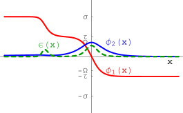
Figure 14: $K_{2}^{AB}(\gamma_{1})$ kinks: Profiles and energy density (left) Orbits in ${\mathbb{R}}^{2}$ (center) in ${\mathbb{E}}^{2}$ (right).

Again, it is easy to check that these singular kink combinations arise at the boundary of the $K_{2}^{AB}$ kink moduli space:

$$\lim_{\gamma_{1}\rightarrow\pm\infty}{K}_{2}^{AB}(\gamma_{1})\equiv\left\{\begin{array}[]{l}{K}_{1}^{AA}+{K}_{1}^{AB}\\ {K}_{1}^{BB}+{K}_{1}^{AB}\end{array}\right.\qquad.$$

In sum, there are six different types of kink solutions: four single kinks, the ${K}_{1}^{BF\bigvee FF\bigvee FB}$, the ${K}_{1}^{AB}$, the ${K}_{1}^{AA}$ and the ${K}_{1}^{BB}$ kinks, and two kink families, the ${K}_{2}^{BB}(\gamma_{1})$ and ${K}_{2}^{AB}(\gamma_{1})$ kink moduli spaces. The boundary of the ${K}_{2}^{BB}(\gamma_{1})$ family is a non-linear combination of the single kinks ${K}_{1}^{BF\bigvee FF\bigvee FB}$ and ${K}_{1}^{BB}$ whereas the boundary of the ${K}_{2}^{AB}(\gamma_{1})$ family is a non-linear combination of two single kinks: either ${K}_{1}^{BB}$ and ${K}_{1}^{AB}$ or ${K}_{1}^{AA}$ and ${K}_{1}^{AB}$.

4.3 Kink Variety in Regime II

Singular kinks

On the $\phi_{1}$ axis we again find the solutions (69) within the appropriate range of parameters.

1(a). ${K}_{2}^{A_{\pm}B_{\pm}}$: When $\sigma<|\phi(x)|<\tau$, the kink orbits connect the $A$ with the $B$ points and viceversa. The energy of these kinks is:

$${E}[{K}_{2}^{AB}]=\left|W(\pm\sigma,0)-W(\pm\tau,0)\right|=\frac{2\sqrt{2}}{15}\,(\sigma+\tau)^{3}(3\Omega-\sigma^{2}-\tau^{2})\qquad.$$

From the arguments of Section §3 one can identify these solitary waves as composite kinks formed by two basic kinks. One subtle point is the following: the kink orbits pass through one of the foci. Nevertheless, on the $\phi_{1}$ axis the foci are regular points of the superpotential. Although a pencil of kink orbits meet at the foci, the ${K}_{2}^{AB}$ trajectories do not belong to this congruence. We conclude that these composite kinks are stable.

1(b). ${K}_{1}^{B_{\pm}B_{\mp}}$: If $\sigma<|\phi_{1}(x)|$ (69), provides another type of solitary waves. The kink orbits are also located on the $\phi_{1}$ axis but link the $B_{+}$ and $B_{-}$ points and viceversa, see Figure 11. Their energy is:

$${E}[{K}_{1}^{B_{\pm}B_{\mp}}]=\left|W(\sigma,0)-W(-\sigma,0)\right|=\frac{4\sqrt{2}}{15}\,\sigma^{3}(5\tau^{2}-\sigma^{2})\qquad.$$

These kink orbits do not cross the foci and are thus stable.

On the ellipse (67) (left) two types of kinks live, ruled by the formula (70).

2(a). ${K}_{1}^{AC}$: If $1<|\phi_{1}(x)|<\tau$ and $\phi_{2}(x)=\pm\bar{\sigma}\sqrt{\tau^{2}-\phi_{1}^{2}(x)}$ the kink orbits connect the $A_{+}$ and the $C^{+}_{\pm}$ points (and also the $A_{-}$ and the $C^{-}_{\pm}$), see Figure 11. The energy of these kinks is:

$${E}[{K}_{1}^{AC}] = \left|W(\tau,0)-W(1,\pm\bar{\Omega})\right|=\left|W(-\tau,0)-W(-1,\pm\bar{\Omega})\right|$$

$$= \displaystyle\frac{\sqrt{2}}{15}\,\sigma^{3}(\tau-1)^{2}(2\sigma^{2}+4\sigma\Omega-10\tau^{2}+6\Omega^{2}-5\tau^{3}+3\Omega^{2}\tau)\qquad.$$

The kink orbits do not pass through the foci and these kinks are stable.

2(b). ${K}_{1}^{C^{-}C^{+}}$: If $1<|\phi_{1}(x)|$, formula (70) provides the other type of kinks with orbits in the quadric curve (67)(left). These kink orbits connect the points $C^{-}_{\pm}$ with $C^{+}_{\pm}$, see Figure 11. The kink energy is: ${E}[{K}_{1}^{C^{-}C^{+}}]=\left|W(-1,\pm\bar{\Omega})-W(1,\pm\bar{\Omega})\right|=\frac{4\sqrt{2}}{15}\,\sigma^{3}(5\tau^{2}-\sigma^{2})$ and these kinks are also stable. In this regime the quadric (67)(right) is a hyperbola:

$$\phi_{1}^{2}-\frac{\phi_{2}^{2}}{\tau^{2}-1}=\sigma^{2}\qquad.$$ (74)

3. ${K}_{1}^{C^{\pm}B_{\pm}}$: When $1>|\phi_{1}(x)|>\sigma$ and $\phi_{2}(x)=\pm|\bar{\tau}|\sqrt{\phi_{1}^{2}(x)-\sigma^{2}}$, formula (71) gives these kinks. The kink orbits connect $C^{-}_{\pm}$ with $B_{-}$ and $C^{+}_{\pm}$ with $B_{+}$, see Figure 11. The energy of these stable kinks is: $E[{K}_{1}^{CB}]=\left|W(-1,\pm\bar{\Omega})-W(-\sigma,0)\right|=\left|W(1,\pm\bar{\Omega})-W(\sigma,0)\right|=E[{K}_{2}^{AB}]-E[{K}_{1}^{AC}]$.

Generic kinks

In this regime of the model, the kink orbit and the kink profile general equations (38) and (39) provided by the Hamilton-Jacobi method become respectively:

$$\begin{array}[]{l}{\displaystyle\left\{\left(\frac{u-\sigma}{u+\sigma}\right)^{\frac{\tau^{3}}{\bar{\tau}^{2}(\tau^{2}-\sigma^{2})}}\left(\frac{u+\Omega}{u-\Omega}\right)^{\frac{1}{\bar{\sigma}^{2}\bar{\tau}^{2}}}\left(\frac{\tau-u}{\tau+u}\right)^{\frac{\sigma^{3}}{\bar{\sigma}^{2}(\tau^{2}-\sigma^{2})}}\right\}^{{\rm Sign}({u}^{\prime})}}\times\\[5.69046pt] \cdot\hskip 5.69046pt{\displaystyle\left\{\left|\frac{v+\sigma}{v-\sigma}\right|^{\frac{\tau^{3}}{\bar{\tau}^{2}(\tau^{2}-\sigma^{2})}}\left(\frac{\Omega-v}{\Omega+v}\right)^{\frac{1}{\bar{\sigma}^{2}\bar{\tau}^{2}}}\left(\frac{\tau+v}{\tau-v}\right)^{\frac{\sigma^{3}}{\bar{\sigma}^{2}(\tau^{2}-\sigma^{2})}}\right\}^{{\rm Sign}({v}^{\prime})}=e^{2\sqrt{2}\Omega^{3}\gamma_{1}}}\end{array}\quad,$$ (75)

$$\begin{array}[]{l}{\displaystyle\left\{\left(\frac{u-\sigma}{u+\sigma}\right)^{\frac{\tau}{\bar{\tau}^{2}(\tau^{2}-\sigma^{2})}}\left(\frac{u+\Omega}{u-\Omega}\right)^{\frac{1}{\bar{\sigma}^{2}\bar{\tau}^{2}}}\left(\frac{\tau-u}{\tau+u}\right)^{\frac{\sigma}{\bar{\sigma}^{2}(\tau^{2}-\sigma^{2})}}\right\}^{{\rm Sign}({u}^{\prime})}}\times\\[5.69046pt] \cdot\hskip 5.69046pt{\displaystyle\left\{\left|\frac{v-\sigma}{v+\sigma}\right|^{\frac{\tau}{\bar{\tau}^{2}(\tau^{2}-\sigma^{2})}}\left(\frac{\Omega+v}{\Omega-v}\right)^{\frac{1}{\bar{\sigma}^{2}\bar{\tau}^{2}}}\left(\frac{\tau-v}{\tau+v}\right)^{\frac{\sigma}{\bar{\sigma}^{2}(\tau^{2}-\sigma^{2})}}\right\}^{{\rm Sign}({v}^{\prime})}=e^{2\sqrt{2}\Omega(x+\gamma_{2})}}\end{array}\quad.$$ (76)

In ${\mathbb{R}}^{2}$, the boundaries of the cells are formed by pieces of the ellipse (67) (left), the hyperbola (74), and the $\phi_{1}$ axis, see Figure 15. Although there are three cells in this regime, two of them are related by the symmetries of the model. The analysis is thus restricted to the $C_{-11}^{23}$ and $C_{12}^{23}$ cells. From the curves determined by (75) and (76), we find the following three types of kink families:

4(a). ${K}_{2}^{B_{\pm}C^{+}_{\mp}}(\gamma_{1})$: In the cell $C_{-11}^{23}$ the trajectories determined by (75) and (76) connect the points $B_{+}$ with $C^{+}_{-}$ -skipping the saddle points $B_{-}$ and $C^{+}_{+}$- or $B_{-}$ with $C^{+}_{+}$ -skipping the saddle points $B_{+}$ and $C^{+}_{-}$-, depending on the sign of the combinations ${\rm Sign}({u}^{\prime})={\rm Sign}({v}^{\prime})$ and ${\rm Sign}({u}^{\prime})\neq{\rm Sign}({v}^{\prime})$. The orbits of these ${K}_{2}^{B_{\pm}C^{+}_{\mp}}(\gamma_{1})$ one-parametric kink families do not cross the foci, see Figure 15, and the kinks are stable.

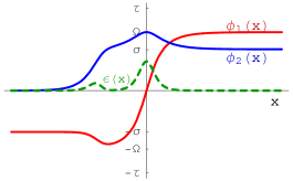
Figure 15: ${K}_{2}^{B_{\pm}C^{+}_{\mp}}(\gamma_{1})$ kinks: Profiles and energy density (left) Orbits in ${\mathbb{R}}^{2}$ (center) in ${\mathbb{E}}^{2}$ (right).

The energy of any member of these families of topological kinks and the kink mass sum rules are:

$${E}[{K}_{2}^{B_{\pm}C^{+}_{\mp}}(\gamma_{1})] = \left|W(\pm\sigma,0)-W(1,\mp\bar{\Omega})\right|=E[{K}_{1}^{B_{\pm}C^{+}_{\pm}}]+E[{K}_{1}^{C_{\mp}^{+}C^{+}_{\pm}}]=E[{K}_{1}^{B_{\pm}C^{+}_{\pm}}]+E[{K}_{1}^{B_{\mp}B_{\pm}}]$$

$$= \frac{\sqrt{2}}{15}(-4\sigma^{5}+20\sigma\Omega^{2}+10\Omega^{2}\tau+15\Omega^{3}-5\sigma^{2}\Omega^{3}-2\tau^{5}-5\Omega^{3}\tau^{2}+3\Omega^{5})\qquad.$$

This result perfectly fits the infinite $\gamma_{1}$ limit of the family:

$$\lim_{\gamma_{1}\rightarrow\pm\infty}{K}_{2}^{B_{\pm}C^{+}_{\mp}}(\gamma_{1})\equiv\left\{\begin{array}[]{l}{K}_{1}^{B_{\pm}C^{+}_{\pm}}+{K}_{1}^{C^{+}_{\mp}C^{+}_{\pm}}\\ {K}_{1}^{B_{\pm}C^{+}_{\pm}}+{K}_{1}^{B_{\mp}B_{\pm}}\end{array}\right.\qquad\qquad.$$

4.(b) ${K}_{2}^{A_{+}B_{+}}(\gamma_{1})$ and ${K}_{2}^{A_{-}B_{-}}(\gamma_{1})$: Inside the cells $C_{12}^{23}$ and $C_{-2-1}^{23}$, the trajectories determined by the equations (75) and (76) for any sign combination respectively connect the $A_{+}$ ($A_{-}$) and $B_{+}$ ($B_{-}$) nodal points without crossing any focal point, see Figure 16. These heteroclinic orbits thus provide a family of stable topological kinks (one family per cell).

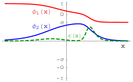
Figure 16: ${K}_{2}^{BC}(\gamma_{1})$ kinks: Profiles and energy density (left) Orbits in the Cartesian plane (center) and elliptic plane (right).

The energy of these topological kinks is:

$${E}[{K}_{2}^{A_{\pm}B_{\pm}}(\gamma_{1})]=\left|W(\pm\tau,0)-W(\pm\sigma,0)\right|=\frac{2\sqrt{2}}{15}(\sigma+\tau)^{3}(3\Omega-\sigma^{2}-\tau^{2})\qquad.$$

The kink mass sum rule

$$E[{K}_{2}^{A_{\pm}B_{\pm}}(\gamma_{1})]=E[{K}_{1}^{AC}]+E[{K}_{1}^{CB}]=E[{K}_{2}^{AB}]$$

means that the infinite $\gamma_{1}$ limit of the family is:

$$\lim_{\gamma_{1}\rightarrow\pm\infty}{K}_{2}^{A_{\pm}B_{\pm}}(\gamma_{1})\equiv\left\{\begin{array}[]{l}{K}_{1}^{AC}+{K}_{1}^{CB}\\ {K}_{2}^{BC}\end{array}\right.\qquad\qquad.$$

5. ${K}_{4}^{C^{+}_{-}F_{-}\bigvee F_{-}C^{-}_{-}}(\gamma_{1})$ and ${K}_{4}^{C^{+}_{+}F_{+}\bigvee F_{+}C^{-}_{+}}(\gamma_{1})$: In the $C_{12}^{23}$ and $C_{-2-1}^{23}$ cells equations (75) and (76) include trajectories passing from one $C^{+}$ point to a focus and from a focus to a $C^{-}$ point ( or viceversa) for any combination of signs. Kink orbits (homoclinic in ${\mathbb{E}}^{2}$, heteroclinic in ${\mathbb{R}}^{2}$) are formed by continuously gluing at a focus two of these trajectories, one with ${\rm Sign}(u)^{\prime}={\rm Sign}(v)^{\prime}$ and the other with ${\rm Sign}(u)^{\prime}\neq{\rm Sign}(v)^{\prime}$. In this way, two families of topological kinks are obtained with orbits starting from one of the $C^{+}_{\pm}$ points, crossing the $F_{\pm}$ focus, and ending at the correlative point $C^{-}_{\pm}$, see Figure 17. The energy of these unstable topological kinks is:

$${E}[{K}_{4}^{C^{+}F\bigvee FC^{-}}(\gamma_{1})] = \left|W(1,\pm\bar{\Omega})-W(\pm\Omega,0)\right|+\left|W(\pm\Omega,0)-W(-1,\pm\bar{\Omega})\right|$$

$$= \frac{4\sqrt{2}}{15}(\sigma+\tau)^{3}(3\Omega-\tau^{2}-\sigma^{2})$$

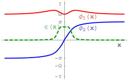
Figure 17: ${K}_{4}^{C^{+}_{+}C^{-}_{+}}(\gamma_{1})$ kinks: Profiles and energy density (left) Orbits in ${\mathbb{R}}^{2}$ (center) in ${\mathbb{E}}^{2}$ (right).

The kink mass sum rule is ${E}[{K}_{4}^{C^{+}F\bigvee FC^{-}}(\gamma_{1})]={E}[{K}_{1}^{CB}]+{E}[{K}_{2}^{AB}(\gamma_{1})]+{E}[{K}_{1}^{AC}]$ in agreement with the $\gamma_{1}\rightarrow\infty$ limit of the family:

$$\lim_{\gamma_{1}\rightarrow\pm\infty}{K}_{4}^{C^{+}F\bigvee FC^{-}}(\gamma_{1})\equiv{K}_{1}^{CB}+{K}_{2}^{AB}(\gamma_{1})+{K}_{1}^{Ac}\qquad.$$

In sum, the kink variety in this regime is formed by seven kinds of solitary waves. (1) Four singles kinks: ${K}_{1}^{AC}$, ${K}_{1}^{CB}$, ${K}_{1}^{BB}$ and ${K}_{1}^{CC}$. (2) Three kink families: ${K}_{2}^{BC}(\gamma_{1})$, ${K}_{2}^{AB}(\gamma_{1})$ and ${K}_{4}^{CC}(\gamma_{1})$. Members of the ${K}_{2}^{BC}(\gamma_{1})$ family are composite kinks formed by a pair of either ${K}_{1}^{CC}$-${K}_{1}^{CB}$ or ${K}_{1}^{BC}$-${K}_{1}^{BB}$ kinks. The basic kink inter-center distance in each pair is finite and is determined by the $\gamma_{1}$ parameter. Basic kinks appear liberated from each other (infinite inter-center distance) when $|\gamma_{1}|=\infty$. The kinks of the ${K}_{2}^{AB}(\gamma_{1})$ family are similar non-linear combinations of two single kinks: the ${K}_{1}^{AC}$-${K}_{1}^{CB}$ kink pair arise at the $\gamma_{1}=\infty$ boundary of the ${K}_{2}^{AB}(\gamma_{1})$ moduli space. There is, however, a subtle point: at the $\gamma_{1}=-\infty$ boundary lives the ${K}_{2}^{AB}$ kink, which is thus a composite but singular kink. Finally, the structure of the ${K}_{4}^{CF\bigvee FC}(\gamma_{1})$ kinks is even more complex. These kinks can be thought of as non-linear combinations of the ${K}_{1}^{AC}$, ${K}_{2}^{BA}$ and ${K}_{1}^{BC}$ basic kinks when the distances between the three centers are finite.

4.4 Kink Variety in Regime III

Singular kinks

In this regime the ansatz $\phi_{2}=0$ plugged into (69) gives rise to two types of kink orbits.

1(a). ${K}_{1}^{A_{\pm}B_{\pm}}$: These orbits connect the points $A_{+}$ with $B_{+}$ or $A_{-}$ with $B_{-}$, see Figure 12. The energy of the corresponding kinks is: ${E}[{K}_{1}^{AB}]=\left|W(\pm 1,0)-W(\pm\Omega,0)\right|=\frac{2\sqrt{2}}{15}(1-\Omega)^{3}(1+\Omega(3+\Omega))$.

1(b). ${K}_{1}^{B_{+}B_{-}}$: There is also a kink orbit on the $\phi_{1}$-axis connecting $B_{+}$ with $B_{-}$. The kink energy is: ${E}[{K}_{1}^{B_{+}B_{-}}]=\left|W(\Omega,0)-W(-\Omega,0)\right|=\frac{4\sqrt{2}}{15}\Omega^{3}(5-\Omega^{2})$.

The third type of singular kink in regime III lives on the ellipse (67)(left).

2. ${K}_{1}^{A_{+}A_{-}}$: These elliptic kink orbits are given by (70 and) connect the $A_{+}$ and $A_{-}$ points, see Figure 12. The kink energy is: ${E}[{K}_{1}^{A_{+}A_{-}}]=\left|W(1,0)-W(-1,0)\right|=\frac{4\sqrt{2}}{15}\Omega^{3}(5-\Omega^{2})={E}[{K}_{1}^{B_{+}B_{-}}]$.

Generic kinks

The Hamilton-Jacobi procedure provides the kink orbits

$$\begin{array}[]{l}{\displaystyle\left\{\left(\frac{u+\sigma}{u-\sigma}\right)^{\frac{1-3\sigma^{2}}{2}}\left(\frac{1+u}{1-u}\right)^{\sigma^{3}}{\rm exp}\left[{\frac{-\sigma\bar{\sigma}^{2}u}{u^{2}-\sigma^{2}}}\right]\right\}^{{\rm Sign}({u}^{\prime})}\times}\\ {\displaystyle\left\{\left(\frac{\sigma-v}{\sigma+v}\right)^{\frac{1-3\sigma^{2}}{2}}\left(\frac{1-v}{1+v}\right)^{\sigma^{3}}{\rm exp}\left[{\frac{\sigma\bar{\sigma}^{2}v}{v^{2}-\sigma^{2}}}\right]\right\}^{{\rm Sign}({v}^{\prime})}=e^{2\sqrt{2}\sigma^{3}\gamma_{1}}}\end{array}\qquad,$$ (77)

and the kink profiles

$$\begin{array}[]{l}{\displaystyle\left\{\left(\frac{u-\sigma}{u+\sigma}\right)^{\frac{1-3\sigma^{2}}{2\sigma^{3}}}\left(\frac{1-u}{1+u}\right){\rm exp}\left[{\frac{\bar{\sigma}^{2}u}{\sigma^{2}(u^{2}-\sigma^{2})}}\right]\right\}^{{\rm Sign}({u}^{\prime})}\times}\\ {\displaystyle\left\{\left(\frac{\sigma+v}{\sigma-v}\right)^{\frac{1-3\sigma^{2}}{2\sigma^{3}}}\left(\frac{1+v}{1-v}\right){\rm exp}\left[{\frac{-\bar{\sigma}^{2}v}{\sigma^{2}(v^{2}-\sigma^{2})}}\right]\right\}^{{\rm Sign}({v}^{\prime})}=e^{2\sqrt{2}(x+\gamma_{2})}}\end{array}$$ (78)

of Regime III in the $C_{-11}^{12}$ cell.

3. ${K}_{2}^{A_{-}B_{+}}(\gamma_{1})$ and ${K}_{2}^{A_{+}B_{-}}(\gamma_{1})$: Equations (77) and (78) describe two families of topological kinks joining the $A_{\pm}$ with the $B_{\mp}$ points, see Figure 16..

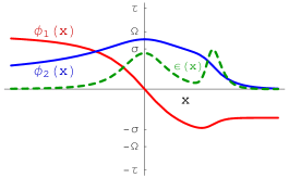
Figure 18: ${K}_{2}^{A_{-}B_{+}}(\gamma_{1})$ kinks: Profiles and energy density (left) Orbits in ${\mathbb{R}}^{2}$ (center) in ${\mathbb{E}}^{2}$ (right).

The kink energy is:

$${E}[{K}_{2}^{A_{\pm}B_{\mp}}(\gamma_{1})]=\left|W(\pm 1,0)-W(\mp\Omega,0)\right|=\frac{2\sqrt{2}}{15}(1-5\Omega^{2}+15\Omega^{3}-3\Omega^{5})\qquad,$$

such that the kink mass sum rules hold:

$${E}[{K}_{2}^{A_{\pm}B_{\mp}}(\gamma_{1})]=E[{K}_{1}^{A_{-}A_{+}}]+E[{K}_{1}^{A_{+}B_{+}}]=E[{K}_{1}^{B_{-}B_{+}}]+E[{K}_{1}^{A_{-}B_{-}}]\qquad\qquad,$$

in agreement with the $|\gamma_{1}|=\infty$ limit of the family

$$\lim_{\gamma_{1}\rightarrow\pm\infty}{K}_{2}^{A_{\pm}B_{\mp}}(\gamma_{1})\equiv\left\{\begin{array}[]{l}{K}_{1}^{A_{-}A_{+}}+{K}_{1}^{A_{+}B_{+}}\\ {K}_{1}^{B_{-}B_{+}}+{K}_{1}^{A_{-}B_{-}}\end{array}\right.\qquad\qquad.$$

4.5 Kink mass sum rules

A summary of the different kink mass sum rules is as follows:

- Kink mass sum rules in regime I:
$E[K_{1}^{AA}]=E[K_{1}^{BB}]$
$E[K_{2}^{AB}(\gamma_{1})]=E[K_{1}^{AB}]+E[K_{1}^{BB}]$
$E[K_{2}^{BB}(\gamma_{1})]=E[{K}_{1}^{BF\bigvee FF\bigvee FB}]+E[K_{1}^{BB}]$

- Kink mass sum rules in regime II:
$E[K_{1}^{BB}]=E[K_{1}^{C^{+}C^{+}}]$
$E[K_{2}^{B_{\mp}C_{\pm}^{+}}(\gamma_{1})]=E[K_{1}^{BC^{+}}]+E[K_{1}^{C^{+}_{\mp}C^{+}_{\pm}}]$
$E[K_{2}^{AB}]=E[{K}_{1}^{AC^{+}}]+E[K_{1}^{C^{+}B}]$
$E[K_{2}^{AB}(\gamma_{1})]=E[K_{2}^{AB}]$
$E[K_{4}^{C^{+}F\bigvee FC^{+}}(\gamma_{1})]=2E[K_{2}^{AB}(\gamma_{1})]$

- Kink mass sum rules in regime III:
$E[K_{1}^{AA}]=E[K_{1}^{BB}]$
$E[K_{2}^{AB}(\gamma_{1})]=E[K_{1}^{AB}]+E[K_{1}^{BB}]$

5 Summary and Outlook

The developments discussed in this paper unveil the structure of a broad class of two-component scalar field theory models, which generalize the well-studied MSTB model. It is well known that the search for static solutions in (1+1)D scalar field theory is tantamount to the solving of an analogous mechanical system with flipped potential with respect to the field theoretical model. The generalized MSTB models are characterized by: (1) Having a Type I Liouville analogous mechanical system. These mechanical systems are Hamilton-Jacobi separable by using elliptic coordinates. (2) Having a discrete set of unstable critical points of the mechanical potential, homogeneous solutions or “vacua” in the field theory. This feature supports the existence of very rich varieties of heteroclinic and homoclinic separatrix trajectories in the mechanical problem, and topological and non-topological solitary waves or kinks in the field theory setting.

We have shown the following structural properties:

• The “vacua” of the field theoretical system and the foci of the elliptic and hyperbolic coordinating curves are placed at the junctions of a rectangular mesh displayed on the elliptic strip, which is divided into different cells where the dynamics runs separately.

• The distribution of the vacua on this reticulum depends on the details of the potential energy density of the model.

• There exist only three types of cells in the mesh. In Type I cells, the vacua of the model sit on the four vertices. Only three vertices are vacua in Type II cells, whereas one of the two foci sits at the fourth vertex. Finally, in Type III cells two vacua and two foci occupy the four vertices.

• The cell of the reticulum is the cornerstone that determines the structure of the kink variety. There exist two families of kink solutions confined in each cell and single kinks living on the edges of the cell. The characteristics of these kinks, in particular their stability, do not depend on the details of the potential density but only on the type of the cell in which they are confined.

• The different kink families are described thoroughly. Because the separability of the mechanical model, kink mass sum rules arise between at least two types of kinks.

• For this reason, each member of a kink family (confined inside the cell) is indeed a composite kink that can be understood as a non-linear combination of several single kinks (settled at the edges of the cell).

• In sum, the potential energy density of the field theoretical model determines the reticulum bounding the cells and the cells determine the behavior and structure of the kink families. Therefore, a qualitative description of the kink variety of generalized MSTB models is do-able by merely observing the expression of the potential energy density in elliptic coordinates.

We finish by noticing that the scheme developed in this paper can be extended to other two-component scalar field theoretical models. In particular, models with Type III and II Liouville analogous mechanical systems, respectively Hamilton-Jacobi separable using parabolic and polar coordinates, have very similar structures. We believe, however, that the Type I models are primordial because parabolic and polar coordinates are special limits of the system of elliptic coordinates.

6 Acknowledgements

We are very grateful to Hernan Augusto Piragua Ariza for reporting us some typos in the introduction included in the first version of the manuscript.

References

- [1]
- [2] H. Ito, H. Tasaki, Stability theory for non-linear Klein-Gordon kinks and Morse’s index theorems, Phys. Lett. A113 (1985) 179-182.
- [3] A.H. Eschenfelder, Magnetic Bubble Technology, (1981) Berlin, Springer-Verlag.
- [4] F. Jona and G. Shirane, Ferroelectric Crystals, (1993) New York, Dover; E.K. Salje, Phase Transitions in Ferroelastic and Co-Elastic Crystals, Cambridge, UK, Cambridge University Press; B.A. Strukov and A. Levanyuk, Ferroelectric Phenomena in Crystals, Berlin, Springer-Verlag.
- [5] J.M. Harris, Poly(ethylene glycol) chemistry: Biotechnical and Biomedical Applications, (1992) New York, Plenum.
- [6] A. S. Davydov, Solitons in molecular systems, (1985) Dordrech, D. Reidel.
- [7] R. Rajaraman, Solitons and Instantons, (1982) North-Holland, Amsterdam.
- [8] M.K. Prasad, C.M. Sommerfield, Phys. Rev. Lett 35 (1975) 760; E.B. Bogomol’nyi, Sov. J. Nucl. Phys. 24 (1976) 449.
- [9] D. Bazeia, H. Boschi-Filho, F.A. Brito, Domain Defects in systems of two real scalar fields, J. High Energy Phys. 4 (1999) 28.
- [10] D. Bazeia, M.J. Dos Santos, R.F. Ribeiro, Solitons in systems of coupled scalar fields, Phys. Lett. A208 (1995) no. 1-2, 84-88.
- [11] D. Bazeia, J.R.S. Nascimento, R.F. Ribeiro, D. Toledo, Soliton stability in systems of two real scalar fields, J. Phys. A30 (1997) no. 23, 8157-8166.
- [12] F.A. Brito, D. Bazeia, Domain ribbons inside domain walls at finite temperature, Phys. Rev. D56 (1997) no. 12, 7869-7876.
- [13] J.D. Edelstein, M.L. Trobo, F.A. Brito, D. Bazeia, Kinks inside supersymmetric domain ribbons, Phys. Rev. D57 (1998) no. 12, 7561-7569.
- [14] D. Bazeia, J. Menezes, R. Menezes, Mod. Phys. Lett. B19 (2005) 801-819.
- [15] J.R. Morris, Nested domain defects, Int. J. Mod. Phys. A13 (1998) 1115-1128.
- [16] P. Sutcliffe, Domain wall networks on solitons, Phys. Rev. D68 (2003) 085004.
- [17] D. Bazeia, L. Losano, C. Wotzasek, Domain walls in three-field model, Phys. Rev. D62 (2000) 101701.
- [18] C. Montonen, On solitons with an abelian charge in scalar field theories (I) Classical theory and Bohr-Sommerfeld quantization, Nucl. Phys. B112 (1976) 349.
- [19] S. Sarker, S.E. Trullinger, A.R. Bishop, Solitay-wave solution for a complex one-dimensional field, Phys. Lett. 59A (1976) 255-258.
- [20] Rajaraman, R. y Weinberg, E.J., Phys. Rev. D11 (1975) 2950.
- [21] J. F. Currie, S. Sarker, A. R. Bishop and S. E. Trullinger, Phys. Rev. A20 (1979) 2213.
- [22] S. E. Trullinger and R. M. deLeonardis, Phys. Rev. B 22 (1980) 5522.
- [23] R. Rajaraman, Phys. Rev. Lett. 42 (1979) 200-204.
- [24] K.R. Subbaswamy, S.E. Trullinger, Instability of non topological solitons of coupled scalar field theories in two dimensions, Phys. Rev. D22 (1980) 1495-1496.
- [25] K.R. Subbaswamy, S.E. Trullinger, Intriguing properties of kinks in a simple model with a two-component field, Physica2D (1981) no. 2, 379-388.
- [26] E. Magyari, H. Thomas, Solitary waves in a 1D anharmonic lattice with two-component order parameter, Phys. Lett. 100A (1984) no. 1, 11-14.
- [27] R. Garnier, Sur une class de systemes differentielles Abeliens deduits del theorie des equations lineaires, Rend. Circ. Mat. Palermo 43 (1919) 155-191.
- [28] H. Ito, Kink energy sum rule in a two-component scalar field model of 1+1 dimensions, Phys. Lett. 112A (1985) 119-123.
- [29] J. Mateos Guilarte, J., A note on Morse theory and one-dimensional solitons, Lett. Math. Phys., 14 (1987) 169-176.
- [30] J. Mateos Guilarte, Stationary phase approximation and quantum soliton families, Annals of Physics, 188 (1988) 307-346.
- [31] A. Alonso-Izquierdo, M.A. González León, W. García Fuertes, J. Mateos Guilarte, Semi-classical mass of quantum k-component topological kinks, Nucl. Phys. B638 (2002) 378-404.
- [32] J. Mateos Guilarte, Sphalerons and instantons in two-dimensional field theory, Annals of Physics, 216 (1992) 122-151.
- [33] A. Alonso-Izquierdo, M.A. González León, J. Mateos Guilarte, Kink manifolds in (1+1)-dimensional scalar field theory, J. Phys. A: Math. Gen. 31 (1998), 209-229.
- [34] A. Alonso-Izquierdo, M.A. Gonzalez Leon, J. Mateos Guilarte and M. de la Torre Mayado, Kink variety in systems of two coupled scalar fields in two space-time dimensions, Phys. Rev. D 65 (2002) 085012.
- [35] A. Alonso-Izquierdo, J. Mateos Guilarte, One-dimensional solitary waves in singular deformations of SO(2) invariant two-component scalar field theory models, Nonlinearity 20 (2007) 2691-2719.
- [36] A. Alonso-Izquierdo, M.A. Gonzalez Leon, J. Mateos Guilarte and M. de la Torre Mayado, Adiabatic motion of two-component BPS kinks, Phys. Rev. D 66 (2002) 105022.
- [37] A. Alonso-Izquierdo, M.A. Gonzalez Leon, M. de la Torre Mayado, J. Mateos Guilarte, Changing shapes: adiabatic dynamics of composite solitary waves, Physica D 200 (2005) 220-241.
- [38] A. Alonso-Izquierdo, M. A. Gonzalez Leon, and J. Mateos Guilarte, Kink from dynamical systems: domain walls in a deformed linear sigma model, Nonlinearity 13 (2000), 1137-1169.
- [39] A. Alonso-Izquierdo, M. A. Gonzalez Leon, and J. Mateos Guilarte, Stability of kink defects in a deformed linear sigma model, Nonlinearity 15 (2002), 1097-1125.
- [40] A. Alonso-Izquierdo, J.C. Bueno Sánchez, M. A. Gonzalez Leon, and M. de la Torre Mayado, Kink manifolds in a three-component scalar field theory, J. Phys. A: Math. Gen. 37 (2004), 3607-3626.
- [41] A. Alonso-Izquierdo, and J. Mateos-Guilarte, Composite solitary waves in three-component scalar field theory: three-body low energy scattering, Physica D200 (2006) 31-53.
- [42] A. Perelomov, Integrable Systems of Classical Mechanics and Lie Algebras, (1990) Birkhäuser, Boston MA.